Suzaku Observations of Three FeLoBAL QSOs, SDSS J0943+5417, J1352+4239, and J1723+5553

Abstract

We present Suzaku observations of three iron low-ionization broad absorption line quasars (FeLoBALs). We detect J1723+5553 ($3\sigma$) in the observed 2–10 keV band, and constrain its intrinsic ${N}_{\rm H}$ column density to $\hbox{${N}_{\rm H}$}>6\times 10^{23}$ cm^-2 by modeling its X-ray hardness ratio. We study the broadband spectral index, $\alpha_{\rm ox}$, between the X-ray and UV bands by combining the X-ray measurements and the UV flux extrapolated from 2MASS magnitudes, assuming a range of intrinsic column densities, and then comparing the $\alpha_{\rm ox}$ values for the three FeLoBALs with those from a large sample of normal quasars. We find that the FeLoBALs are consistent with the spectral energy distribution (SED) of normal quasars if the intrinsic ${N}_{\rm H}$ column densities are $\hbox{${N}_{\rm H}$}>7\times 10^{23}$ cm^-2 for J0943+5417, $\hbox{${N}_{\rm H}$}>2\times 10^{24}$ cm^-2 for J1352+4293, and $6\times 10^{23}<\hbox{${N}_{\rm H}$}<3\times 10^{24}$ cm^-2 for J1723+5553. At these large intrinsic column densities, the optical depth from Thomson scattering can reach $\sim 6$, which will significantly modulate the UV flux. Our results suggest that the X-ray absorbing material could be located at a different place from the UV absorbing wind, likely between the X-ray and UV emitting regions. We find a significant kinetic feedback efficiency for FeLoBALs, indicating that the outflows are an important feedback mechanism in quasars.

1 Introduction

Quasars and active galactic nuclei (AGN) are ubiquitous phenomena wherever we look in the universe. The subset of quasars known as broad absorption line quasars (BALQSOs) are characterized by blue-shifted, rest-frame UV absorption troughs due to gas outflow. Even before the first definitive survey in Weymann et al. (1991), BALQSOs provided a unique glimpse into the central engines of AGN, where the nature of the intrinsic absorption has important implications for the structure of the central engine. To classify a quasar as a BALQSO, the traditional definition of Weymann et al. (1991) requires the absorption troughs to be at least 2,000 km s^-1 wide. Recent studies have relaxed this, e.g., Trump et al. (2006), to include quasars with absorption troughs over 1,000 km s^-1 in width. Regardless of which definition is used, BALQSOs are further divided into those that exhibit absorption troughs from only high-ionization species (HiBALs) and those with low-ionization species (LoBALs). Most BALQSOs are HiBALs, and most LoBALs also have high-ionization troughs in their spectra (Weymann et al., 1991; Trump et al., 2006). LoBALs are further classified by the low-ionization species they exhibit: in this paper, the objects surveyed have strong iron absorption, and are therefore iron LoBALs (FeLoBALs). This type of BALQSO is rare, and comprises only 1.5–2.1% of the entire quasar population (Dai et al., 2010b), while LoBALs and BALQSOs make up $\sim$4–7% (Dai et al., 2010b) and $\sim$20–40% (Dai et al., 2008; Shankar et al., 2008a; Ganguly & Brotherton, 2008; Knigge et al., 2008; Maddox et al., 2008; Allen et al., 2010), respectively, depending on the threshold of the trough width. Focusing on FeLoBALs is meaningful because of their unique characteristics and the bearing they have on the broader picture: either as an evolutionary link in the normal AGN lifetime, or as a geometric interpretation of a uniform class of objects.

Besides the low-ionization absorption lines, the optical continua for LoBALs are more reddened than HiBALs and normal QSOs, suggestive of stronger dust absorption, perhaps from large quantities of dust in the vicinity of the central engine (Sprayberry & Foltz, 1992). LoBALs in particular are more apparently X-ray weak than normal BALQSOs (Green et al., 2001; Gallagher et al., 2002a). There is a large portion, $\sim$80%, not detected in X-rays, along with lower than expected values for the UV to X-ray luminosity ratio, $\alpha_{\rm ox}$ ($\alpha_{\rm ox}$ lower than expected by $\sim-0.9$), that leads most previous studies, e.g. Green et al. (2001); Gallagher et al. (2002a), to conclude that there is extreme X-ray absorption in LoBALs. Streblyanska et al. (2010), however, found that LoBALs in general have lower column densities ($N_{H}<10^{22}$ cm^-2) than HiBALs. This conclusion may have been influenced by their X-ray bright sample, required for sufficient quality to perform X-ray spectral analyses.

Low-ionization BALQSOs with broad iron absorption lines (FeLoBALs) represent an extreme category. They have the reddest continuum spectra, complex UV spectra, and possibly largest X-ray absorption column densities. There are a handful of FeLoBALs already studied in X-rays, with only a few detections. Almost all were observed using the sensitive X-ray telescope, Chandra. The nearby FeLoBAL Mrk 231 ($z=0.042$) was also detected by XMM-Newton and BeppoSAX (Turner & Kraemer, 2003; Braito et al., 2004) in addition to Chandra (Gallagher et al., 2002b), which allowed for the most in-depth studies of an FeLoBAL to date. All three studies find the 0.4–10 keV X-ray emission to be mostly reflected and scattered into our line of sight, and the direct X-ray emission is mostly absorbed. Using the PDS detector on board BeppoSAX, Braito et al. (2004) detect the direct X-ray emission of Mrk 231 at $3\sigma$ in the 15–60 keV band, which allows the authors to constrain an intrinsic column density $N_{H}\sim 2\times 10^{24}$ cm^-2. Another recent study focused on two FeLoBALs is Rogerson et al. (2011), where the authors calculated $\alpha_{\rm ox}$ upper limits for both objects, comparing them with a large sample of normal AGN (Steffen et al., 2006). Other studies focused on subsets of quasars, but had FeLoBALs contained within their scope. Quite a few of these focused on radio-detected objects. In one study, Urrutia et al. (2005) selected 12 luminous red quasars, with the criteria that they were also detected by FIRST (Becker et al., 1995), and used standard aperture photometry (for details see § 2.2) to conduct X-ray analyses. They found that all of their objects are X-ray absorbed to some degree; in addition, they found a slightly steeper spectral slope than that for normal quasars, with an unweighted mean of $\Gamma=2.2\pm 0.4$ and a high-energy region weighted mean of $\Gamma=2.1\pm 0.5$. Brotherton et al. (2005) selected five radio-loud BALQSOs, three of which are LoBALs, and two of those LoBALs exhibited iron features. The three LoBALs were found to exhibit the steepest $\alpha_{\rm ox}$ values in the study. Miller et al. (2009) also selected 21 radio-loud BALQSOs, one of which is classified as an FeLoBAL. The authors proposed that the X-ray properties are explained by a model that consists of X-ray emission in the disk/corona and linked to the radio-jet. Almost all of these studies calculated intrinsic column density for these objects, most of which are in the 10²² – 10²⁴ cm^-2 range. These will be discussed in detail in § 5.2. In this study, we will use our X-ray detections and non-detections to constrain X-ray absorption column densities. One of our objects is the first X-ray detection (at the 3$\sigma$ level) by Suzaku of an FeLoBAL.

It is not understood why FeLoBALs possess unique physical characteristics; evolution and geometry are the contending theories. A geometric interpretation (e.g., Elvis, 2000) proposes that the broad absorption line region of a BALQSO simply arises from looking straight down a narrow outflow, while normal AGN and quasars are the same object viewed from different angles. A recent discovery of a LoBAL transitioning from an FeLoBAL within a few years rest frame favors special lines of sight, because of the short time scale (Hall et al., 2010). On the other hand, Lípari et al. (2009) proposed that BALQSOs, and FeLoBALs especially, are early progenitors of normal AGN and quasars, at the very end of an extreme starburst period and in the process of blowing out material from type II SNe that is Fe II rich. This evolutionary theory is partially supported by the higher fraction of LoBALs at high IR luminosities (e.g., Farrah et al., 2007; Urrutia et al., 2009; Dai et al., 2010b). A recent Spitzer spectral survey of six FeLoBALs (Farrah et al., 2010) showed significant signatures of dust and PAH emissions. Spectral modelings in the UV regime also support a large covering fraction of the wind for FeLoBALs (e.g., Casebeer et al., 2008). Other evidence, such as the decreasing fraction as a function of radio luminosity, is consistent with a geometric interpretation (Shankar et al., 2008a; Dai et al., 2010b). Therefore, the population of LoBALs and FeLoBALs could also be a combination of both evolution and geometry (Dai et al., 2010b).

Another interesting question is how FeLoBALs contribute to the quasar feedback process. AGN feedback is widely used in galaxy formation models (e.g., Granato et al. 2004; Scannapieco & Oh 2004; Hopkins et al. 2005; Shankar et al. 2008b) to explain the co-evolution of AGN and their host galaxies. Feedback can reproduce such phenomena as the $M$–$\sigma$ relation (e.g., Graham et al., 2011; Gültekin et al., 2009), star formation rates (Silk & Nusser, 2010), and even the shortfall in the halo baryon fraction (Silk & Nusser, 2010). Whether FeLoBALs are an evolutionary stage or a geometric interpretation of AGN, studying their feedback efficiency allows us to add to our limited picture of their physical characteristics.

In this paper we present new Suzaku observations of three FeLoBALs, SDSS objects J094317.59+541705.1, J135246.37+423923.5, and J172341.08+555340.5 (hereafter J0943+5417, J1352+4239, and J1723+5553, respectively). The targets are classified as FeLoBALs by Trump et al. (2006), and are the brightest ($K_{s}<$ 14.4 mag) of the 2 Micron All Sky Survey (2MASS) selected BALQSOs (Dai et al., 2008). J0943+5417 is a radio-intermediate quasar detected with a peak flux of 1.71 mJy/beam and RMS noise of 0.145 mJy/beam by Faint Images of the Radio Sky at Twenty-Centimeters (FIRST). None of these objects are detected at the flux limit in the NRAO/VLA Sky Survey (Condon et al., 1998). J0943+5317 and J1352+4239 are typical FeLoBALs with extremely complex rest frame UV spectra, whereas J0943+5417 has absorption troughs so wide that they overlap and completely suppress the UV continuum. We extrapolate our UV data from 2MASS, which samples the rest frame optical bands, and then correct to the rest frame UV. The complexity of the observed optical/rest frame UV spectra makes it extremely difficult to model the continuum. This is addressed in § 3. Since the targets all have redshifts $z\sim 2$, the XIS on-board Suzaku can probe the rest frame energy up to 30 keV, where the rest frame 6–30 keV (observed 2–10 keV) emission is only moderately affected by absorption even if $\hbox{${N}_{\rm H}$}\sim 10^{24}\hbox{cm${}^{-2}$}$, allowing us to detect the FeLoBALs if they are Compton thin. We study the relationship between X-ray and UV luminosities for these three FeLoBALs, and compare our values to a large sample of optically selected normal quasars. Our Suzaku observations and data reduction are described in §2, followed by calculations of 2500Å luminosities in §3. Section 4 presents results, followed by discussion in §5. Throughout the paper we assume a cosmology of $H_{0}$=70 km s^-1 Mpc^-1, $\Omega_{M}$=0.3, $\Omega_{\Lambda}$=0.7, and k=0.

2 Suzaku Observations and Data Reduction

2.1 Suzaku Observations

We observed the three FeLoBALs in 2009 with the Suzaku X-ray observatory (Mitsuda et al., 2007), with exposure times ranging between 32–36 ks for each object. Table 1 lists the observation log. During each observation, the standard data mode was used with the pointing observation mode. The three working X-ray Imaging Spectrometer (XIS) cameras (XIS0, XIS1, XIS3, Koyama et al. 2007) were operated in both the 3x3 and 5x5 photon counting modes with a minimum time resolution of 8 seconds. Suzaku operates in a low-earth orbit, 550 km above the earth, completing one period in 96 minutes. The background in our observations is low and stable, without flares, consistent with most Suzaku observations (Yamaguchi et al., 2006).

Table 1: The Suzaku Observation Log

	Observation	Observation	3x3 mode	5x5 mode
Object	Start (UT)	Stop (UT)	exposure (s)	exposure (s)
J0943+5417	14:08:03, May 24, 2009	08:20:12, May 25	28,210.81	6,015.56
J1352+4239	23:54:09, Jun 2, 2009	18:00:19, Jun 3	23,792.67	8,289.84
J1723+5553	08:49:36, Jun 4, 2009	19:33:19, Jun 4	35,944.81	$\cdots$

Note. — Only data for the 3x3 mode exists for J1723+5553.

2.2 Suzaku Data Reduction

Starting with the cleaned event files, we visually inspect the data using DS9 to check for any anomalies and ensure that our data extraction is completely contained within the Suzaku field. Using the standard aperture photometry, the half-power diameter region around each source is obtained using the Suzaku Technical Description, along with a corresponding background annulus. The background annuli are chosen individually for each mode (3x3, 5x5) to maximize the background area while keeping the inner radius large enough not to be contaminated by the source and the outer radius still contained within the field. The effective area for the background annulus is measured from the mean of the inner and outer radii of the background region. We then use the High Energy Astrophysics Science Archive Research Center (HEASARC) tool XSELECT in conjunction with these regions to filter the energy to the observed full (0.2–10 keV), soft (0.2–2 keV), and hard (2–10 keV) bands, extracting the counts and exposure times. We first combine the 3x3 and 5x5 mode data, then measure the source and background counts for the three CCDs, XIS0, XIS1, and XIS3, separately. We note that XIS1 is a back-illuminated instrument, which has a higher background and sensitivity at lower energy ranges. The count rates and uncertainties for XIS0 and XIS3, which are both front illuminated (FI) instruments, are found separately and then combined using the Bayesian estimation method to give a total FI count rate and error for the count rate. The final count rates and uncertainties are listed in Table 2.

We first examine the full band, and do not detect the sources; then we examine the soft band, with the same result. In the hard band, we do not detect the sources in most situations. We marginally detect SDSS J1723+5553 ($2.6\sigma$ and $1.6\sigma$) in both of the FI CCDs in the observed 2–10 keV band. Combining the data from the two FI CCDs, we detect J1723+5553 at the 3$\sigma$ significant level (Table 2). The FI CCDs have comparable effective areas, and lower background rates at 2–10 keV than the BI CCD, which means they are more efficient at detecting faint sources in this energy band. Thus the non-detection of the source in the BI CCD (XIS1) is expected, given the low X-ray flux. Therefore, we conclude that the detection of J1723+5553 in the 2–10 keV band is real. We do not detect the other objects in any of the detectors.

Finally, we use the HEASARC tool PIMMS to convert the count rates into fluxes. Since the intrinsic column density of the quasars is unknown, we use a range of $10^{20}\leq N_{H}\leq 10^{25}$ cm^-2 to calculate the unabsorbed, intrinsic fluxes. For the galactic column density, the Dickey & Lockman (1990) average $N_{H}$ values are used ($1.3\times 10^{20}$ cm^-2, $1.21\times 10^{20}$ cm^-2, and $3.08\times 10^{20}$ cm^-2, for J09843+5417, J1352+4239, and J1723+5553, respectively). The photon index is taken to be $\Gamma$=1.9 (e.g., Reeves & Turner 2000; Dai et al. 2004; Saez et al. 2008), equivalent to an energy index $\alpha$=0.9. The unabsorbed fluxes are calculated from the BI and FI rates separately using PIMMS and then the upper limits are combined using the Bayesian estimation method. We use just the FI rates in calculations for J1723+5553. Next, we estimate the monochromatic 2 keV (rest frame) luminosity using the unabsorbed fluxes (or flux limits) in the observed 0.2–2 and 2–10 keV bands. Using the power-law model, the flux, $F$, is given by,

$$F=\int_{\nu_{1}}^{\nu_{2}}f_{0}\nu^{-\alpha}d\nu,$$ (1)

where $f_{0}$ is a constant found analytically for the 2–10 and 0.2–2 keV ranges.

From the simple relation in Equation 1, we interpolate the value for the monochromatic flux density at the observed energy $E_{X}=2~{}keV/(1+z)$ using,

$$f_{\nu_{X}}=f_{0}\nu_{X}^{-\alpha}.$$ (2)

We find the 2 keV rest frame luminosity ($l_{2keV}$) from the corresponding observed fluxes using,

$$l_{\nu,rest}=\frac{f_{\nu,obs}}{(1+z)}4\pi D_{L}^{2},$$ (3)

where $\nu,obs=\nu/(1+z)$ and $D_{L}$ is the luminosity distance. Since $f_{\nu,obs}$ is calculated for a range of intrinsic absorption, we obtain a range of monochromatic luminosities at 2 keV (Table 3).

Table 2: Count Rates and Uncertainties for Each Object

	Observed 0.2–2 keV			Observed 2–10 keV
Object	FI count rate	BI count rate		FI count rate	BI count rate
J0943+5417	$<3.0\times 10^{-4}$	$<6.7\times 10^{-4}$		$<3.3\times 10^{-4}$	$<8.5\times 10^{-4}$
J1352+4239	$<2.1\times 10^{-4}$	$<9.0\times 10^{-4}$		$<3.9\times 10^{-4}$	$<9.9\times 10^{-4}$
J1723+5553	$<2.3\times 10^{-4}$	$<6.9\times 10^{-4}$		$4.4\pm 1.4\times 10^{-4}$	$<9.0\times 10^{-4}$

Note. — The 3$\sigma$ upper limits are reported here, and the 3$\sigma$ hardband detection of J1723+5553. The count rates are within the half-power diameter region of Suzaku, and are scaled to full power after the conversion to fluxes. The units are cnt s^-1.

Table 3: 2 keV rest frame Monochromatic flux and luminosity.

		J0943+5417			J1352+4239			J1723+5553
	Intrinsic
	$N_{H}$	$f_{X}$	$l_{X}$		$f_{X}$	$l_{X}$		$f_{X}$	$l_{X}$
	$10^{20}$	$<1.4\times 10^{-32}$	$<4.8\times 10^{26}$		$<1.0\times 10^{-33}$	$<2.7\times 10^{26}$		$<9.3\times 10^{-33}$	$<2.7\times 10^{26}$
Extrapolated	$10^{21}$	$<1.5\times 10^{-32}$	$<4.9\times 10^{26}$		$<1.0\times 10^{-32}$	$<2.7\times 10^{26}$		$<9.4\times 10^{-33}$	$<2.8\times 10^{26}$
from	$10^{22}$	$<1.6\times 10^{-32}$	$<5.3\times 10^{26}$		$<1.1\times 10^{-32}$	$<3.0\times 10^{26}$		$<1.0\times 10^{-32}$	$<3.1\times 10^{26}$
0.2–2 keV	$10^{23}$	$<2.9\times 10^{-32}$	$<9.7\times 10^{26}$		$<2.2\times 10^{-32}$	$<6.0\times 10^{26}$		$<2.0\times 10^{-32}$	$<6.0\times 10^{26}$
Observed	$10^{24}$	$<5.6\times 10^{-31}$	$<1.9\times 10^{28}$		$<6.2\times 10^{-31}$	$<1.7\times 10^{28}$		$<4.9\times 10^{-31}$	$<1.4\times 10^{28}$
	$10^{25}$	$<1.7\times 10^{-23}$	$<5.6\times 10^{35}$		$<3.4\times 10^{-22}$	$<9.1\times 10^{36}$		$<8.2\times 10^{-23}$	$<2.4\times 10^{36}$
	$10^{20}$	$<1.8\times 10^{-32}$	$<5.9\times 10^{26}$		$<1.9\times 10^{-32}$	$<5.0\times 10^{26}$		$2.9\times 10^{-32}$	$8.5\times 10^{26}$
Extrapolated	$10^{21}$	$<1.8\times 10^{-32}$	$<5.9\times 10^{26}$		$<1.9\times 10^{-32}$	$<5.0\times 10^{26}$		$2.9\times 10^{-32}$	$8.5\times 10^{26}$
from	$10^{22}$	$<1.8\times 10^{-32}$	$<6.0\times 10^{26}$		$<1.9\times 10^{-32}$	$<5.1\times 10^{26}$		$2.9\times 10^{-32}$	$8.5\times 10^{26}$
2–10 keV	$10^{23}$	$<1.9\times 10^{-32}$	$<6.4\times 10^{26}$		$<2.0\times 10^{-32}$	$<5.5\times 10^{26}$		$3.1\times 10^{-32}$	$9.2\times 10^{26}$
Observed	$10^{24}$	$<3.5\times 10^{-32}$	$<1.2\times 10^{27}$		$<3.9\times 10^{-32}$	$<1.1\times 10^{27}$		$5.9\times 10^{-32}$	$1.7\times 10^{27}$
	$10^{25}$	$<2.7\times 10^{-31}$	$<8.9\times 10^{27}$		$<3.5\times 10^{-31}$	$<9.5\times 10^{27}$		$5.0\times 10^{-31}$	$1.5\times 10^{27}$

Note. —  Listed are the monochromatic fluxes and luminosities for the rest frame energy corresponding to 2 keV observed. The units are erg s^-1 cm^-2 Hz^-1 for flux, $f_{X}$, and erg s^-1 Hz^-1 for luminosity, $l_{X}$. All fluxes and luminosities are upper limits, except for the 3$\sigma$ detection.

3 The 2500Å Luminosity

We calculate the rest frame 2500Å luminosity, $l_{2500}$, by extrapolating the observed 2MASS magnitudes (probing rest frame 4000–7000Å for $z\sim 2$ objects) using the mean quasar SED of Richards et al. (2006). Since all three objects are at $z\sim 2$, the 2MASS bands sample the rest-frame optical bands of the FeLoBALs, where there is less spectral complexity than the rest-frame UV bands. The Sloan Digital Sky Survey (SDSS) magnitudes sample the rest frame UV of the FeLoBALs, where it is extremely difficult to model the continuum due to the presence of complicated absorption troughs and dust extinction. Although the observed 2MASS wavelengths are further from the rest frame UV than the observed SDSS wavelengths, we do not have to rely on a difficult to estimate model of the continuum. The observed optical spectra of J0943+5417 is almost completely suppressed (see Figure 1), which demonstrates why we use the 2MASS data that circumvents reliance on complex corrections.

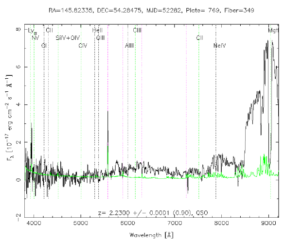
Figure 1: Observed optical spectrum of J0943+5417 from the Sloan Digital Sky Survey. The suppression of the spectrum here is a clear example of why it is difficult to correct the observed optical data.

We first correct for Galactic extinction caused by the Milky Way for the 2MASS magnitudes. This extinction is given for the u-band in the SDSS quasar catalog for each object (Schneider et al. 2007). From that value, we obtain the extinction in the 2MASS bands using the Milky Way extinction curve,

$$\frac{A_{\lambda}}{A_{B}}=\left(\frac{E(\lambda-V)}{E(B-V)}+R_{V}\right)\frac{1}{1+R_{V}},$$ (4)

where the values of color excesses, $E(\lambda-V)$, and $R_{V}=3.08$ are taken from Pei (1992). After correcting for Galactic extinction, we calculate the observed flux densities at the central $J$, $H$, and $K_{s}$ wavelengths, and obtain the rest frame monochromatic luminosities at optical bands (at $\sim$6,900Å) using Equation 3. We correct for the intrinsic dust extinction in these quasars assuming $E(B-V)=0.077$ with an SMC-like extinction curve, found by Reichard et al. (2003) to be a good approximation for LoBALs. Since FeLoBALs have higher dust extinctions than LoBALs, we possibly under-correct the intrinsic dust extinction for our targets. Finally, we extrapolate the rest-frame optical luminosities to $l_{2500}$ using the mean quasar SED of Richards et al. (2006). The parameters and intermediate results used in all these calculations are listed in Table 4. The results obtained from $J$, $H$, and $K_{s}$ bands are consistent within 20% for J0943+5417 and J1352+4239, suggesting no significant complexity in the corresponding spectra. For J1723+5553, the 2500Å luminosities extrapolated from $J$ and $H$ bands are consistent within 20%; however, the value extrapolated from the $K_{s}$ band is twice as large. It is possible that the observed $K_{s}$ band is contaminated by a strong $H_{\alpha}$ emission line. For all three objects, we use the average of the $l_{2500}$ values extrapolated from the $J$, $H$, and $K$ bands, in our following calculations.

Table 4: Rest Frame 2500Å Luminosity

Object	z	$A_{u}$	$K_{s}$	$f_{21,590\text{\AA}}$	$l_{\sim 6900\text{\AA}}$	$l_{2500}$ from $J$	$l_{2500}$ from $H$	$l_{2500}$ from $K_{s}$
			magnitude	erg cm-2 s-1Hz-1	erg s-1Hz-1	erg s-1Hz-1	erg s-1Hz-1	erg s-1Hz-1
J0943+5417	2.23	0.063	14.251	1.408$\times 10^{17}$	1.6$\times 10^{32}$	9.1$\times 10^{31}$	1.3$\times 10^{32}$	1.6$\times 10^{32}$
J1352+4239	2.04	0.055	13.861	2.002$\times 10^{17}$	2.0$\times 10^{32}$	1.5$\times 10^{32}$	1.5$\times 10^{32}$	1.8$\times 10^{32}$
J1723+5553	2.11	0.178	14.097	1.804$\times 10^{17}$	1.9$\times 10^{32}$	7.8$\times 10^{31}$	9.5$\times 10^{31}$	1.6$\times 10^{32}$

Note. — Statistics for all three objects. The redshift, $z$, and galactic extinction, $A_{u}$, are taken from Sloan Digital Sky Survey; $K_{s}$ is the observed magnitude from 2MASS; $f_{21,590}$ is the observed flux in the $K_{s}$ band; $l_{\sim 6900\text{\AA}}$ is the luminosity in the rest frame wavelengths of the $K_{s}$ band for each object; The last three columns contain the luminosity at 2,500Å as extrapolated from the $J$, $H$, and $K_{s}$ bands.

4 Results

After calculating the intrinsic monochromatic luminosities at 2500Å and 2 keV rest frame, we measure the broadband spectral index between the UV and X-ray bands, $\alpha_{\rm ox}$$=0.3838\times\log{(l_{2keV}/l_{2500})}$, and then compare our $\alpha_{\rm ox}$ values to those of the large sample of 333 normal quasars from Steffen et al. (2006). The sample was chosen to cover as much of the $l-z$ plane as possible. Other studies including FeLoBALs (Brotherton et al., 2005; Rogerson et al., 2011) found a slightly different trend. Brotherton et al. (2005) assumed a galactic column density using Schlegel et al. (1998) and found lower than expected intrinsic $\alpha_{\rm ox}$ values for their two FeLoBALs. They lie right on the bottom edge of and just below ($\Delta$$\alpha_{\rm ox}$=0.3) the scatter of expected $\alpha_{\rm ox}$ for the $l_{2500}\sim$$\alpha_{\rm ox}$ relation from Steffen et al. (2006). Rogerson et al. (2011) compared the observed $\alpha_{\rm ox}$ of their FeLoBALs with the Steffen et al. (2006) study, and found the observed $\alpha_{\rm ox}$ to be $\sim 0.48$ below the expected scatter. From this they inferred an intrinsic column density. We follow the convention of Steffen et al. (2006) and use 2500Å and 2 keV, although $\alpha_{\rm ox}$ can be defined using other optical wavelengths and X-ray energies, as shown by Young et al. (2010). In this section, we first examine the dependency of $\alpha_{\rm ox}$ on the intrinsic absorption in our FeLoBALs, using $\alpha_{\rm ox}$ calculated independently from the soft X-ray (0.2–2 keV, observed) and the hard X-ray (2–10 keV, observed) spectra. Then we analyze $\alpha_{\rm ox}$ as a function of UV and X-ray luminosities, and draw conclusions about the intrinsic column density.

4.1 Intrinsic Absorption and $\alpha_{ox}$

We first study the relation between $\alpha_{\rm ox}$ and the intrinsic absorption in Figure 2. Each sub-figure corresponds to one FeLoBAL, and shows the entire input range for intrinsic column density. The values calculated from the 2–10 keV (hard) spectrum are depicted in black, and the 0.2-2 keV (soft) spectrum are depicted by red, filled symbols. Where monochromatic luminosities at 2 keV are upper limits due to the non-detection of a source, $\alpha_{\rm ox}$ is also only an upper limit, depicted in all Figures by arrows. Included are solid lines for the expected $\alpha_{\rm ox}$$\sim l_{2500}$ relation, as found by Steffen et al. (2006), and dashed lines to depict the expected scatter.

At 2 keV the intrinsic luminosity and its uncertainty are dependent on the column density within the FeLoBAL itself, which causes intrinsic absorption that must be corrected for. We use a range $10^{20}\leq N_{H}\leq 10^{25}$ cm^-2 for intrinsic column densities since the true quantity is unknown. This gives a different value of intrinsic luminosity, and therefore $\alpha_{\rm ox}$, for each column density. The luminosities at 2500Å are extrapolated from the rest frame optical luminosities, using a normal quasar SED from Richards et al. (2006), where we have corrected both the intrinsic extinction and Galactic extinction due to dust as discussed in § 3. We find the uncertainty in the luminosities to be $\sim$20%.

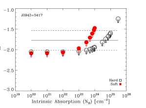
(a) J0943+5417

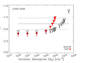
(b) J1352+4239

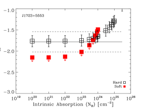
(c) J1723+5553

Figure 2: Dependence of $\alpha_{\rm ox}$ on Intrinsic Absorption ($N_{H}$). Values calculated from the 2–10 keV range are shown in black, while values calculated from the 0.2–2 keV range are shown in red filled symbols. The expected $\alpha_{\rm ox}$ from $l_{2500}$ is depicted by the solid line, with the expected scatter depicted by the dashed lines.

In the two non-detected FeLoBALs (J0943+5417 and J1352+4239), for column densities up to $1\times 10^{23}$ cm^-2, the soft limit is more stringent for $\alpha_{\rm ox}$, although the difference between the two limits diverges by $\leq 0.2$. At higher column densities, the hard spectrum is the appropriate limit to use. The divergence between the soft and hard limits is increasingly larger with increasing column density. J1723+5553 is a different story: only at $N_{H}\geq 6\times 10^{23}$ cm^-2 are the upper limits from the soft X-ray spectrum consistent with the 3$\sigma$ detection in the hard X-ray spectrum. The 3$\sigma$ detection and its uncertainties for $\alpha_{\rm ox}$ calculated from the hard X-rays are $\geq$0.3 above the upper limits given by the soft X-ray energy range for column densities $<6\times$10²³ cm^-2. Thus, the X-ray hardness ratio of J1723+5553 constrains the intrinsic column density to $N_{H}\geq 6\times 10^{23}$ cm^-2.

4.2 Monochromatic Luminosities vs. $\alpha_{\rm ox}$

Figure 3 shows the correlation between $l_{2500}$ and $\alpha_{\rm ox}$, with the best-fit linear regression for normal AGN found by Steffen et al. (2006) plotted. This relation is given by $\alpha_{\rm ox}$$=(-0.137\pm 0.008)$log$(l_{2500})+(2.638\pm 0.240)$ (Steffen et al., 2006). The solid line shows the expected $\alpha_{\rm ox}$, and the scatter is depicted by the dashed lines. Column density increases as $\alpha_{\rm ox}$ becomes less negative. The upper limits on $\alpha_{\rm ox}$ from the soft X-ray spectrum are shifted slightly to the right of the hard X-ray upper limits in Figure 3 for ease of viewing. The upper limits plotted for J0943+5417 and J1352+4239 are consistent with the normal AGN in the scatter of $\pm$0.24 for $N_{H}\geq 4\times 10^{23}$ and $N_{H}\geq 8\times 10^{23}$ cm^-2, respectively. This range falls in the column density region ($N_{H}\geq 1\times 10^{23}$) where the hard spectrum provides the appropriate upper limit. For J1723+5553, combining the constraint from X-ray hardness ratio ($\hbox{${N}_{\rm H}$}>6\times 10^{23}\hbox{cm${}^{-2}$}$), the values of $\alpha_{\rm ox}$ fall within the expected scatter if the intrinsic absorption is in the range of $6\times 10^{23}\leq N_{H}\leq 3\times 10^{24}$ cm^-2.

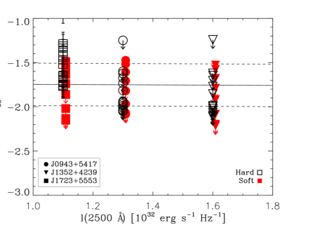
Figure 3: $\alpha_{ox}$ vs. $l_{2500\text{\AA}}$ monochromatic luminosity. Values calculated from the 2–10 keV range are shown in black, while values calculated from the 0.2–2 keV range are shown in red filled symbols and shifted to the right for clarity. The solid and dashed lines represent the mean and scatter (0.24) of the relation from Steffen et al. (2006).

Figure 4 shows the correlation between $l_{2keV}$ and $\alpha_{\rm ox}$, again with the best-fit linear regression and expected scatter, using the relation, $\alpha_{\rm ox}$$=(-0.077\pm 0.015)$log$(l_{2keV})+(0.492\pm 0.387)$, from Steffen et al. (2006). Column density increases from left to right, corresponding to rising intrinsic luminosity. For column densities $N_{H}\geq 7\times 10^{23}$ cm^-2 for J0943+5417 and $N_{H}\geq 2\times 10^{24}$ cm^-2 for J1352+4239, $\alpha_{\rm ox}$ is consistent with the normal AGN sample. The upper limits given by the soft spectrum fall within (and above) the scatter in the high column density region, where the hard spectrum gives the better constraint. Our 3$\sigma$ detection of J1723+5553 indicates that for column densities $N_{H}\leq 8\times 10^{24}$ cm^-2, J1723+5553 is consistent with the SEDs of normal AGNs.

Therefore, combining all constraints, J1723+5553 is consistent with normal AGN for column densities $6\times 10^{23}\leq N_{H}\leq 3\times 10^{24}$ cm^-2, while $\alpha_{\rm ox}$ for J0943+5417 and J1352+4239 are consistent with normal AGN for $N_{H}\geq 7\times 10^{23}$ cm^-2 and $N_{H}\geq 2\times 10^{24}$ cm^-2, respectively.

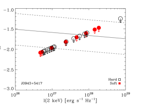
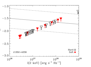
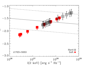
Figure 4: $\alpha_{ox}$ vs. $l_{2keV}$ monochromatic luminosity. Values calculated from the 2–10 keV range are shown in black, while values calculated from the 0.2-2 keV range are shown in red filled symbols. The solid and dashed lines represent the mean and scatter (0.387) of the relation as seen in Steffen et al. (2006).

5 Discussion

5.1 Column Densities and Intrinsic X-ray Luminosities

We find significantly high column densities for all three FeLoBALs studied, $6\times 10^{23}\leq N_{H}\leq 3\times 10^{24}$ cm^-2 for J1723+5553, $\hbox{${N}_{\rm H}$}\geq 7\times 10^{23}$ cm^-2 for J0943+5417, and $\hbox{${N}_{\rm H}$}\geq 2\times 10^{24}$ cm^-2 for J1352+4239. Only a small sample of FeLoBALs has been studied in X-rays previously. We summarize all the measurements in Table 5, which is divided into two subsamples: those that are radio loud, and those that are not. The radio loud objects tend to have lower column densities, which could be due to geometry or evolution. The X-ray emission may be linked to the jets as well as from the corona right above the central portion of the accretion disk (e.g., Miller et al., 2009). The BAL wind (see Gallagher & Everett (2007) for a detailed illustration), would then only absorb X-ray emission from the accretion disk region. We do not know for certain what complicated structure dependence for X-ray emission may exist in a radio loud FeLoBAL, but the column density results are still important and thus we include them for completeness. Our three FeLoBALs are radio quiet, and our constraints are consistent with the subsample that is not known to be radio loud. These objects in general are found to have ${N}_{\rm H}$ on the order of a few $10^{23}$ cm^-2 or higher. Notably, the most recent study by Rogerson et al. (2011) found column densities for J2215-0045 and J0300+0048 to be $\hbox{${N}_{\rm H}$}\sim 10^{24}$, with J2215-0045 just above the range we calculate for J1723+5553, but still consistent with our ${N}_{\rm H}$ for the two non-detections. The most recent calculation of column density for MrK 231 by Braito et al. (2004), using BeppSAX, found ${N}_{\rm H}$$\sim 2\times 10^{24}$ cm^-2, in agreement with all three of our objects. Green et al. (2001) cite lower column densities ($\hbox{${N}_{\rm H}$}\geq 6.5\times 10^{22}$ cm^-2), but they also noted that this is an average expected column density for a HiBAL, and that ${N}_{\rm H}$ for a LoBAL would be higher.

The fact that our 3$\sigma$ detection in J1723+5553 is in the observed 2–10 keV (rest frame 6–30 keV) hard band rather than the soft X-ray band is significant, as this is expected from highly absorbed X-ray emission from the corona above the SMBH. The non-detection of the source in the observed 0.2–2 keV (rest frame 0.6–6 keV) band is consistent with our interpretation that we detect the direct X-ray emission in the observed 2–10 keV band, as high column densities will suppress the soft X-rays more than the hard X-rays. This is further supported by the fact that none of these objects is detected, even at the 3$\sigma$ level of significance, for the broadband observed 0.2–10 keV (rest frame 0.6–30 keV) energy range. If the observed 2–10 keV spectrum is reflected or scattered into our line of sight, the X-ray spectrum will be a flat power-law, and we would also detect the source in the observed 0.2–2 keV band, which has a larger collecting area for Suzaku. Combining the measurements from this paper and those from Braito et al. (2004); Rogerson et al. (2011), it is most likely that the intrinsic ${N}_{\rm H}$ column density absorbing the X-ray emission in a radio-quiet FeLoBAL is in the range from $\sim 10^{24}$ up to $10^{25}$ cm^-2. This is about 1–2 orders of magnitude higher than the X-ray absorption range in BALQSOs ($N_{H}\sim 10^{22}-10^{24}$ cm^-2, e.g., Gallagher et al. 2006).

Using $\alpha_{\rm ox}$ to provide limits on intrinsic column density also allows us to provide limits on the intrinsic X-ray luminosity. Using the combined constraints summarized at the end of Section 4.2, the intrinsic X-ray luminosity for J0943+5417 is $l_{2{\rm\,keV}}\geq 9.8\times 10^{26}$ erg s^-1 Hz^-1; for J1352+4239 it is $l_{2{\rm\,keV}}\geq 1.7\times 10^{27}$ erg s^-1 Hz^-1; for J1723+5553 it is $4.4\times 10^{27}\leq l_{2{\rm\,keV}}\leq 1.2\times 10^{28}$ erg s^-1 Hz^-1. Compared to the normal sample of AGN from Steffen et al. (2006), these luminosities fall into the middle to high range of X-ray luminosities for normal quasars. This is predicated on the fact that we assumed an intrinsic SED for a normal AGN. The broadband luminosities for these objects in the soft band are $L_{0.6-6{\rm\,keV}}\geq 3.8\times 10^{44}$ erg s^-1, $L_{0.6-6{\rm\,keV}}\geq 6.9\times 10^{44}$ erg s^-1, and $1.8\times 10^{45}\leq L_{0.6-6{\rm\,keV}}\leq 4.9\times 10^{45}$ erg s^-1, for J0943+5417, J1352+4239, and J1723+5553, respectively. The corresponding hard band luminosities are $L_{6-30{\rm\,keV}}\geq 3.2\times 10^{44}$ erg s^-1, $L_{6-30{\rm\,keV}}\geq 5.85\times 10^{44}$ erg s^-1, and $1.5\times 10^{45}\leq L_{6-30{\rm\,keV}}\leq 4.2\times 10^{45}$ erg s^-1.

Table 5: X-ray Observations of FeLoBALs

FeLoBALs
Object	Detection	Observatory	$N_{H}$ (cm-2)	Reference
J0943+5417	no	Suzaku	$\geq 7\times 10^{23}$	This paper
J1352+4239	no	Suzaku	$\geq 2\times 10^{24}$	This paper
J1723+5553	no	Suzaku	$6\times 10^{23}-3\times 10^{24}$	This paper
SDSS J0300+0048	no	Chandra	$\geq 1.8\times 10^{24}$	Rogerson et al. (2011)
SDSS J2215-0045	no	Chandra	$\geq 3.4\times 10^{24}$	Rogerson et al. (2011)
Mrk 231	yes	BeppoSAX	$\sim 2\times 10^{24}$	Braito et al. (2004)
Q0059-2735	no	Chandra	$\geq 6.5\times 10^{22}$	Green et al. (2001)
Radio Loud FeLoBALs
Object	Detection	Observatory	$N_{H}$ (cm-2)	Reference
SDSS J1556+3517	yes	Chandra	$<9.6\times 10^{23}$	Kunert-Bajraszewska et al. (2009)
SDSS J2107-0620	yes	Chandra	$<9.6\times 10^{23}$	Kunert-Bajraszewska et al. (2009)
SDSS J1044+3656	yes	Chandra	$<9.6\times 10^{23}$	Kunert-Bajraszewska et al. (2009)
SDSS J0814+3647	yes	Chandra	$\cdots$	Miller et al. (2009)
SDSS J2107-0620	no	XMM-Newton	$4\times 10^{23}$	Wang et al. (2008)
FIRST 1044+3517	yes	Chandra	$\sim 3\times 10^{23}$	Brotherton et al. (2005)
FIRST 1556+4517	yes	Chandra	$\sim 3\times 10^{23}$	Brotherton et al. (2005)
FTM 1004+1229	yes	Chandra	$2.8\times 10^{23}$	Urrutia et al. (2005)
FTM 1036+2828	yes	Chandra	$3.8\times 10^{22}$	Urrutia et al. (2005)
FTM 0830+3759	yes	Chandra	$2.7\times 10^{22}$	Urrutia et al. (2005)

Note. — Previous studies of FeLoBALs in the X-ray. We have added column density constraints when the study provided them.

5.2 Thomson Scattering Implications

Such high column densities are interesting physically, as they are either in or on the cusp of a regime where the Thomson scattering cross-section, $\sigma_{T}=6.65\times 10^{-25}$ cm², will be large enough to scatter incident photons. Although we probe the rest frame quasar spectra in the rest frame 6–30 keV (observed 2–10 keV) band, the Klein-Nishina correction to the Thomson scattering cross section is still negligible. For J1723+5553, using the expected $\alpha_{\rm ox}$ from the $\alpha_{\rm ox}$–$l_{2kev}$ relation, the optical depth is $\tau\sim 1$. For J0934+5417 and J1352+4239, the expected $\alpha_{\rm ox}$ value from the $\alpha_{\rm ox}$–$l_{2keV}$ relation gives an intrinsic $\hbox{${N}_{\rm H}$}\sim 8.5\times 10^{24}$ cm^-2, which indicates a Thomson scattering optical depth of $\tau\sim 6$. Such a large optical depth will also significantly modulate the UV flux ($\sim$400 times dimmer); however, these objects are already more luminous in the UV than most of the AGN in the Steffen et al. (2006) study. As another check, we calculate the black hole mass of the quasars assuming they are emitting at 1/3 of the Eddington luminosity (e.g., Shankar et al. 2010). We extrapolate our rest frame luminosities to 5100Å and assume a bolometric correction of 10.33 for 5100Å (Richards et al., 2006) before using Equation 5 to find the black hole masses.

$$M_{BH}\simeq\frac{1}{3}\left(\frac{L_{Edd}}{1.5\times 10^{38}}M_{\odot}\right)\simeq\frac{3L_{bol}}{1.5\times 10^{38}}M_{\odot}$$ (5)

For the values reported here, all three FeLoBALs have $M_{BH}\sim 1.4\times 10^{8}M_{\odot}$. Even at the lower end of the column density constraints, $\hbox{${N}_{\rm H}$}\geq 6\times 10^{23}$ cm^-2, the optical depth would be $\tau\sim.4$, which would dim the intrinsic luminosity by one and a half times. At the column density corresponding to the expected $\alpha_{\rm ox}$ for J0943+5417 and J1352+4239, $\sim 8.5\times 10^{24}$ cm^-2 (from the $\alpha_{\rm ox}$–$l_{2kev}$ relation, and still within the limits for J1723+5553), the optical depth of $\tau\sim 6$ would mean the intrinsic luminosity would be increased by 400 times, giving a black hole mass of $M_{BH}\sim 3.2\times 10^{12}M_{\odot}$. Such a large mass is not a physical possibility; therefore, it is unlikely that these objects are super-luminous in the UV, and we only see the tiny fraction of Thomson scattered emission.

Since the X-ray emission region is expected to be smaller than the UV emission region from either variability (e.g., Chartas et al. 2001) or quasar microlensing (e.g., Dai et al. 2003, 2010a; Pooley et al. 2007; Morgan et al. 2008; Chartas et al. 2009) arguments, it is instead possible that the X-ray absorbing material is located between the X-ray and UV emission region and only covers the X-ray emitting region. This is consistent with the disk wind models of Gallagher & Everett (2007) and Murray et al. (1995), where an essential component of the model is the Compton thick shielding gas between the X-ray and UV emission, protecting the disk wind from being ionized by the X-ray emission. Rogerson et al. (2011) also reached a similar conclusion, where the Thomson scattering optical depth was argued to have $\tau\geq 3$ ($\geq 20$ times dimmer). In this paper, the constraint is likely more stringent with $\tau\sim 6$ ($\sim 400$ times dimmer). Aoki (2010) analyzed the UV spectrum of J1723+5553, and found the ${N}_{\rm H}$ column density in the UV wind was $\hbox{${N}_{\rm H}$}\geq 5\times 10^{17}$ cm^-2 using the curve of growth method with the unresolved Balmer absorption lines. Aoki (2010) pointed out that the covering fraction cannot be determined due to unresolved absorption lines, and assumed a covering fraction of 1. The column density would be higher than the given limit if the covering fraction is significantly less than 1. The limit derived by Aoki (2010) is seven orders of magnitude less than, but still consistent with, our X-ray column densities. If the X-ray and UV absorbing gasses are located in different regions, it can still be incorporated into both existing geometrical interpretations of FeLoBALs (e.g., Murray et al. 1995; Gallagher & Everett 2007) or evolutionary models (e.g., Fabian 1999). However, for evolutionary models the UV emission should come from the photosphere of the gas/dust cloud rather than the accretion disk. Such models have been simulated in recent studies (e.g., Casebeer et al., 2008), and support that FeLoBALs may be an evolutionary stage in the development of normal quasars.

Another explanation is that FeLoBALs have intrinsic SEDs different from normal quasars. They could be extremely X-ray weak compared to normal quasars, as in the case of the narrow-line quasar PHL 1811 (Leighly et al., 2007), or the Narrow-Line Seyfert 1 galaxy WPVS 007 (Grupe et al., 2008). This would nullify our ${N}_{\rm H}$ constraints for J0934+5417 and J1352+4239, since they are obtained by assuming a normal quasar SED. However, this would not explain J1723+5553, which we detect in the observed 2–10 keV band, but not in the observed 0.2-2 keV band. If J1723+5553 were intrinsically X-ray weak, and X-ray unabsorbed, we would expect to see a flat-line power-law slope for quasars in the hard and the soft X-ray bands. This is not consistent with our observations. In addition, the ${N}_{\rm H}$ constraint from the X-ray hardness ratio is still valid for $\hbox{${N}_{\rm H}$}\geq 6\times 10^{23}$ cm^-2 with the Thomson scattering optical depth $\tau\geq 0.4$, which could only marginally scatter the UV emission if the true ${N}_{\rm H}$ column density is close to the lower boundary.

More X-ray detections of FeLoBALs are needed so that we are not restricted by using the broadband SED constraints. It is also possible that quasar host galaxies contribute a fraction of rest frame 4000–7000Å emission; however, the contamination at this band is usually small. In addition, we correct the intrinsic dust extinction for FeLoBALs using the average dust extinction for LoBALs, which will underestimate the intrinsic flux and give less steep $\alpha_{\rm ox}$ values. A priori, it is unclear what the net effect of these two possibilities will be on the broadband flux; IR spectroscopy is needed to help resolve these issues.

5.3 AGN Kinetic Feedback

We calculate the kinetic feedback efficiency, $\epsilon_{k}=\dot{E}_{k}/L_{Bol}$, of the X-ray absorber in FeLoBALs using the location, luminosity, and ${N}_{\rm H}$ column density constraints obtained in this paper. In particular, $\dot{E}_{k}$ is the kinetic feedback power, $\dot{E}_{k}=\dot{M}v^{2}/2=4\pi\mu m_{p}f_{c}r\hbox{${N}_{\rm H}$}v^{3}$ (e.g., Moe et al. 2009), where $\mu$ is the mean molecular weight, $m_{p}$ is the proton mass, $f_{c}$, $r$, ${N}_{\rm H}$ and $v$ are the covering fraction, location, column density, and velocity of the wind, respectively, and $L_{Bol}$ is the bolometric luminosity of the quasar. If the SEDs of FeLoBALs are consistent with those of normal quasars, we obtain a reasonable $\hbox{${N}_{\rm H}$}\sim 3\times 10^{24}$ cm^-2; this is the upper end of the column density range for our 3$\sigma$ detection, and entirely consistent with our column density lower limits for the non-detections. We locate the wind between the UV and X-ray emission regions, $\sim 40r_{g}$ and $r_{g}=GM/c^{2}$, using the microlensing constraints of Dai et al. (2010a). For the covering fraction, we use the intrinsic FeLoBAL population range of 1.5% and 2.1%, depending on which model (Dai et al., 2010b) is used, and assume the quasars are emitting at a typical 0.3 Eddington limit (Shankar et al. 2010). We are left with one uncertainty, the velocity of the X-ray absorber. The velocity of the BAL wind is usually measured in the UV wind, which can reach up to $\sim 0.1c$. Since the X-ray absorbing wind is located at smaller radii than the UV absorber, its velocity can be higher than the wind velocity measured from the UV spectrum. The only velocity measurement of the X-ray absorber is from the blue-shifted X-ray absorption lines detected in a few gravitationally lensed BALQSOs (Chartas et al. 2002, 2003, 2007), and this velocity can reach 0.3–0.8$c$. Since the X-ray absorption lines are mostly detected in mini-BALs, we could possibly be looking through the edge of the wind, where the wind can be by fully accelerated. Thus, we consider the X-ray absorption line as providing an upper limit, and assume our wind velocity is 0.1–0.3$c$, between the estimates from the two methods. We find the feedback efficiency, $\epsilon_{k}$, for FeLoBALs is in the range (outflow velocity dependent) of either 0.2%–4.8% for a covering fraction of 1.5%, or 0.3%–6.9% for a covering fraction of 2.1%. To reach the minimum of 5% required to explain the co-evolution between black holes and host galaxies (e.g., Silk & Rees 1998; Granato et al. 2004; Hopkins et al. 2005), with the other variables given here, we need a column density of ${N}_{\rm H}$$\geq 8\times 10^{25}$ cm^-2 or ${N}_{\rm H}$$\geq 6\times 10^{25}$ cm^-2 for low velocity wind with the different covering fractions. These are consistent with our lower limits on column density for the two non-detections, but out of reach for J1723+5553. However, for the high end of the conservative wind velocity range, only ${N}_{\rm H}$$\geq 3\times 10^{24}$ and ${N}_{\rm H}$$\geq 2\times 10^{24}$ are needed for $f_{c}=$1.5% and 2.1%, respectively. Both of these column densities are consistent with the results for J1723+5553, and thus it is likely that FeLoBALs can contribute to AGN feedback. This becomes even more likely when models like Hopkins & Elvis (2010) are considered. They describe a “two-stage” feedback process, where a weak wind from the central engine energizes a hot, diffuse interstellar medium, which is then amplified when it it hits instabilities in a cold cloud within the host. This amplification outside of the central engine requires feedback efficiency as small as 0.5%. The BAL wind in FeLoBALs, therefore, is a promising candidate for the feedback process responsible for the co-evolution between black holes and host galaxies. More measurements of $N_{H}$ are needed to further quantify how important the contributions are from FeLoBALs and BALQSOs to kinetic feedback efficiency.

References

- Allen et al. (2010) Allen, J. T., Hewett, P. C., Maddox, N., Richards, G. T., & Belokurov, V. 2010, MNRAS, 1715
- Aoki (2010) Aoki, K. 2010, PASJ, 62, 1333
- Becker et al. (1995) Becker, R. H., White, R. L., & Helfand, D. J. 1995, ApJ, 450, 559
- Braito et al. (2004) Braito, V., et al. 2004, A&A, 420, 79
- Brotherton et al. (2005) Brotherton, M. S., Laurent-Muehleisen, S. A., Becker, R. H., Gregg, M. D., Telis, G., White, R. L., & Shang, Z. 2005, AJ, 130, 2006
- Casebeer et al. (2008) Casebeer, D., Baron, E., Leighly, K., Jevremovic, D., & Branch, D. 2008, ApJ, 676, 857
- Chartas et al. (2001) Chartas, G., Dai, X., Gallagher, S. C., Garmire, G. P., Bautz, M. W., Schechter, P. L., & Morgan, N. D. 2001, ApJ, 558, 119
- Chartas et al. (2002) Chartas, G., Brandt, W. N., Gallagher, S. C., & Garmire, G. P. 2002, ApJ, 579, 169
- Chartas et al. (2003) Chartas, G., Brandt, W. N., & Gallagher, S. C. 2003, ApJ, 595, 85
- Chartas et al. (2007) Chartas, G., Eracleous, M., Dai, X., Agol, E., & Gallagher, S. 2007, ApJ, 661, 678
- Chartas et al. (2009) Chartas, G., Kochanek, C. S., Dai, X., Poindexter, S., & Garmire, G. 2009, ApJ, 693, 174
- Condon et al. (1998) Condon, J. J., Cotton, W. D., Greisen, E. W., Yin, Q. F., Perley, R. A., Taylor, G. B., & Broderick, J. J. 1998, AJ, 115, 16
- Dai et al. (2003) Dai, X., Chartas, G., Agol, E., Bautz, M. W., & Garmire, G. P. 2003, ApJ, 589, 100
- Dai et al. (2004) Dai, X., Chartas, G., Eracleous, M., & Garmire, G. P. 2004, ApJ, 605, 45
- Dai et al. (2008) Dai, X., Shankar, F., & Sivakoff, G. R. 2008, ApJ, 672, 108
- Dai et al. (2010a) Dai, X., Kochanek, C. S., Chartas, G., Kozłowski, S., Morgan, C. W., Garmire, G., & Agol, E. 2010a, ApJ, 709, 278
- Dai et al. (2010b) Dai, X., Shankar, F., & Sivakoff, G. R. 2010b, MNRAS, submitted, arXiv:1004.0700
- Dickey & Lockman (1990) Dickey, J. M. & Lockman, F. J. 1990, ARAA, 28, 215
- Elvis (2000) Elvis, M. 2000, ApJ, 545, 63
- Fabian (1999) Fabian, A. C. 1999, MNRAS, 308, L39
- Farrah et al. (2007) Farrah, D., Lacy, M., Priddey, R., Borys, C., & Afonso, J. 2007, ApJ, 662, L59
- Farrah et al. (2010) Farrah, D., et al. 2010, ApJ, 717, 868
- Gallagher et al. (2002a) Gallagher, S. C., Brandt, W. N., Chartas, G., & Garmire, G. P. 2002a, ApJ, 567, 37
- Gallagher et al. (2002b) Gallagher, S. C., Brandt, W. N., Chartas, G., Garmire, G. P., & Sambruna, R. M. 2002b, ApJ, 569, 655
- Gallagher et al. (2006) Gallagher, S. C., Brandt, W. N., Chartas, G., Priddey, R., Garmire, G. P., & Sambruna, R. M. 2006, ApJ, 644, 709
- Gallagher & Everett (2007) Gallagher, S. C., & Everett, J. E. 2007, The Central Engine of Active Galactic Nuclei, 373, 305
- Ganguly & Brotherton (2008) Ganguly, R., & Brotherton, M. S. 2008, ApJ, 672, 102
- Graham et al. (2011) Graham, A. W., Onken, C. A., Athanassoula, E., & Combes, F. 2011, MNRAS, 48
- Granato et al. (2004) Granato, G. L., De Zotti, G., Silva, L., Bressan, A., & Danese, L. 2004, ApJ, 600, 580
- Green et al. (2001) Green, P. J., Aldcroft, T. L., Mathur, S., Wilkes, B. J., & Elvis, M. 2001, ApJ, 558, 109
- Grupe et al. (2008) Grupe, D., Leighly, K. M., & Komossa, S. 2008, AJ, 136, 2343
- Gültekin et al. (2009) Gültekin, K., et al. 2009, ApJ, 698, 198
- Hall et al. (2010) Hall, P. B., Anosov, K., White, R. L., Brandt, W. N., Gregg, M. D., Gibson, R. R., Becker, R. H., & Schneider, D. P. 2010, arXiv:1010.3728
- Hopkins & Elvis (2010) Hopkins, P. F., & Elvis, M. 2010, MNRAS, 401, 7
- Hopkins et al. (2005) Hopkins, P. F., Hernquist, L., Cox, T. J., Di Matteo, T., Martini, P., Robertson, B., & Springel, V. 2005, ApJ, 630, 705
- Joye & Mandel (2003) Joye, W. A. & Mandel, E. 2003, ASPC, 295, 498
- Knigge et al. (2008) Knigge, C., Scaringi, S., Goad, M. R., & Cottis, C. E. 2008, MNRAS, 386, 1426
- Koyama et al. (2007) Koyama, K., et al. 2007, PASJ, 59, 23
- Kunert-Bajraszewska et al. (2009) Kunert-Bajraszewska, M., Siemiginowska, A., Katarzyński, K., & Janiuk, A. 2009, ApJ, 705, 1356
- Leighly et al. (2007) Leighly, K. M., Halpern, J. P., Jenkins, E. B., Grupe, D., Choi, J., & Prescott, K. B. 2007, ApJ, 663, 103
- Lípari et al. (2009) Lípari, S., et al. 2009, NMRAS, 392, 1295
- Maddox et al. (2008) Maddox, N., Hewett, P. C., Warren, S. J., & Croom, S. M. 2008, MNRAS, 386, 1605
- Miller et al. (2009) Miller, B. P., Brandt, W. N., Gibson, R. R., Garmire, G. P., & Shemmer, O. 2009, ApJ, 702, 911
- Mitsuda et al. (2007) Mitsuda, K., et al. 2007, PASJ, 59, 1
- Moe et al. (2009) Moe, M., Arav, N., Bautista, M. A., & Korista, K. T. 2009, ApJ, 706, 525
- Morgan et al. (2008) Morgan, C. W., Kochanek, C. S., Dai, X., Morgan, N. D., & Falco, E. E. 2008, ApJ, 689, 755
- Murray et al. (1995) Murray, N., Chiang, J., Grossman, S. A., & Voit, G. M. 1995, ApJ, 451, 498
- Pei (1992) Pei, Y. C. 1992, ApJ, 395, 130
- Pooley et al. (2007) Pooley, D., Blackburne, J. A., Rappaport, S., & Schechter, P. L. 2007, ApJ, 661, 19
- Reeves & Turner (2000) Reeves, J. N., & Turner, M. J. L. 2000, MNRAS, 316, 234
- Reichard et al. (2003) Reichard, T. A., Richards, G. T., Hall, P. B., Schneider, D. P., Vanden Berk, D. E., Fan, X., York, D. G., Knapp, G. R., & Brinkmann, J. 2003, AJ, 126, 2594
- Richards et al. (2006) Richards, G. T., Lacy, M., Storrie-Lombardi, L. J., et al. 2006, APJS, 166, 470
- Rogerson et al. (2011) Rogerson, J. A., Hall, P. B., Snedden, S. A., Brotherton, M. S., & Anderson, S. F. 2011, New A, 16, 128
- Saez et al. (2008) Saez, C., Chartas, G., Brandt, W. N., Lehmer, B. D., Bauer, F. E., Dai, X., & Garmire, G. P. 2008, AJ, 135, 1505
- Scannapieco & Oh (2004) Scannapieco, E., & Oh, S. P. 2004, ApJ, 608, 62
- Schlegel et al. (1998) Schlegel, D. J., Finkbeiner, D. P., & Davis, M. 1998, ApJ, 500, 525
- Schneider et al. (2007) Schneider, D. P., et al. 2007, AJ, 134, 102
- Shankar et al. (2008a) Shankar, F., Dai, X., & Sivakoff, G. R. 2008a, ApJ, 687, 859
- Shankar et al. (2008b) Shankar, F., Cavaliere, A., Cirasoulo, M., & Maraschi, L. 2008b, ApJ, 676,131
- Shankar et al. (2010) Shankar, F., Sivakoff, G. R., Vestergaard, M., & Dai, X. 2010, MNRAS, 401, 1869
- Silk & Rees (1998) Silk, J., & Rees, M. J. 1998, A&A, 331, L1
- Silk & Nusser (2010) Silk, J., & Nusser, A. 2010, arXiv:1004.0857
- Sprayberry & Foltz (1992) Sprayberry, D. & Foltz, C. B. 1992, ApJ, 390, 39
- Steffen et al. (2006) Steffen, A. T., Strateva, I., Brandt, W. N., Alexander, D. M., Koekemoer, A. M., Lehmer, B. D., Schneider, D. P., & Vignali, C. 2006, AJ, 131, 2826
- Streblyanska et al. (2010) Streblyanska, A., Barcons, X., Carrera, F. J., & Gil-Merino, R. 2010, A&A, 515, A2
- Trump et al. (2006) Trump, J. R., et al. 2006, ApJs, 165, 1
- Turner & Kraemer (2003) Turner, T. J., & Kraemer, S. B. 2003, ApJ, 598, 916
- Urrutia et al. (2005) Urrutia, T., Lacy, M., Gregg, M. D., & Becker, R. H. 2005, ApJ, 627, 75
- Urrutia et al. (2009) Urrutia, T., Becker, R. H., White, R. L., Glikman, E., Lacy, M., Hodge, J., & Gregg, M. D. 2009, ApJ, 698, 1095
- Wang et al. (2008) Wang, J., Jiang, P., Zhou, H., Wang, T., Dong, X., & Wang, H. 2008, ApJ, 676, L97
- Weymann et al. (1991) Weymann, R. J., Morris, S. L., Foltz, C. B., & Hewett, P. C. 1991, ApJ, 373,23
- Yamaguchi et al. (2006) Yamaguchi, H., Nakajima, H., Koyama, K., Tsuru, T. G., Matsumoto, H., Tawa, N., Tsunemi, H., Hayashida, K., Torii, K., Namiki, M., Katayama, H., Dotani, T., Ozaki, M., Murakami, H., & Miller, E. 2006, SPIE, 6266, 626642
- Young et al. (2010) Young, M., Elvis, M., & Risaliti, G. 2010, ApJ, 708, 1388