Lost and found: The missing diabolical points in the Fe₈ molecular magnet

Abstract

Certain diabolical points in the tunneling spectrum of the single-molecule magnet Fe₈ were previously believed to be have been eliminated as a result of a weak fourth-order anisotropy. As shown by Bruno, this is not so, and the points are only displaced in the magnetic field space along the medium anisotropy direction. The previously missing points are numerically located by following the lines of the Berry curvature. The importance of an experimental search for these rediscovered points is discussed.

The purpose of this note is to report on a numerical search of certain diabolical points (DP’s) in the energy spectrum of the single-molecule magnet (also known as a molecular magnet or nanomagnet) Fe₈ that were earlier believed to be missing, but are in fact not so bruno . Several other DP’s have been seen experimentally in Fe₈ werns , and their observation provides the best evidence of spin orientation tunneling between deep levels in all single-molecule magnets studied to date. Observation of even some of the missing DP’s would strengthen our understanding of Fe₈ substantially.

For a system whose Hamiltonian depends on some parameter, a DP is a point in parameter space where two (or more) energy levels are degenerate bw84 . In Fe₈, the parameter is the static applied magnetic field, and the locations of the DP’s so far observed (as well as many other experimental measurements) are well described by the anisotropy Hamiltonian,

$${\cal H}=k_{1}J_{x}^{2}+k_{2}J_{y}^{2}-C(J_{+}^{4}+J_{-}^{4})-g\mu_{B}{\bf J}\cdot{\bf H}.$$ (1)

Here ${\bf J}=(J_{x},J_{y},J_{z})$ is the spin, ${\bf H}$ is an external magnetic field, $g$ is a g-factor, $\mu_{B}$ is the Bohr magneton, and $k_{1}$, $k_{2}$, and $C$ are anisotropy coefficients. Experimentally, $J=10$, $k_{1}\simeq 0.338$ K, $k_{2}\simeq 0.246$ K, $C\simeq 29\,\mu$K, and $g\simeq 2$. The DP’s can be understood as arising when tunneling between two states with (nearly) oppositely oriented magnetic moment is quenched because of destructive interference between instantons (spin tunneling trajectories) gargepl ; loss_and_henley .

The model Hamiltonian (1) was first analyzed in 1993 gargepl with $C=0$, and it was found that for ground state tunneling it had 10 DP’s along the positive $H_{x}$ axis, corresponding to $J=10$. In reality only 4 DP’s are seen werns , which was explained in Ref. ekag as follows. When $C\neq 0$, we get two new (but noninterfering) instantons, which are discontinuous at the end points. One of these instantons has the least action when $H_{x}$ exceeds a certain value $H^{*}$, and since this instanton has no interfering partner, there are no more DP’s for $H_{x}>H^{*}$. For the values of the anisotropy coefficients quoted above, $H^{*}$ lies just beyond the location of the fourth DP, which explains why the last six DP’s are not seen in experiment or by direct numerical diagnolization of Eq. (1). We can further check this picture by decreasing $C$ so as to make $H^{*}$ larger. It is seen that as this happens, one successively sees six and then eight, and finally all ten DP’s, all in accord with direct numerical diagonalization results ekag .

However, as shown by Bruno bruno , the above picture, though correct, is incomplete. For any energy level, the sum of the Chern numbers for all DPs involving that level is a topological invariant as parameters like $k_{1}$, $k_{2}$, or $C$ are varied. Since DP’s in any system are generically simple, we expect this to be so in Fe₈ also, and the Chern number for any one DP should be $\pm 1$ whether $C=0$ or $C\neq 0$. Hence the six missing DP’s must be present elsewhere in magnetic field space. A similar conclusion applies to the DP’s associated with tunneling between other pairs of levels ekag01 . For tunneling between the ground states, the DP’s merely move off the x axis into the xy plane. For the higher energy levels, they move off the xz plane into the full three dimensional ${\bf H}$ space. This point can also be understood by noting that for a system with purely four-fold symmetry ($k_{2}=k_{1}$, $C\neq 0$), the ground state DP’s lie on the $\pm{\bf{\hat{x}}}\pm{\bf{\hat{y}}}$ axes, while for the excited states they lie in the planes formed by these axes and the ${\bf{\hat{z}}}$ axis cpag . When both two-fold and four-fold anisotropies are present ($k_{2}\neq k_{1}$, $C\neq 0$), it is then not surprising that the location of some of the DP’s is also intermediate bruno .

Observation of these rediscovered DPs would be interesting in itself, and also provide an important test of the validity of the model (1) vs. other models leuen that add extra 6th and 8th order anisotropies because the location of the DPs is very sensitive to the higher order anisotropies. With this motivation, we have undertaken a search for the DP’s for the ground state and some of the excited states. We stress that the key insight that these points should exist in the first place is due to Bruno, and our contribution is only to find their specific locations. Neverthless, finding them is not without challenge as we discuss next.

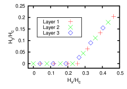
Figure 1: Diabolical points of Fe₈ corresponding to tunneling from the Zeeman level $m=-10$ to $m=10$ (layer 1), to $m=9$ (layer 2), and to $m=8$ (layer 3), all projected onto the xy plane. $H_{c}=2k_{1}J/g\mu_{B}$.

A direct search for the DPs by numerical minimization of the energy differences fails because the energy surface is like a golf course with rolling hills on which the DPs are the holes. Because the holes are so localized, unless one starts close to one of them by luck, any numerical algorithm will in general simply head for the valleys of the course and miss the holes entirely. Because ${\cal H}$ is not real for general ${\bf H}$, we also cannot use the method of Ref. cpag , which is to corral the DPs by using the Herzberg and Longuet-Higgins theorem hlh63 to find and successively bisect a sign-reversing circuit. We therefore proceed as follows. Let us denote the eigenstates and eigenvalues of Eq. (1) for fixed ${\bf H}$ by $|n({\bf H})\rangle$ and $E_{n}({\bf H})$, $n=1,\ 2,\ldots,21$, and order them so that $E_{n}\geq E_{n-1}$ for every ${\bf H}$. Except at degeneracies (the DPs), the Berry curvature for the $n$th level is defined by berry

$${\bf B}_{n}=-{\rm Im}\sum_{n^{\prime}\neq n}{\langle n|\boldsymbol{\nabla}_{{\bf H}}{\cal H}|n^{\prime}\rangle\times\langle n^{\prime}|\boldsymbol{\nabla}_{{\bf H}}{\cal H}|n\rangle\over(E_{n^{\prime}}-E_{n})^{2}}.$$ (2)

Table 1: Locations of selected diabolical points

$(m,m^{\prime})$	Layer	$(h_{x},h_{y},h_{z})$
$(-10,10)$	1	$(0.0404,0,0)$
		$(0.1207,0,0)$
		$(0.2011,0,0)$
		$(0.2565,0,0)$
		$(0.3139,\pm 0.0642,0)$
		$(0.3875,\pm 0.1334,0)$
		$(0.4656,\pm 0.2043,0)$
$(-10,9)$	2	$(0,0,0.0426)$
		$(0.0787,0,0.0426)$
		$(0.1568,0,0.0427)$
		$(0.2276,0,0.0427)$
		$(0.2893,\pm 0.0447,0.0427)$
		$(0.3594,\pm 0.1109,0.0427)$
		$(0.4340,\pm 0.1788,0.0427)$
$(-10,8)$	3	$(0.0385,0,0.0853)$
		$(0.1150,0,0.0853)$
		$(0.1892,0,0.0853)$
		$(0.2650,\pm 0.0268,0.0854)$
		$(0.3326,\pm 0.0900,0.0854)$
		$(0.4038,\pm 0.1548,0.0854)$
$(-9,9)$	1	$(0.0384,0,0)$
		$(0.1147,0,0)$
		$(0.1889,0,0)$
		$(0.2651,\pm 0.0261,0)$
		$(0.3325,\pm 0.0891,0)$
		$(0.4034,\pm 0.1535,0)$
$(-8,8)$	1	$(0.0365,0,0)$
		$(0.1089,0,0)$
		$(0.1805,0,0)$
		$(0.2339,0,0)$
		$(0.2831,\pm 0.0511,0)$
		$(0.3468,\pm 0.1092,0)$

Further, the Chern number associated with a degeneracy is given by

$$Q_{n}=-{1\over 2\pi}\oint_{S}{\bf B}_{n}\cdot d^{2}{\bf s},$$ (3)

where the integral is independent of the choice of the surface $S$, as long as it encloses the degeneracy, since $\boldsymbol{\nabla}_{{\bf H}}\cdot{\bf B}_{n}=0$ away from the degeneracy. The Chern number is always an integer, and for a simple double degeneracy, it equals $\pm 1$. In other words, near a DP, ${\bf B}_{n}$ has the form of a monopole field with flux equal to $\pm 2\pi$. Hence, to find the DPs, we numerically evaluate ${\bf B}_{n}$ for an initial ${\bf H}$, and follow the lines of ${\bf B}_{n}$ in the direction of increasing strength until we hit a monopole. Since the number of DPs where levels $n$ and $n+1$ are degenerate is topologically fixed and known, all the DPs can be found by taking sufficiently many initial values of ${\bf H}$. The DPs for successive pairs of levels occur in layers, with $H_{z}$ essentially constant in a layer. With ${\bf h}\equiv g\mu_{B}{\bf H}/2k_{1}J$, the first three layers are at $h_{z}=0$ (exactly), $0.0427$, and $0.0854$. It should be noted, however, that in a given layer, one can have DP’s corresponding to tunneling between levels with different pairs of Zeeman quantum numbers. For example, layer 1 contains points corresponding to tunneling between $m=-10\leftrightarrow 10$, $-9\leftrightarrow 9$, $-8\leftrightarrow 8$, etc. Likewise, layer 2 contains points corresponding to tunneling between $m=-10\leftrightarrow 9$, $-9\leftrightarrow 8$, $-8\leftrightarrow 7$, etc. In Table 1, we show the DP’s for $(-10\leftrightarrow 10)$ $(-10\leftrightarrow 9)$, $(-10\leftrightarrow 8)$, $(-9\leftrightarrow 9)$, and $(-8\leftrightarrow 8)$ tunneling. For the first three of these pairs of levels, the projections of the DP’s onto the xy plane are shown in Fig. 1. We note that it is just these three pairs of levels for which tunnel splittings were reported in Ref. werns . Hoewever, except for the ground pair of levels (layer 1), not even all the DP’s on the x axis are found there.

In the rest of this note, we discuss the form of the Berry curvature near a DP in more detail. For simplicity, we will divide ${\cal H}$ by $k_{1}J^{2}$. Since $\boldsymbol{\nabla}_{{\bf H}}{\cal H}$ and $E_{n}$ are both divided by this factor, it follows from Eq. (2) that ${\bf B}_{n}$ is unchanged. With this preliminary remark, let us suppose that $E_{n}=E_{n-1}\equiv E_{n,n-1}$ at ${\bf h}={\bf h}_{n,n-1}$, and denote

$${\bf r}={\bf h}-{\bf h}_{n,n-1}.$$ (4)

Further, let us make a particular choice of the two degenerate states at ${\bf r}=0$, and denote them by $|a\rangle$ and $|b\rangle$, with $\langle b|a\rangle=0$. (Any orthogonal linear combination of $|a\rangle$ and $|b\rangle$ would also work.) It suffices to truncate the Hamiltonian to this two dimensional subspace since the sum in Eq. (2) is dominated by degenerate states. Hence, at ${\bf r}=0$, we have

$${\cal H}=E_{n,n-1}\begin{pmatrix}1&0\\ 0&1\\ \end{pmatrix}.$$ (5)

For small enough ${\bf r}$, we can take $|a\rangle$ and $|b\rangle$ to be unchanged, so

$$\boldsymbol{\nabla}_{{\bf h}}{\cal H}=-{2\over J}\begin{pmatrix}{\bf J}_{aa}&{\bf J}_{ab}\\ {\bf J}_{ba}&{\bf J}_{bb}\end{pmatrix},$$ (6)

where ${\bf J}_{aa}=\langle a|{\bf J}|a\rangle$ etc. Next, let us define ${\bf J}_{aa}+{\bf J}_{bb}=J{\bf t}$, ${\bf J}_{aa}-{\bf J}_{bb}=J{\bf u}$, ${\bf J}_{ab}=J({\bf v}+i{\bf w})/2$, where ${\bf t}$, ${\bf u}$, ${\bf v}$, and ${\bf w}$ are real vectors. In terms of these vectors, we have

$${\cal H}=-{{\bf t}\cdot{\bf r}\over J}-\begin{pmatrix}{\bf u}\cdot{\bf r}&({\bf v}+i{\bf w})\cdot{\bf r}\\ ({\bf v}-i{\bf w})\cdot{\bf r}&-{\bf u}\cdot{\bf r}\end{pmatrix},$$ (7)

where we have ignored the constant $E_{n,n-1}$. Similarly ignoring the overall shift $-{\bf t}\cdot{\bf r}/J$, the eigenvalues of this matrix are $\pm\epsilon({\bf r})$, with

$$\epsilon({\bf r})=[({\bf u}\cdot{\bf r})^{2}+({\bf v}\cdot{\bf r})^{2}+({\bf w}\cdot{\bf r})^{2}]^{1/2}.$$ (8)

To write the eigenvectors compactly, we define

$$\cos\theta({\bf r}) = {\bf u}\cdot{\bf r}/\epsilon({\bf r}),$$ (9)

$$\sin\theta({\bf r})e^{i\varphi({\bf r})} = ({\bf v}+i{\bf w})\cdot{\bf r}/\epsilon({\bf r}).$$ (10)

The eigenvectors are then

$$|-\rangle=\begin{pmatrix}\cos\textstyle{1\over 2}\theta\\ \sin\textstyle{1\over 2}\theta e^{-i\varphi}\end{pmatrix},\quad|+\rangle=\begin{pmatrix}\sin\textstyle{1\over 2}\theta\\ -\cos\textstyle{1\over 2}\theta e^{-i\varphi}\end{pmatrix}.$$ (11)

Further abbreviating $c=\cos{1\over 2}\theta$ and $s=\sin{1\over 2}\theta$, and ${\bf g}=\langle+|\boldsymbol{\nabla}_{{\bf h}}{\cal H}|-\rangle$, we have

$${\bf g}=-2cs{\bf u}-s^{2}e^{-i\varphi}({\bf v}+i{\bf w})+c^{2}e^{i\varphi}({\bf v}-i{\bf w}).$$ (12)

It then follows that

$${\bf g}\times{\bf g}^{*}=2i[\cos\theta({\bf v}\times{\bf w}) + \sin\theta\cos\varphi({\bf w}\times{\bf u}){\hskip 28.45274pt}$$ (13)

$$\!\!\!\!{}+\sin\theta\sin\varphi({\bf u}\times{\bf v})],$$

so that for the level labeled ${+}$,

$${\bf B}_{+} = {-1\over 2\epsilon^{3}({\bf r})}\left[({\bf u}\cdot{\bf r})({\bf v}\times{\bf w})+({\bf v}\cdot{\bf r})({\bf w}\times{\bf u})\right.$$ (14)

$${\hskip 93.89418pt}\left.{}+({\bf w}\cdot{\bf r})({\bf u}\times{\bf v})\right]$$

$$= {-1\over 2\epsilon^{3}({\bf r})}\left[{\bf u}\cdot({\bf v}\times{\bf w})\right]{\bf r}.$$

This is clearly of monopole form with appropriately scaled and sheared axes. It is not difficult to show that ${\bf B}_{-}=-{\bf B}_{+}$ and that $\boldsymbol{\nabla}\cdot{\bf B}_{+}=0$.

To find the Chern number, we must evaluate the integral

$$Q_{\pm}=-{1\over 2\pi}\oint_{S}{\bf B}_{\pm}\cdot d^{2}{\bf s}$$ (15)

for a suitable surface $S$. Let us take $S$ to be the surface of the parallepiped with vertices at $(\pm{\bf u}^{*},\pm{\bf v}^{*},\pm{\bf w}^{*})$, where ${\bf u}^{*}$, ${\bf v}^{*}$, and ${\bf w}^{*}$ are the reciprocal vectors

$${\bf u}^{*}={\displaystyle{{\bf v}\times{\bf w}\over\Omega}},\quad{\bf v}^{*}={\displaystyle{{\bf w}\times{\bf u}\over\Omega}},\quad{\bf w}^{*}={\displaystyle{{\bf u}\times{\bf v}\over\Omega}};$$ (16)

$$\Omega={\bf u}\cdot({\bf v}\times{\bf w}).$$ (17)

Then ${\bf u}\cdot{\bf u}^{*}=1$, ${\bf u}\cdot{\bf v}^{*}={\bf u}\cdot{\bf w}^{*}=0$, etc. Let us consider the integral over the face of the parallepiped that has edges along ${\bf v}^{*}$ and ${\bf w}^{*}$, and thus has a normal parallel to $+{\bf u}$ (the others have normals along $-{\bf u}$, $\pm{\bf v}$, and $\pm{\bf w}$). On this face, we may parametrize ${\bf r}$ as

$${\bf r}={\bf u}^{*}+\alpha{\bf v}^{*}+\beta{\bf w}^{*},$$ (18)

where $-1\leq\alpha\leq 1$, $-1\leq\beta\leq 1$. Then, since the area of this face is $4|{\bf v}^{*}\times{\bf w}^{*}|=4|{\bf u}|/\Omega$,

$$d^{2}{\bf s}={{\bf u}\over\Omega}d\alpha\,d\beta.$$ (19)

Finally, ${\bf u}\cdot{\bf r}=1$, ${\bf v}\cdot{\bf r}=\alpha$, and ${\bf w}\cdot{\bf r}=\beta$. Thus, the contribution from this face to $Q_{\pm}$ is given by

$$\pm{1\over 4\pi}\int_{-1}^{1}\int_{-1}^{1}{d\alpha\,d\beta\over(1+\alpha^{2}+\beta^{2})^{3/2}}=\pm{1\over 6}.$$ (20)

(The integral is elementary, and can be performed by standard trigonometric substitutions.) The contributions from the other faces are identical, so

$$Q_{\pm}=\pm 1.$$ (21)

Thus the Chern number associated with the lower energy level is always $-1$ irrespective of the details, and this is why the sum of the numbers for a given energy level cannot be altered by varying the anisotropy parameters.

The reader cannot have failed to notice the regularity of the DP pattern for the present problem. This is in sharp contrast to the generic situation where no pattern is expected apart from a general scaling of the density with energy bw84 . The reason for this regularity is unclear to us.

This work is supported by the NSF via grant no. PHY-0854896.

References

- (1) P. Bruno, Phys. Rev. Lett. 96, 117208 (2006).
- (2) W. Wernsdorfer and R. Sessoli, Science 284, 133 (1999).
- (3) M. V. Berry and M. Wilkinson, Proc. Roy. Soc. London A 392, 15 (1984).
- (4) A. Garg, Europhys. Lett. 22, 205 (1993).
- (5) D. Loss, D. P. DiVincenzo, and G. Grinstein, Phys. Rev. Lett. 69, 3232 (1992); J. von Delft and C. L. Henley, ibid 69, 3236 (1992).
- (6) Ersin Keçecioğlu and A. Garg, Phys. Rev. Lett. 88, 237205 (2002); Phys. Rev. B 67, 054406 (2003).
- (7) J. Villain and A. Fort, Eur. Phys. J. B 17, 69 (2000). Ersin Keçecioğlu and A. Garg, Phys. Rev. B 63, 064422 (2001);
- (8) Chang-Soo Park and A. Garg, Phys. Rev. B 65, 064411 (2002).
- (9) G. Herzberg and H. C. Longuet-Higgins, Discuss. Farady Soc. 35, 77 (1963).
- (10) M. N. Leuenberger and D. Loss, Phys. Rev. B 61, 12200 (2000). The relative merits of this proposal vs. Eq. (1) are discussed in Ersin Keçecioğlu and A. Garg, Phys. Rev. B 76, 134405 (2007).
- (11) M. V. Berry, Proc. Roy. Soc. London A 392, 45 (1984).