How old are the stars in the halo of NGC 5128 (Centaurus A)?

Abstract

Context. NGC 5128 (Centaurus A) is, at the distance of just 3.8 Mpc, the nearest easily observable giant elliptical galaxy. Therefore it is the best target to investigate the early star formation history of an elliptical galaxy.

Aims. Our aims are to establish when the oldest stars formed in NGC 5128, and whether this galaxy formed stars over a long period.

Methods. We compare simulated colour-magnitude diagrams with the deep ACS/HST photometry. The simulations assume in input either the observed metallicity distribution function, based on the colour distribution of the upper red giant branch stars, or the closed box chemical enrichment. Simulations are constructed for single age bursts using BASTI evolutionary isochrones; more complex star formation histories are constructed as well by combining several individual simulations. Comparisons with data are made by fitting the whole colour-magnitude diagram as well as the the luminosity functions in $V$ and $I$ band. In addition we inspect carefully the red clump and asymptotic giant branch bump luminosities and number counts, since these features are the primary constraints on the ages of the observed stars.

Results. We find that that the observed colour-magnitude diagram can be reproduced satisfactorily only by simulations that have the bulk of the stars with ages in excess of $\sim 10$ Gyr, and that the alpha-enhanced models fit the data much better than the solar scaled ones. Data are not consistent with extended star formation over more than $3-4$ Gyr. Two burst models, with 70-80% of the stars formed $12\pm 1$ Gyr ago and with 20-30% younger contribution with $2-4$ Gyr old stars provide the best agreement with the data. The old component spans the whole metallicity range of the models ($Z=0.0001-0.04$), while for the young component the best fitting models indicate higher minimum metallicity ($\sim 1/10-1/4$ Z_⊙).

Conclusions. The bulk of the halo stars in NGC 5128 must have formed at redshift $z\ga 2$ and the chemical enrichment was very fast, reaching solar or even twice-solar metallicity already for the $\sim 11-12$ Gyr old population. The minor young component, adding $\sim 20-30$% of the stars to the halo, and contributing less than 10% of the mass, may have resulted from a later star formation event $\sim 2-4$ Gyr ago.

1 Introduction

NGC 5128 (Centaurus A) is by far the nearest easily observable giant E galaxy and the centrally dominant object in the Centaurus group of galaxies (Karachentsev 2005). At D=3.8 Mpc (Harris et al. 2010), it is more than 2 magnitudes closer than the ellipticals in the Leo group and 3 magnitudes closer than the Virgo cluster. As such, it offers an unparalleled opportunity for studying the nature of stellar populations in a large elliptical. Particularly interesting is the old-halo component whose basic properties (age distribution, metallicity distribution, star formation history) are difficult to measure in detail for galaxies beyond the Local Group.

In Paper I (Rejkuba et al. 2005), we presented HST ACS/WFC photometry of the stars in an outer-halo field of NGC 5128. The photometric limits of the data, resulting from 12 full-orbit exposures in each of the F606W and F814W filters, were deep enough to reveal both the old red-giant branch (RGB) to its reddest, most metal-rich extent, and the core-helium-burning “red clump” or horizontal branch (RC or HB) stars. The main purpose of our deep ACS/WFC photometric program was to make a first attempt at directly measuring the earliest star formation history in this keystone galaxy, because the HB is the most luminous stellar component that can unambiguously reveal very old populations. Previous work with the HST/WFPC2 camera which probed the brightest $\sim 2$ magnitudes of the RGB at other locations in the mid- and outer-halo (Harris et al. 1999; Harris & Harris 2000, 2002) indicated that the stellar population in these fields is dominated by normal, old, moderately metal-rich red-giant stars, with extremely few if any “young” ($\tau\lesssim 5$ Gyr) evolved stars. However, the well known age/metallicity degeneracy that strongly affects the old RGB stars prevented any more precise statements about the age distribution. Several other resolved stellar population studies of halo stars in this galaxy have claimed the presence of an up to $\sim 15$% intermediate-age stellar component (Soria et al. 1996; Marleau et al. 2000; Rejkuba et al. 2003), similar to what is deduced for more distant field elliptical galaxies (Thomas et al. 2005).

It is an unfortunate historical accident that NGC 5128 is still frequently thought of as a “peculiar” galaxy. This view (dating back more than half a century, when little was known about the range of normal-galaxy properties compared with the present time) is based on the obvious presence of components such as the central dust lane and accompanying recent star formation (Graham 1979; Moellenhoff 1981; Quillen et al. 1993; Minniti et al. 2004; Ferrarese et al. 2007), the central supermassive black hole (Krajnović et al. 2007; Cappellari et al. 2009; Neumayer 2010) and the jets at various scales most easily visible in radio and X-ray wavelengths (Kraft et al. 2002; Hardcastle et al. 2003; Goodger et al. 2010), as well as other markers of activity that lie in the inner $\sim 5$ kpc of the bulge (Neumayer et al. 2007). Further out, faint shells can be seen that are presumably the remnants of a long-ago satellite accretion (Malin et al. 1983), as well as faint filaments of ionized gas and young stars along the northern radio and X-ray jet (Graham 1998; Mould et al. 2000; Rejkuba et al. 2001, 2002), a young blue arc of star formation (Peng et al. 2002), and diffuse radio lobes that extend out hundreds of kiloparsecs (Morganti et al. 1999; Feain et al. 2009). For extensive reviews we refer to Ebneter & Balick (1983) and Israel (1998). This range of properties often prompts the response that anything learned about the old stellar population of NGC 5128 will be “anomalous” and thus not applicable to other giant ellipticals.

Our view is that such attitudes are far too dismissive and should long since have been put aside (see Harris 2010, for a comprehensive discussion). We now know that many large E galaxies have subcomponents of various kinds which trace ongoing, sporadic accretion events (such as central black holes and jets, dust lanes, modest amounts of young star formation, and so on; see e.g. van Dokkum 2005). In these respects NGC 5128 can no longer be said to stand out among other similarly massive ellipticals anywhere else. Its active features and evidence for an accretion/merger history have unusual prominence in the literature simply because it is the closest and brightest example, providing an unexcelled stage on which these processes can be studied in unique detail. Exactly this point of view has been in the literature for a remarkably long time (e.g. Graham 1979; Ebneter & Balick 1983; Israel 1998; Harris 2010), but has still not reached the wide recognition it deserves. The intensive work on these active components of Centaurus A during the 1970’s and 1980’s (thoroughly reviewed in Ebneter & Balick 1983; Israel 1998) was, unfortunately, not paralleled during the same period by a comparable amount of work on its underlying stellar populations. The paradoxical result was that by about 1990 we knew a good deal more about this galaxy’s peculiarities than its normalities.

We call these active subcomponents peculiarities, because they make up quite a small fraction of the total mass of the galaxy. The mass in recently formed stars in the north-eastern halo is several times $10^{6}$ $M_{\odot}$ (Rejkuba et al. 2004), and the amount of neutral HI and H₂ gas (Schiminovich et al. 1994; Charmandaris et al. 2000) corresponds to few times $10^{7}$ $M_{\odot}$. The mass of the black hole in the centre of the galaxy is $(5.5\pm 3.0)\times 10^{7}$ $M_{\odot}$ (Cappellari et al. 2009). The amount of HI associated with the central dust lane is $3.5\times 10^{8}M_{\odot}$, and there is about the same amount of $H_{2}$ (Charmandaris et al. 2000). At $\lesssim 10^{9}M_{\odot}$ (Charmandaris et al. 2000), the total gas mass is much less than the total dynamically determined mass of the galaxy of $(1.3\pm 0.5)\times 10^{12}$ $M_{\odot}$ within a galactocentric radius of 45 kpc (Woodley 2006; Woodley et al. 2007, 2010a), equivalent to a total stellar mass $\sim 10^{11}M_{\odot}$.

Since the 1990s, largely thanks to the high-resolution imaging capabilities of the Hubble Space Telescope (HST) and improvements in modern ground based spectroscopic and imaging instrumentation, we have gathered evidence indicating that the main body of the galaxy is, in fact, a rather conventional giant elliptical. On large scales, the light distribution has long been known to follow a standard $r^{1/4}$ profile (van den Bergh 1976; Dufour et al. 1979). Further observations of the stellar populations since that time have continued to support its underlying normality. Direct spectroscopic measurements of the ages and compositions of its globular clusters throughout the bulge and halo (Peng et al. 2004a; Beasley et al. 2008; Woodley et al. 2010b) show that their age distribution has a clearly wider range than is the case for the Milky Way clusters. But the great majority of them are older than $\tau\gtrsim 8$ Gy, with a small fraction that may have arisen in later formation events. This pattern is very much like what is seen in a number of other ellipticals (e.g. Puzia et al. 2005). In addition, the low-metallicity clusters that traditionally mark the earliest star formation epoch $11-13$ Gyr ago in large galaxies are strongly present in NGC 5128. The kinematics and dynamics of the halo as measured through its globular clusters (Woodley et al. 2007, 2010a) and planetary nebulae (Peng et al. 2004b) also do not present anomalies compared with other gE systems. Lastly, as is mentioned above, the halo field stars as sampled so far show a predominant uniformly old population with a wide range of metallicities.

In summary, the existing data indicate that we may be able to learn a great deal about the old stellar populations in giant E galaxies by an intensive study of NGC 5128.

To date, there is only a handful of luminous galaxies in which studies of resolved halo stars have been carried out. A recent such investigation of the M81 halo (Durrell et al. 2010) provides a summary of the results for both the spiral galaxy halos: the Milky Way (e.g. Ryan & Norris 1991; Carollo et al. 2007; Ivezić et al. 2008; Jurić et al. 2008), M31 (Mould & Kristian 1986; Durrell et al. 2001; Ferguson et al. 2002; Brown et al. 2003; Kalirai et al. 2006; Chapman et al. 2006; Ibata et al. 2007; McConnachie et al. 2009, e.g.), and NGC 891 (Rejkuba et al. 2009), as well as for elliptical galaxies NGC 5128, NGC 3377 (Harris et al. 2007a), and NGC 3379 (Harris et al. 2007b). Few other luminous galaxy halos beyond the Local Group have been also resolved, for example M87 (Bird et al. 2010) and Sombrero (Mould & Spitler 2010), but their colour-magnitude diagrams (CMDs) are not deep enough for detailed population studies.

The metallicity distributions of these large galaxies display a wide diversity. However, taking into account the different locations sampled, as well as the presence of rather ubiquitous substructures in the stellar density and metallicity distributions, the emerging picture from these studies seems to point to the fact that large galaxies host a relatively more metal-rich inner halo component and a metal-poor outer component, which starts to dominate beyond $\sim 10-12\mathrm{R}_{eff}$ (Harris et al. 2007b).

The ages of halo stars are even less well known than their metallicity distributions. In the Milky Way there are halo stars that are as old as the oldest globular clusters, but the overall age distribution of the halo stars is uncertain. Currently only for Local Group galaxies can the age, and the detailed star formation history, be derived based on observations that reach as deep as the oldest main sequence turn-off. The mean age of M31 halo fields studied by Brown et al. (2008) is between 9.7-11 Gyr. For more distant galaxies the mean age can be obtained from the fits to the age and metallicity sensitive luminosity features such as red clump, asymptotic giant branch bump and red giant branch bump. Rejkuba et al. (2005) derived luminosity weighted mean age of $8^{+3}_{-3.5}$ Gyr for NGC 5128 halo, and Durrell et al. (2010) obtained a mean age of M81 halo stars of $9\pm 1$ Gyr. In all three galaxies (M31, M81 and NGC 5128) there are stars younger than $\la 8$ Gyr, but the bulk of the population is old. In M31 the intermediate-age component contributes to about 30% of the halo mass (Brown et al. 2008). For galaxies beyond the Local Group this is an open question. Here we address this question for NGC 5128.

2 The data and goals for this study

In Paper I, we presented a full description of the data and photometry in this field $\sim$33’ south of the galaxy center and then used interpolation within the grid of evolved low-mass stellar models of VandenBerg et al. (2000), with $(V-I)$ colours calibrated against fiducial Milky Way globular clusters, to derive an empirical metallicity distribution. Furthermore we compared the observed luminosity function (LF) with theoretical LFs for single age populations convolved with the observed metallicity distribution function (MDF). These theoretical LFs were constructed using the BASTI stellar evolutionary tracks (Pietrinferni et al. 2004). Comparing them with the observed LF, and in particular with the luminosities of the RC/HB and the AGB (asymptotic giant branch) bump allowed us to estimate the mean age of the NGC 5128 halo stars to be $8^{+3}_{-3.5}$ Gyr. Although both, RC and AGB bump, features point to an old mean age, we found discrepancies between these average ages both between the RC and AGB bump positions, and between the $V$ and $I$ luminosity for a given feature. These offsets suggest to us that a single age stellar population, albeit with a wide metallicity spread, is inadequate to represent the data. In any case, these rough indicators cannot replace a more complete analysis of the entire CMD through simulations with built-in age and metallicity distributions, that allow for investigation of more complex star formation histories. The purpose of this paper is to take the next step into these higher-level CMD comparisons.

Our dataset consists of 55,000 stars drawn from a location 38 kpc in projected distance from the center of NGC 5128, brighter than the 50% completeness limiting magnitudes $m_{I}=28.8$ and $m_{V}=29.7$ ($M_{I}=+0.7$). For the purposes of this study, we can describe this sample as both unique and limited in the context of other giant ellipticals:

a) The CMD we have is unique because it reaches deeper in luminosity than for any other E galaxy beyond the Local Group. More to the point, it is the only gE in which we can capture direct, star-by-star photometry of both the RGB and the red clump, and thus have direct leverage on the age distribution of the oldest component of the parent galaxy. This is one of the most important factors making NGC 5128 a unique resource for stellar population studies.

b) It is also sharply limited because the most important age-sensitive features of the CMD that we would in principle very much like to study (the turnoff and subgiant populations for the oldest component) are well beyond reach and will remain so for many years (Olsen et al. 2003). In short, there is little prospect for improving soon the depth of our probe into the CMD for gE halo stars beyond what we already have in hand, so it is clearly worth developing the most complete analysis of it that we can.

3 Modeling description

3.1 Synthetic CMD simulator

The basic approach we use for gauging the star formation history of the old halo of NGC 5128 is to construct synthetic CMDs from a library of stellar models, and then to vary the input age and metallicity ranges until we achieve a close match to the data. This general technique has become increasingly well developed since its first conception about 20 years ago (Tosi et al. 1989), with several mathematical and statistical approaches that are now thoroughly described in the literature. Useful descriptions of these methods are given at length in, for example, Gallart et al. (1996), Hernandez et al. (1999), Harris & Zaritsky (2001), Dolphin (2002), Aparicio & Gallart (2004), Aparicio & Hidalgo (2009) and Tolstoy et al. (2009), and we will not discuss these in detail here.

Our approach is very much as is done in the codes described in those papers. Here we build many model CMDs each populated with approximately the same total numbers of RGB, HB, and AGB stars as in the data, by drawing from a library of evolved stellar models covering a wide range of metallicities and masses. In each model specific assumptions are made about the star formation rate (implicitly, the relative numbers of stars in each age bin), the IMF, and the metallicity distribution (including age-metallicity correlations). The synthetic CMD is then numerically broadened by the measurement scatter and is cut off by the photometric incompleteness functions as derived from the observed CMD.

The CMD simulator is based on the code developed by Greggio et al. (1998), which has been adapted to simulations of single age populations with a wide range of metallicities. Its input parameters are described in Zoccali et al. (2003), and the details of the Monte Carlo extractions and interpolation of simulated stars on the stellar evolutionary grids are described in Rejkuba et al. (2004). We summarize here only the main points and highlight those details that differ from the simulations of the Milky Way bulge (Zoccali et al. 2003).

The observational CMD shows a very wide RGB, readily interpreted as trace of a wide metallicity distribution. Therefore we first calculated a large number of synthetic CMDs for single age populations. These simulations were then used as building blocks to construct more complex models. Unless specified otherwise, the adopted MDF was the one derived from the interpolation of colours of upper RGB stars. Here we stress another important difference with respect to our approach in Paper I concerning the consistency of the MDF. The metallicity distribution in Paper I was derived based on the tracks from VandenBerg et al. (2000), which were scaled as described in Harris & Harris (2000), to match the Galactic globular clusters. Here for consistency we re-derive the MDF using the same isochrones as used in the simulations.

The synthetic CMDs are constructed by interpolating between the isochrones of BASTI models (referred to also as Teramo models) with both solar scaled (Pietrinferni et al. 2004) and alpha-enhanced (Pietrinferni et al. 2006) metal mixtures. These isochrones include the full set of evolutionary stages from main sequence (MS) to AGB that we need for this analysis. The alpha-enhanced isochrones have included the thermally-pulsing AGB (TP-AGB) phase (Cordier et al. 2007). The adopted $\alpha$-enhancement in the models is described in detail in Pietrinferni et al. (2006). The overall average enhancement for alpha-enhanced models is $[\alpha/\mathrm{Fe}]\sim 0.4$, consistent with observations of the Galactic halo population.

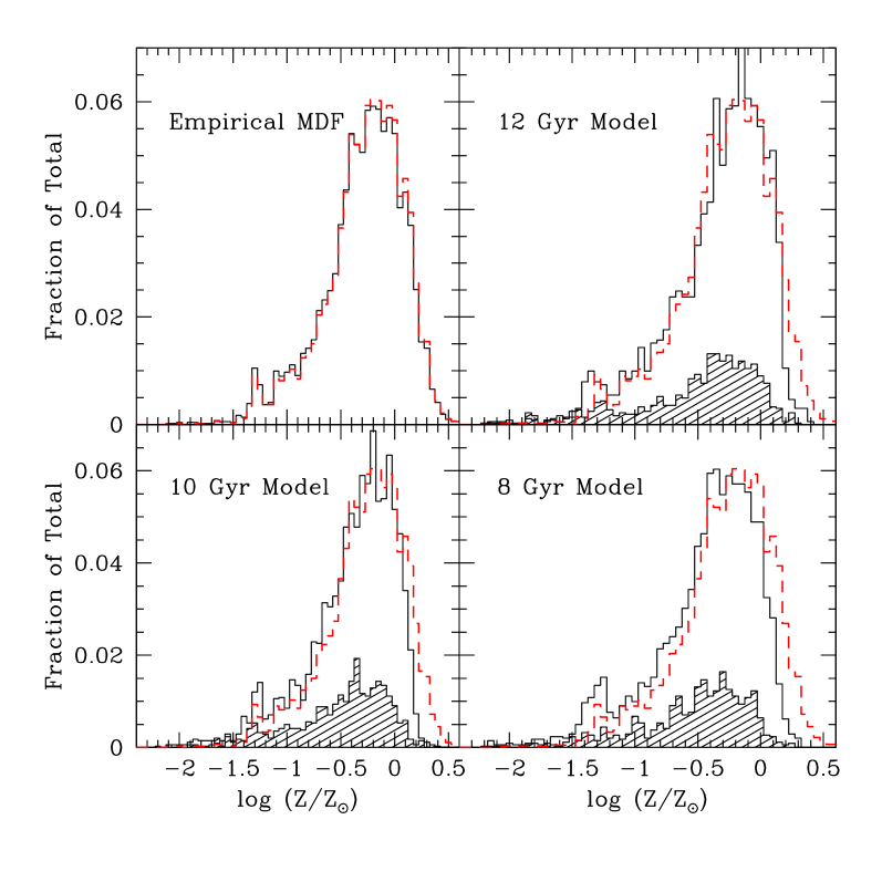
Figure 1: Upper left panel: Differential metallicity distribution function (MDF), normalized by the total number of stars, derived from the observed CMD through the interpolation on the grid of Teramo alpha-enhanced isochrones is shown with solid (black) line. The observed MDF including the correction for the AGB bias is overplotted as dashed red histogram. The other three panels show the MDFs from single burst simulations, where simulations had in input the observed (upper left black histogram) MDF and single age bursts of 8, 10, and 12 Gyr. The shaded histograms show the contribution of AGB stars as a function of metallicity, while the open histograms show the contribution of only the RGB stars for each simulation. The MDFs of these simulated data are constructed in exactly the same way as for the observations, by interpolating over the isochrones in CMDs after the photometric errors were added to the simulated stars, and can therefore be compared directly with the observed AGB bias corrected MDF, which is overplotted with red dashed histogram.

The bolometric corrections in this work are taken from Girardi et al. (2002), while in Paper I we used the tables of Zoccali et al. (2003), based on the empirically determined BCs (Montegriffo et al. 1998). The main difference between the two is in regard to the treatment of the red giants with colours $V-I\ga 3.6$, equivalent to temperatures below $\sim 3250$ K, for which the Montegriffo et al. (1998) bolometric corrections are several magnitudes larger (in absolute value) than those of Girardi et al. (2002). For giants with temperatures between $\sim 3800-3250$ K ($1.8\la V-I\la 3.6$) the difference between the two scales is up to 0.5 mag; in this temperature range the Montegriffo et al. (1998) bolometric corrections are actually smaller in absolute value, while for the hotter giants the two scales match very well. For the derivation of the empirical MDF from the observations the bolometric corrections were calibrated on Galactic globular clusters, as described in Harris & Harris (2000).

The MDF we used in input for the simulations has been carefully derived. In particular we introduce a correction to the empirical first-order MDF, to remove what we will call the AGB bias. The grid of isochrones we use to determine the empirical MDF consists of the evolutionary tracks for the RGB stars, i.e. those along the first ascent of the giant branch. However, in any real sample of stars, AGB stars (second ascent of the giant branch) are also present, and these are slightly bluer than the RGB at a given metallicity and luminosity. Thus the empirical MDF derived from all the stars will end up slightly biased to lower metallicity than it should. In addition, because our data contain a wide range of metallicities, the AGB and RGB populations are heavily overlapped and we cannot remove the AGB bias just by cutting off the bluest end. However, the simulated CMDs contain all the information we need about the evolutionary stages of the stars in any given region of the CMD, so we use these to find out what fraction of the total population belongs to the AGB, and how they are distributed in metallicity.

We first create the synthetic CMDs for single age populations with 8, 10 and 12 Gyr isochrones and the input “empirical MDF” derived from the interpolation of colours of all stars with magnitudes between $-3.6<M_{bol}<-1.4$ in the observed CMD. In these synthetic CMDs we selected only the first ascent giants (RGB stars) and re-derived the new MDF in the same way as for the observations: interpolating the RGB stars colours with $-3.6<M_{bol}<-1.4$ on the same set of models. This new MDF is the so-called AGB bias corrected MDF. In the same way we also derive the MDF for only AGB stars for each simulation. In Fig. 1 we compare the differential MDF histogram derived from observations (upper left) with MDFs from three single age simulations run with empirical observed MDF in input and ages of 8, 10, and 12 Gyr. In all cases MDFs were constructed with stars in the range $-3.6<M_{bol}<-1.4$ and are normalized by the total number of stars. The shaded histograms show the MDFs of AGB stars, while the open histograms show the MDFs of only the RGB stars in the given simulation. For comparison in each diagram we also overplot the empirical observed MDF including the AGB bias correction as a red dashed histogram, renormalized to the same total number of stars. As can be seen from the upper left panel of Fig. 1, the AGB bias correction turns out to have quite a small systematic effect on our empirical MDF, with the main correction being the reduction of the already-small metal-poor tail.

Evaluation of our models in the $8-12$ Gyr range shows that over the luminosity range $-3.6<M_{bol}<-1.4$ that we use to determine the MDF, the RGB stars contribute 76% of the total population, with the rest being the AGB contaminants. The actual ratio depends weakly on metallicity itself, but is well represented by a simple interpolation curve that we obtain from the simulations,

$$\frac{N_{RGB}}{N_{total}}=0.098{\rm[Z/H]}+0.816\,.$$ (1)

This curve accurately represents the ratio to within $\pm 0.05$ at any metallicity and any age within the stated range; the scatter about this mean line is produced mainly by the bin-to-bin Poisson fluctuations in the sample sizes that we are working with. Thus at the extreme metal-poor end the AGB stars make up almost 40% of the population, falling to $\sim 20$% at solar metallicity and above. Because the metal-poor bins in our observations contribute only small numbers of stars, the global average of $\mathrm{N}_{RGB}/\mathrm{N}_{total}=0.78$ is dominated by the heavily populated metal-richer bins.

Fig. 1 also shows the classic age-metallicity degeneracy. The 12 Gyr model matches the empirical MDF used in input closely, as expected because 12 Gyr isochrones are used to determine the MDF. For successively younger ages (most noticeable for the 8 Gyr model), the deduced MDF maintains the same shape but shifts slowly to more metal-poor values, at the rate of about 0.1 dex per 3-4 Gyr. In Paper I, we found the same amount of shift when using the Victoria isochrones (VandenBerg et al. 2000). In short, from the RGB stars alone, we cannot tell the difference between a 12 Gyr population with the input MDF, and a population that is a few Gyr younger and intrinsically more metal-rich by 0.1-0.2 dex in the mean. The most important way we have to break this degeneracy is to use the colour distribution and luminosity function of the RC, as we show later.

The observed empirical MDF, and the resulting MDF corrected for the AGB bias, are given in Table 1. In the rest of the paper, when we refer to “input observed” cumulative MDF, we mean this bias corrected MDF (third column of Table 1).

Table 1: Observed metallicity distribution function for stars in the halo field of NGC 5128. The second column lists the total number of stars in each metallicity bin, while the third column gives the number of first ascent red giants in each metallicity bin, after the correction for the AGB contribution.

$\log(Z/Z_{\odot})$	N	NRGB	$\log(Z/Z_{\odot})$	N	NRGB
-2.05	0	0	-0.65	101	76.0
-1.95	3	1.9	-0.55	122	93.0
-1.85	1	0.6	-0.45	188	145.1
-1.75	1	0.6	-0.35	194	151.6
-1.65	2	1.3	-0.25	247	195.5
-1.55	3	2.0	-0.15	237	189.9
-1.45	10	6.7	-0.05	225	182.5
-1.35	37	25.3	0.05	218	179.0
-1.25	23	16.0	0.15	111	92.2
-1.15	38	26.7	0.25	35	29.4
-1.05	48	34.2	0.35	8	6.8
-0.95	46	33.3	0.45	1	0.9
-0.85	59	43.2	0.55	3	2.6
-0.75	97	72.0	0.65	0	0

As in Paper I we adopt E(B-V)=0.11, the Cardelli et al. (1989) extinction law, and the distance modulus of $(m-M)_{0}=27.92$ (Rejkuba 2004; Harris et al. 2010). All simulations are derived with a single slope IMF with $\alpha=2.35$ (Salpeter 1955), and masses $0.5<M/M_{\odot}<3$. Furthermore the simulations include the correct photometric errors and completeness as derived from the artificial star experiments in Paper 1. These parameters are kept constant throughout. What we change are the evolutionary background (solar scaled, alpha enhanced models), the age, and the metallicity distribution.

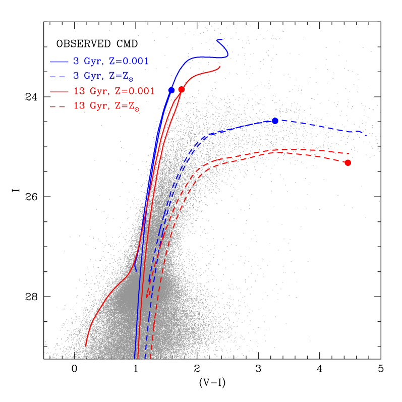
Figure 2: Observed CMD with 3 (blue) and 13 Gyr (red) isochrones overplotted. Dashed lines are used for solar (Z=0.0198) isochrones, while solid lines show metal-poor (Z=0.001) isochrones.

The final set of single age simulations that we use to compare with the observations includes:

1. single age burst models with input observed MDF and ages ranging from 2 to 13 Gyr, with a step size of 0.5 Gyr; These simulations were run until the number of stars in a box on the upper RGB ($24.5<I<26$ and $1.0<V-I<2.3$) matched the observed $N_{box}=3131$ stars (Sect. 4.1).

2. single age burst models with a MDF following the closed box model with a range of yields, and minimum/maximum metallicities. As for the previous case the number of stars in the same box on the upper RGB was used as the condition to stop the simulation (Sect. 4.3).

3. single age burst models with a flat MDF selecting different metallicity ranges. These simulations had as a stopping condition 50,000 output stars (stars that passed all observational tests).

The simulations with either the input observed MDF or a closed box MDF were compared directly with the observed CMD. The set of isochrones used to generate simulated CMDs includes the following metallicities: Z=0.0001, 0.0003, 0.0006, 0.001, 0.002, 0.004, 0.008, 0.01, 0.0198 (solar), 0.03, and 0.04.

Going beyond these single-age models, we next used these as input to construct more complex (multi-burst) star formation histories. In particular single age flat MDF simulations were used to explore some complex star formation histories with specific age-metallicity relation. We did not include the simulations having single metallicity and age distribution, because the observed RGB is far too wide to be reproduced in this way. The colour distribution on the bright RGB is far more sensitive to metallicity than it is to age, compared with other parts of the observed CMD. Therefore we use it as our primary metallicity indicator.

As will be seen in the next sections, the basic direction in which our conclusions are heading is that the NGC 5128 halo stars are predominantly old and with a very wide metallicity range. We illustrate the essential idea in Figure 2, where the observed CMD is overplotted with isochrones for low Z (Z=0.001) populations of two ages that cover the range we will be interested in (3 and 13 Gyr), and also solar metallicity ($Z_{\odot}=0.0198$) isochrones of the same two ages. A wide range of ages at any single metallicity cannot accommodate the wide observed range of colours; the low metallicity isochrones are too blue for any age and the high metallicity isochrones are too red. Moreover, the young, 3 Gyr old isochrones overshoot the upper envelope of the observed RGB by about 1 mag: such a young component, if present, must involve a very modest amount of stellar mass to match the lack of stars brighter than the RGB tip. In addition, NGC 5128 must contain a large component that is both old and very metal-rich, because many RGB stars are redder than the young (3 Gyr) solar isochrone.

Finally, the model is matched to the observed CMD by dividing the colour/magnitude plane into a grid, comparing the number of real and model stars in each cell of the grid, and calculating the $\chi^{2}$ goodness of fit between the two. Other diagnostics, such as luminosity function fits and ratios of stars in different evolutionary phases, are used as well to decide on the best result. We first describe in detail our choice of full CMD fitting, and then give some details about other diagnostic diagrams, before launching into the discussion of the results of our experiment.

Appendices A and B (published only in the electronic form) list all single age simulations we explored as well as double burst simulations that were compared with the observations. All the single age simulations that are made using solar scaled isochrones have names starting with ”sol*” and those that have alpha enhanced models are named ”aen*”. All combined simulations have names starting with ”cmb*”.

3.2 Approach to matching the full CMD

In previous studies, opinions have varied about how best to perform the matchup between the observed and simulated CMDs. For example, Harris & Zaritsky (2001); Aparicio & Hidalgo (2009) and others have used a $\chi^{2}-$minimization criterion across the grid to find the best range of input-model parameter space. On the other hand, Dolphin (2002) strongly advocates the use of a cumulative likelihood ratio, arguing that the number counts within the grid cells intrinsically follow the Poisson distribution rather than the Gaussian statistical rules that are implicit in a $\chi^{2}$ calculation. We would agree with Dolphin’s precepts in the limit where the number $n$ of objects per cell is small, e.g. $n\lesssim 10$. Such a limit would apply for cases in which many of the regions in the CMD that are of key interest are very sparsely populated, even when the total population $N$ is large and the cell size is comparable with the size of the measurement errors in magnitude and colour. However, that situation is not the case for our data since, for our grid definition, $n$ is always larger than 200. In the limit of large $n$ the Poisson distribution converges smoothly to the Gaussian one, and the practical difference between the $\chi^{2}$ statistic and the likelihood ratio is moot (see also Brown et al. 2006; Tolstoy et al. 2009, for direct comparisons and a similar conclusion).

Another initial choice for the numerical setup is how to lay out the grid cells. We have experimented with a uniform grid (all cells the same size in both coordinates) and also with an “adaptive grid” (Harris & Zaritsky 2001; Aparicio & Hidalgo 2009) where the cells are smaller in areas of higher stellar density, and where the stellar evolutionary models are more accurate and precise. Based on similar experiments Harris & Zaritsky, find that the best-fit solutions are relatively insensitive to the particular grid structure. We have found the same basic effect. For the final runs we adopt an adaptive grid (see below) in which the number $n$ per cell remains very roughly constant, though it is still fine enough to track the most important changes in the stellar distribution with age and metallicity. Dolphin (2002) suggests that the bin size should be comparable to the size of the smallest features in the CMD to which we want to be sensitive. In practice, however, this criterion can be compromised by the photometric measurement scatter and incompleteness, which (especially at the faint end) set a lower limit to the cell size that will be physically meaningful. Smaller differences in the stellar distribution will be blurred out even if they resulted from important differences in the age/metallicity history that we might have hoped to measure. Therefore, in our grid the minimum cell size is similar to the observational uncertainties in magnitude and colour.

Table 2: Adopted grid for the computation of the $\chi^{2}$ for the full CMD fit. Magnitudes and colours are given in the observed plane, without extinction correction. Column 6 lists the weight, column 7 gives the number of stars in the observed CMD.

(1)	(2)	(3)	(4)	(5)	(6)	(7)	(8)
#	$I_{1}$	$I_{2}$	$(V-I)_{1}$	$(V-I)_{2}$	$w$	$N_{obs}$	Comment
1	28.40	28.80	-0.25	0.55	0.3	781	at 50% completeness edge; $\sigma_{I}$=0.25-0.3, $\sigma_{V}=0.15-0.2$
2	28.40	28.80	0.55	0.90	0.4	2027	partly below 50% line; $\sigma_{I}=0.25-0.3$, $\sigma_{V}=0.2-0.25$
3	28.40	28.80	0.90	1.35	0.2	1508	partly below 50% line; $\sigma_{I}=0.25-0.3$, $\sigma_{V}=0.2-0.25$
4	28.05	28.40	0.15	0.70	0.8	1145	$\sigma_{I}=0.2-0.25$, $\sigma_{V}=0.2$
5	28.05	28.40	0.70	0.90	0.8	2111	$\sigma_{I}=0.2-0.25$, $\sigma_{V}=0.2$
6	28.05	28.40	0.90	1.10	0.6	2894	close to 50% line; $\sigma_{I}=0.2-0.25$, $\sigma_{V}=0.25$
7	28.05	28.40	1.10	1.35	0.5	2854	close to 50% line; $\sigma_{I}=0.2-0.25$, $\sigma_{V}=0.25$
8	28.05	28.40	1.35	1.65	0.4	639	partly below 50% line; $\sigma_{I}=0.2-0.25$, $\sigma_{V}=0.3$
9	27.70	28.05	0.30	0.70	0.4	418	some scattered/foreground stars?
10	27.70	28.05	0.70	0.90	1.0	2212	$2\sigma$ off in color from the RC
11	27.70	28.05	0.90	1.01	1.0	2750	RED CLUMP MAXIMUM $\sigma_{I}=0.18$, $\sigma_{(V-I)}=0.2$
12	27.70	28.05	1.01	1.24	1.0	7351	RED CLUMP MAXIMUM $\sigma_{I}=0.18$, $\sigma_{(V-I)}=0.2$
13	27.70	28.05	1.24	1.36	1.0	2775	RED CLUMP MAXIMUM $\sigma_{I}=0.18$, $\sigma_{(V-I)}=0.2$
14	27.70	28.05	1.36	1.59	1.0	2399	$2\sigma$ in color off from the RC
15	27.70	28.05	1.59	1.90	0.4	444	at the 50% limit
16	27.40	27.70	0.40	0.93	0.8	633	$\sigma_{I}=0.15$, $\sigma_{V}=0.1$
17	27.40	27.70	0.93	1.13	1.0	2039	$1-3\sigma$ above the RED CLUMP
18	27.40	27.70	1.13	1.28	1.0	2077	$1-3\sigma$ above the RED CLUMP
19	27.40	27.70	1.28	1.48	1.0	1624	$1-3\sigma$ above the RED CLUMP
20	27.40	27.70	1.48	2.00	0.8	631	$\sigma_{I}=0.15$, $\sigma_{V}=0.2$ (lower weight due to larger V error)
21	27.20	27.40	0.55	1.02	0.9	299
22	27.20	27.40	1.02	1.18	1.0	627
23	27.20	27.40	1.18	1.33	1.0	747	$\sigma_{I}=0.1$, $\sigma_{V}=0.1$
24	27.20	27.40	1.33	1.48	1.0	414
25	27.20	27.40	1.48	1.95	0.9	255
26	27.00	27.20	0.60	1.10	1.0	291
27	27.00	27.20	1.10	1.25	1.0	489
28	27.00	27.20	1.25	1.40	1.0	487
29	27.00	27.20	1.40	1.92	1.0	392
30	26.85	27.00	0.70	1.15	0.9	258
31	26.85	27.00	1.15	1.30	1.0	458
32	26.85	27.00	1.30	1.45	1.0	458
33	26.85	27.00	1.45	1.90	0.9	262
34	26.70	26.85	0.75	1.18	1.0	268
35	26.70	26.85	1.18	1.26	1.0	241	within $1.5\sigma$ from AGB bump
36	26.70	26.85	1.26	1.35	1.0	333	AGB BUMP PEAK $\sigma_{I},\sigma_{(V-I)}=0.085$
37	26.70	26.85	1.35	1.46	1.0	336	within $1.5\sigma$ from AGB bump
38	26.70	26.85	1.46	1.90	1.0	327
39	26.55	26.70	0.85	1.25	1.0	337
40	26.55	26.70	1.25	1.43	1.0	508	$2\sigma$ from AGB bump in magnitude
41	26.55	26.70	1.43	1.92	1.0	367
42	26.30	26.55	0.90	1.25	1.0	305
43	26.30	26.55	1.25	1.40	1.0	522
44	26.30	26.55	1.40	1.55	1.0	433
45	26.30	26.55	1.55	2.00	1.0	306
46	26.00	26.30	0.95	1.30	1.0	276
47	26.00	26.30	1.30	1.45	1.0	432
48	26.00	26.30	1.45	1.60	1.0	383
49	26.00	26.30	1.60	2.10	1.0	375
50	25.60	26.00	1.05	1.40	1.0	309
51	25.60	26.00	1.40	1.55	1.0	387
52	25.60	26.00	1.55	1.80	1.0	420
53	25.60	26.00	1.80	2.50	1.0	314
54	25.00	25.60	1.10	1.50	1.0	325
55	25.00	25.60	1.50	1.75	1.0	413
56	25.00	25.60	1.75	2.10	1.0	359
57	25.00	25.60	2.10	3.00	1.0	338
58	23.80	25.00	1.25	1.85	1.0	338
59	23.90	25.00	1.85	2.40	1.0	406
60	24.00	25.00	2.40	3.00	1.0	300
61	24.25	25.60	3.00	4.50	0.8	380	lower weight due to uncertain bolometric corrections for cool RGB stars

Beyond these numerical criteria, our approach to matching the model and observed CMDs is more strongly driven by the astrophysical limitations of our data than by statistical formalism. Most previous studies of this type (Aparicio et al. 1997; Dolphin 2002; Harris & Zaritsky 2004; Brown et al. 2006; McQuinn et al. 2009; Vanhollebeke et al. 2009, among others), including such targets as the Galactic bulge, the Magellanic Cloud field-star populations, the M31 outer disk, and nearby dwarf galaxies, employ CMD data that cover a wide luminosity range from the tip of the RGB down to below the turnoff point of the classic old population, giving the strongest possible leverage on the age distribution independently of metallicity. These target fields also typically include stars over wide ranges of both age and metallicity, with very significant young components.

By contrast, the NGC 5128 halo stars cover a relatively small range in age (with only a small and perhaps negligible fraction younger than $\sim 5$ Gy) but a very large range in metallicity (see Paper I). In addition, we have only the luminosity range of the HB and above to work with. This more restricted range in the evolutionary stages of the stars can still yield solutions for the age distribution that are accurate (that is, they return systematically correct age ranges), though they are very definitely less precise (that is, with larger uncertainties) than if the turnoff region were included; see, for example, the simulation tests in Dolphin (2002), particularly his Fig. 7 and accompanying text.

The size of our dataset of $\sim 70,000$ stars (less than 56,000 are above 50% completeness limit and only these are compared to the models) is smaller than samples studied for example by Harris & Zaritsky (2001, 2004), who observed $4\times 10^{6}$ LMC field stars and $6\times 10^{6}$ stars in the SMC, as well as the sample of Vanhollebeke et al. (2009), who had $6\times 10^{6}$ stars in their Galactic-bulge study, and of Brown et al. (2006), who had $\sim 10^{6}$ stars in their study of the M31 disk and halo. It resembles more closely instead the sample sizes of the Fornax dSph (Coleman & de Jong 2008), the nearby starburst dwarfs studied by McQuinn et al. (2009), and the M81 outer-disk and dwarf satellite studies of Weisz et al. (2008) and Williams et al. (2009). We note however that the targets from the above mentioned studies exhibit either well sampled main sequences or in some cases very obvious young components, hence providing evidence of a wide total age mixtures unlike our pure old-halo sample.

Thus, within the limitations of the present data we can ultimately determine only some appropriate ranges for the age distribution and the star formation history. The model fits to be discussed below are definitely capable of ruling out large sections of the total parameter space. But the classic age/metallicity/alpha-enhancement degeneracies that affect the high-luminosity regions of the CMD for extremely old stellar populations leave us unable to isolate a single “best” solution. Nevertheless, some clear conclusions emerge about such important features as the minimum age spread and the relative proportions of stars in different age ranges, that go well beyond our initial study in Paper I.

3.3 Diagnostics

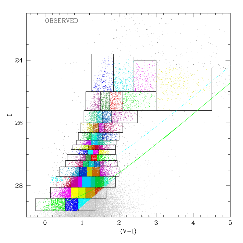
Figure 3: Observed CMD with overplotted “adaptive grid” based on which $\chi^{2}$ of the CMD fit is computed.

Before going into the results of the modeling, we describe here the diagnostics used to evaluate the goodness of the fit between the various models and the observations.

1. Comparison of the luminosity functions in V and I:

   We check the positions of maxima of the RC and AGB bump features, the width of these features, and the $\chi^{2}$ fit over the whole LF. This comparison is done only for magnitudes above the 50% completeness limits: $V<29.65$, and $I<28.8$.

2. Comparison with overall $\chi^{2}$ of the CMD:

   The $\chi^{2}$ is calculated with the following formula:

   $$\chi^{2}=\frac{\Sigma_{i}(N_{obs,i}-N_{sim,i})^{2}*w_{i}}{N_{obs,i}}$$ (2)

   where $N_{obs,i}$ is the number of observed stars in the $i-th$ box, $N_{sim,i}$ is the number of simulated stars in the $i-th$ box, and $w_{i}$ are the weights (normalized to have the sum of 1). The reduced $\chi_{\nu}^{2}$ is given by the ratio of $\chi^{2}$ to the number of boxes.

   The boxes are shown in Figure 3, and are listed in Table 2. They have been chosen based on features in the observed CMD, combined with the photometric accuracy, completeness and uncertainty in the bolometric corrections. In particular, we selected larger box sizes in the faint part of the CMD to accommodate for the scattering of stars due to photometric errors. The boxes in the middle of the CMD where the number of stars is large are small in colour-magnitude space, but get wider at the edges of the RGB, in order to maintain the statistics. In the upper part of the diagram the boxes are very large to sample at least 250 stars, and the reddest box is wide enough to cope with the changing shape of the simulated extent of the cool red giant branch possibly due to inaccuracies in the colour-temperature transformations.

   We also tested our results using the regular grid with smaller boxes over the CMD, but excluding the reddest part of the RGB ($V-I>2.4$). While the values of the reduced $\chi_{\nu}^{2}$ turn out to be sensitive to the grid size and number of cells, the indication as to the best fitting models was robust.

   To check the sensitivity of the $\chi^{2}$ tests, we run several simulations with different random seeds in input and then compared those with other simulations with the same set of parameters. This then allows us to estimate an error on $\chi^{2}$ values due to simple Poissonian statistics (since the sample of the observed/simulated stars is limited). The systematics can be assessed better by comparing simulations vs. simulations while changing one of the parameters (see discussion below and Figure 4).

3. Comparison with stellar counts on the RC and AGB bump:

   This diagnostic is based on selected boxes along the RGB that target features sensitive to age and metallicity distribution, like the RC and the AGB bump. The stellar counts for the RC are assumed to be the sum of all stars in the boxes 11, 12 and 13 indicated as RC maximum boxes in Table 2 and covering the range $27.7<I<28.05$ and $0.9<V-I<1.36$. The total number of stars in the observed CMD within these boxes is 12876. The stellar counts for the AGB bump feature are constructed by summing all stars within boxes 31, 32, 35, 36, 37 and 40 (Table 2) that cover the range between $26.55<I<26.7$ and $1.15<V-I<1.46$ which is within $2\sigma$ of the AGB bump magnitude and colour peak. The total number of stars in the observed CMD within these boxes is 2334.

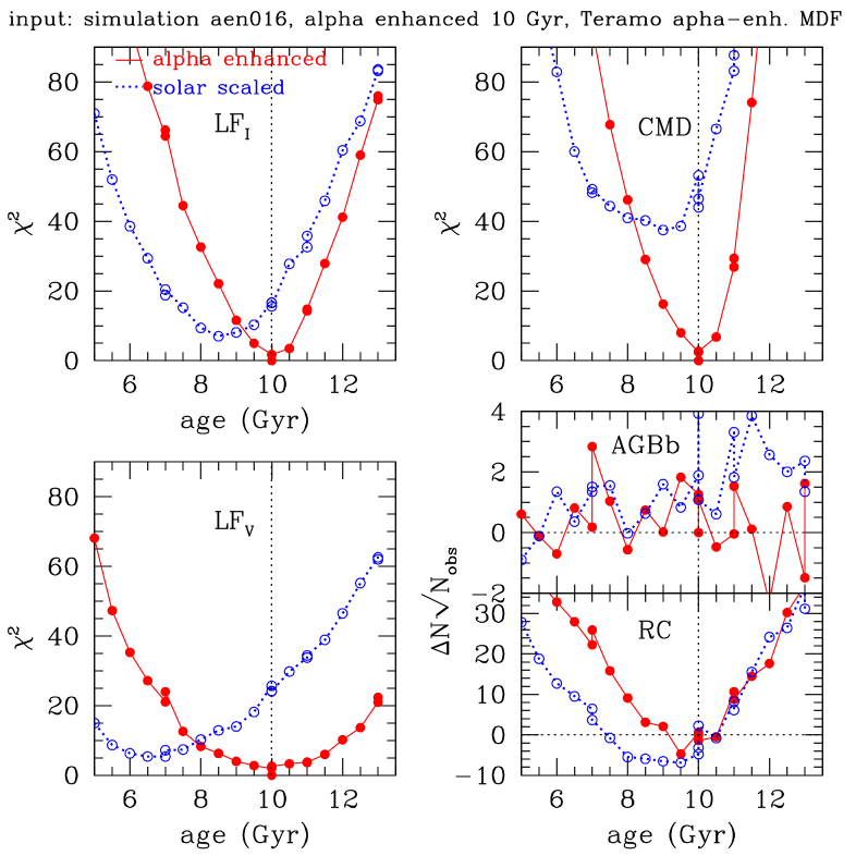
Figure 4: Comparing a single burst simulation for 10 Gyr old burst with alpha enhanced stars against all single age simulations as a test of the diagnostics. On the left are $\chi^{2}$ diagnostics based on the I-band LF (upper left) and V-band LF (lower left). The upper right panel shows the diagnostic power of the full CMD fitting, while the lower right panel compares the number of red clump (RC) and AGB bump stars as a function of age. $\Delta N$ is the difference between the number of stars in the “input” (in this case simulation aen016) and the number of stars in the same boxes in the simulated CMD, normalized to the Poissonian noise of the number of “observed” (input) stars. Simulations constructed with $\alpha$-enhanced isochrones are shown with red filled dots, and solar scaled models are plotted with blue open symbols.

To gauge the sensitivity of our diagnostics on the age we show in Figure 4 the results of a comparison between a set of single age simulations using a template simulation (aen016) constructed with alpha-enhanced 10 Gyr old models and the input observed MDF. The four panels refer to different diagnostics, namely the $\chi^{2}$ fit of the luminosity functions in the $V$ and $I$ bands, and of the overall CMD, and the number of stars in the Red Clump and AGB bump. The various models assume the same input MDF as the template simulation and the models shown in red (filled dots) assume alpha enhanced isochrones with various ages. The $\chi^{2}$ value of the fit for the red model with an age of 10 Gyr with respect to the template simulation is 1, as expected when comparing two simulations with all input parameters the same, except the difference in the initial random number seed. The blue dotted curves (and open circles), instead, refer to models based on the solar scaled isochrones of the BASTI set, and are meant to explore what happens if we use solar scaled tracks to interpret alpha enhanced stars. The pronounced minima in the $\chi^{2}$ curves show that (in this very basic comparison) the diagnostic on the age is good. Different $\chi^{2}$ diagnostics show that full CMD fitting and the I-band LF are the most sensitive. When using solar scaled isochrones, the LFs yield an age systematically too young, but the $\chi^{2}$ for the overall CMD clearly indicates the need for alpha-enhanced tracks to match the template simulation. The number of red-clump stars is also a fair age indicator, with the appropriate (alpha enhanced) isochrones, though we note that the sensitivity of this indicator is somewhat lower than for the full LF and CMD fits.

The population size in the AGB bump, instead, is not very sensitive to age. This is certainly in part due to the smaller overall number of stars in the AGB boxes, combined with the internal photometric scatter. Therefore the total number of stars is a less useful diagnostic, than is the position (luminosity and colour) of the AGB bump.

The real sensitivity of our diagnostics will certainly be worse than what is described so far, since observations differ from the template simulation in many respects, e.g. in the age spread. In the next section we compare the data and simulations.

4 Results

In this section we take the approach of exploring the range of acceptable ages and age distributions for the observed CMD. First we compare with the single-age simulations and show that a single-age burst cannot fully reproduce the observations. Next, we show that some two burst simulations fit the observations equally well in terms of overall CMD fit, but significantly better when comparing the luminosity functions. Finally, we explore some simple solutions with multi-age and multi-enrichment components. In principle by adding additional free parameters (percentage of stars of a given age and metallicity with respect to the total population), it should be possible to find some “best fit” model(s). In practice the $\chi^{2}$ values for the full CMD fit do not go below $\sim 50$ likely due to the age-metallicity degeneracy in our observational dataset and the possibly inadequate combination of abundance ratios in the isochrones (see Figure 4). As stated earlier, the fact that the CMD does not reach the much more age-sensitive main sequence turnoff region limits the interpretation. We show only some selected plausible star formation histories that provide as good a fit to the observations as at least the best fitting double burst model does.

In addition to the comparison of the observed CMD with synthetic CMDs made with input observed MDF, we also explore alternative, physically motivated closed box chemical enrichment models.

4.1 Single age models with observed MDF

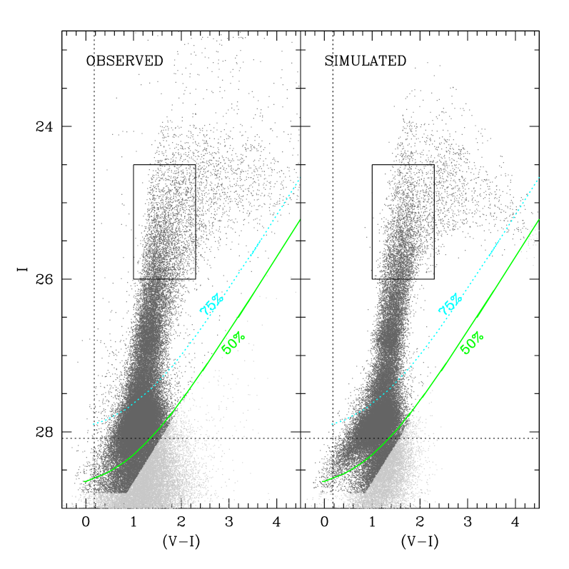
Figure 5: Left panel shows the observed and the right panel the simulated CMD for a single age burst population of 11 Gyr with the input observed MDF. The simulation uses alpha enhanced stellar evolutionary models.

In the right panel of Figure 5 we show the simulated CMD for a single age burst population of 11 Gyr with the input observed MDF made using the alpha enhanced isochrones. The number of stars in this simulation (and other single age + MDF simulations) was constrained to match the star counts in the box shown in the figure ($24.5<I<26$, $1.0<V-I<2.3$). This box contains 3131 stars and was chosen from the part of the CMD that is least sensitive to age, with the best photometric accuracy, and smaller uncertainty in the colour-temperature transformations.

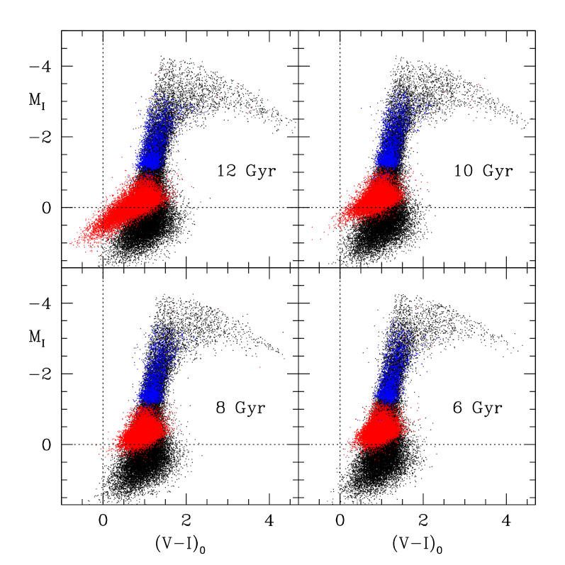
Figure 6: Simulations of CMDs with input observed MDF and single age burst using alpha enhanced stellar evolutionary models.

In the left panel of Figure 5 is the observed CMD. The overall appearance of the simulated CMD is fairly similar to the data; however some discrepancies are evident. Note the difference in the upper envelope slope for the RGB between models and observation: the simulations have a much stronger bend towards lower luminosity for the reddest red giants than is seen in the observed CMD. Possibly this is due to an overestimate of the bolometric correction (in absolute value) to the I-band magnitudes at low temperatures. We also notice that the RGB is narrower in the simulated diagram, likely indicating that a single age is not a good fit to the data. In the faintest part of the diagram the simulation shows more distinctly the core helium burning population, which in the data is more extended in colour, perhaps due to a combination of photometric errors and some age distribution effect. Finally, the red extension of the faintest portion of the diagram, below the 50% completeness line, is affected more by the uncertainty in photometric accuracy and completeness. Therefore we do not include that part (shown in light gray) in our fitting.

The widths of the RC and AGB bump features are smaller in the simulated CMD, also indicating that there may be a need to consider an extended star formation history.

In Figure 6 we show the sensitivity of the CMD to age. As expected, changes in the age make the most obvious differences in the RC feature; In this figure we colour-code the simulated stars according to their evolutionary status. In black we show first-ascent giants (RGB) stars, red shows core helium burners (RC) and in blue are the shell helium burners (AGB stars). It is clear that in the models with oldest ages ($>10$ Gyr) the blue tail of the core helium burning stars extends to much fainter magnitudes and bluer colours than in our data. The youngest model on the other hand has a brighter RC than does our observed CMD. These simulations, although simplistic, already suggest to us that the bulk of the stars in the NGC 5128 halo formed $\sim 10$ Gyr ago.

In the observed CMD within the RC region, the wide range of metallicities and the photometric measurement scatter make it impossible to say whether any particular star belongs to the RC or the RGB. Thus the RC colour difference with respect to the RGB colour at the same magnitude unfortunately cannot be used as an age discriminator (Hatzidimitriou 1991).

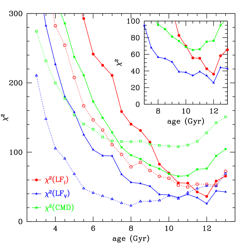
Figure 7: The $\chi^{2}$ diagnostic for luminosity function and full CMD fitting for observations with respect to all single age simulations. Comparison with the solar scaled single age simulations is shown with dotted lines (open symbols), and that with the alpha enhanced models with solid lines (solid symbols).

Figure 7 shows the $\chi^{2}$ diagnostic plots for observations with respect to all single age simulations. Each dot on this graph represents one single-burst model. These indicate that the dominant stellar population in the observed CMD is $11\pm 1$ Gyr old, and it appears to be more consistent with alpha enhanced abundance ratios. The solar scaled models produce CMDs that differ significantly more from the observed CMD, because they lack the stars along the blue edge of the RGB and RC. Notice that this applies also to the models constructed with the closed box metallicity distribution which has much more substantial population of low metallicity stars (Sect. 4.3).

Table 3: The three best fitting models for each diagnostic are listed for the single age simulations with input observed MDF. Diagnostics are $\chi^{2}$ for the full CMD, $\chi^{2}$ of the LF fit for I, and V-bands, and in the last two columns $\Delta N/\sqrt{N_{obs}}=\mathrm{N}_{obs}-\mathrm{N}_{sim}/\sqrt{N_{obs}}$ for the RC and AGBb boxes in our grid.

Single age models with input observed MDF
simulation	age	$\chi^{2}$	$\chi^{2}$	$\chi^{2}$	$\frac{\Delta N}{\sqrt{N_{obs}}}$	$\frac{\Delta N}{\sqrt{N_{obs}}}$
ID	(Gyr)	CMD	LFI	LFV	RC	AGBb
CMD:
aen025	10.5	65.2	55.7	34.5	-10.6	7.0
aen018	11.0	65.6	53.6	40.5	-0.9	8.8
aen024	11.0	66.2	55.3	39.1	1.1	7.4
LFI:
aen022	12.0	76.4	36.2	25.8	8.4	5.3
aen023	11.5	75.3	42.7	34.4	5.1	7.5
sol018	11.0	107.2	48.4	36.7	-3.7	9.1
LFV:
sol030	8.0	115.1	78.9	22.9	-15.8	7.4
aen022	12.0	76.4	36.2	25.8	8.4	5.3
sol031	7.5	115.4	96.7	26.6	-10.9	8.9
RC:
sol033	6.5	122.0	131.9	36.8	-0.1	7.8
aen030	8.0	95.7	140.4	56.5	-0.5	6.9
aen018	11.0	65.6	53.6	40.5	-0.9	8.8
AGBb:
aen022	12.0	76.4	36.2	25.8	8.4	5.3
aen020	13.0	104.4	65.5	42.8	28.6	6.1
sol040	3.0	274.4	426.2	210.5	48.1	6.1

Looking at individual diagnostics, the luminosity function $\chi^{2}$ fits for both I- and V-band point to an average single age of $12$ Gyr, while the overall CMD fit has a wider minimum at 10.5-11 Gyr. Table 7 (published in the electronic version) reports the $\chi^{2}$ values for all diagnostics, while the three best models for each individual diagnostic are reported in Table 3. From the inspection of this table it is evident that the counts in the RC region are consistent with $11$ Gyr model as well. We note however that this indicator is consistent also with the younger age of 8 Gyr, as found in Paper I. In these single age simulations AGB bump boxes are systematically less populated with respect to the observed CMD.

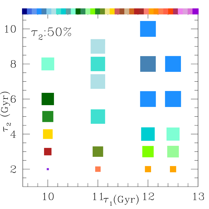
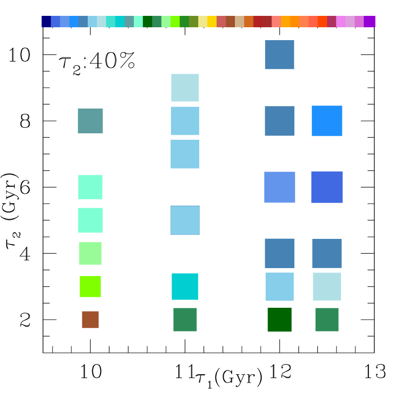
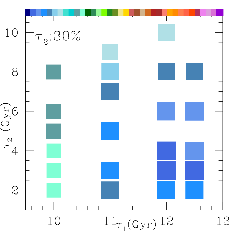
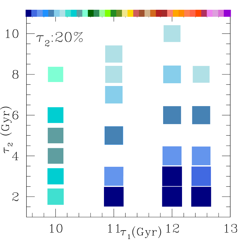
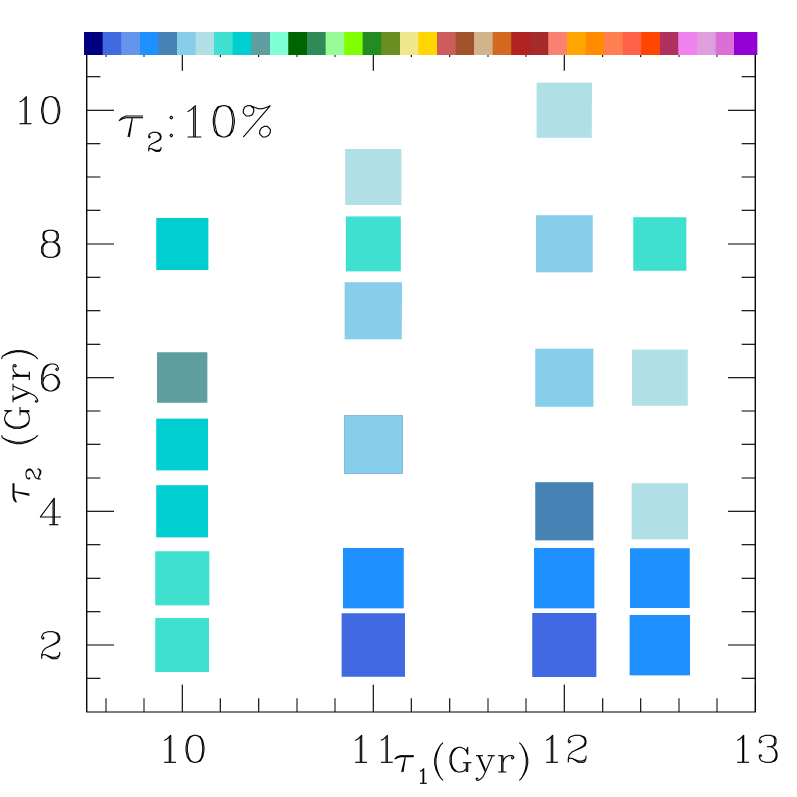
Figure 8: The $\chi^{2}$ diagnostic for the full CMD fit for 2 burst simulations, built using alpha-enhanced stellar evolutionary models, as compared to observations is plotted as a function of the old (x-axis) + young (y-axis) population age. Each panel shows different relative fractions of old + young population in the combined 2-burst simulation. The size and colour of the points are normalized to the full range of the $\chi^{2}$ values of the CMD fit for all 2-burst models with input observed MDF. The larger the symbol, and darker blue its colour, the smaller the $\chi^{2}$.

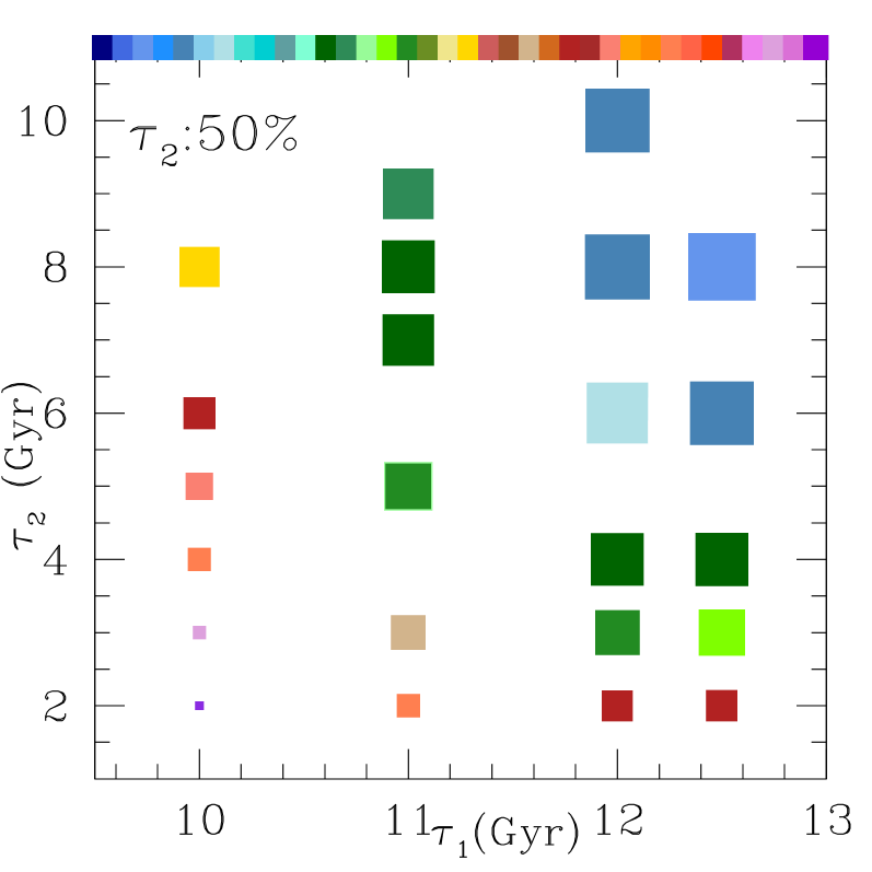
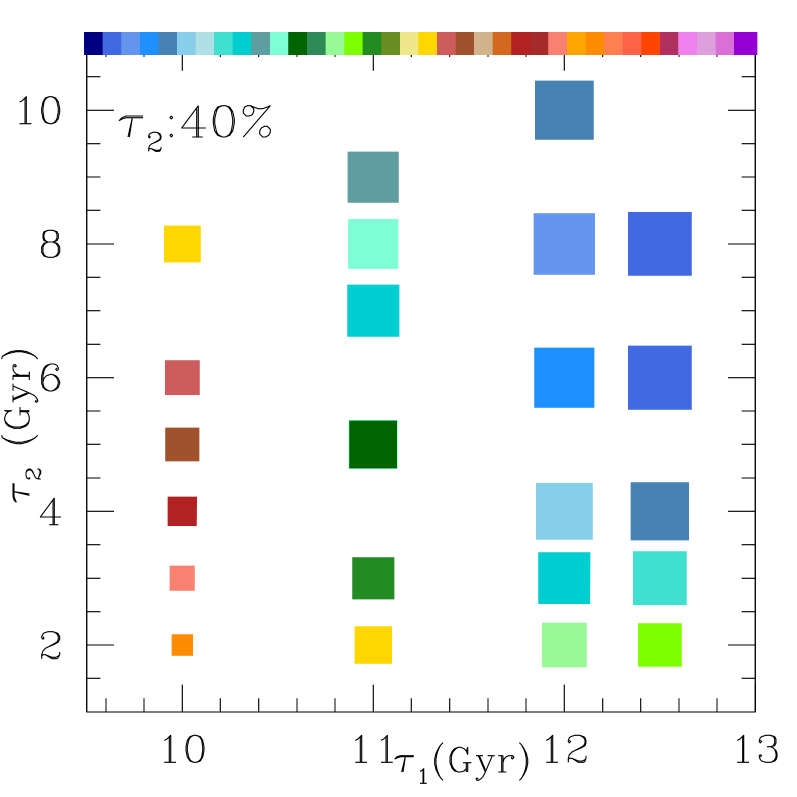
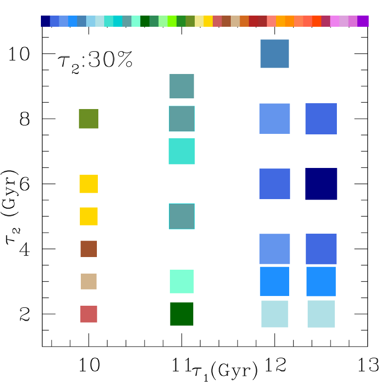
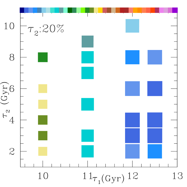
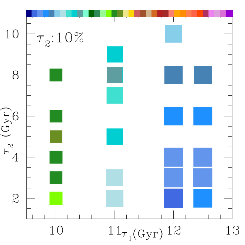
Figure 9: The $\chi^{2}$ diagnostic for the I-band LF fit for 2 burst simulations, built using alpha-enhanced stellar evolutionary models, as compared to observations is plotted as a function of the old (x-axis) + young (y-axis) population age. Each panel shows different relative fractions of old + young population in the combined 2-burst simulation. The size and colour of the points are normalized to the full range of the $\chi^{2}$ values of the LF_I fit for all 2-burst models with input observed MDF. The larger the symbol, and darker blue its colour, the smaller the $\chi^{2}$.

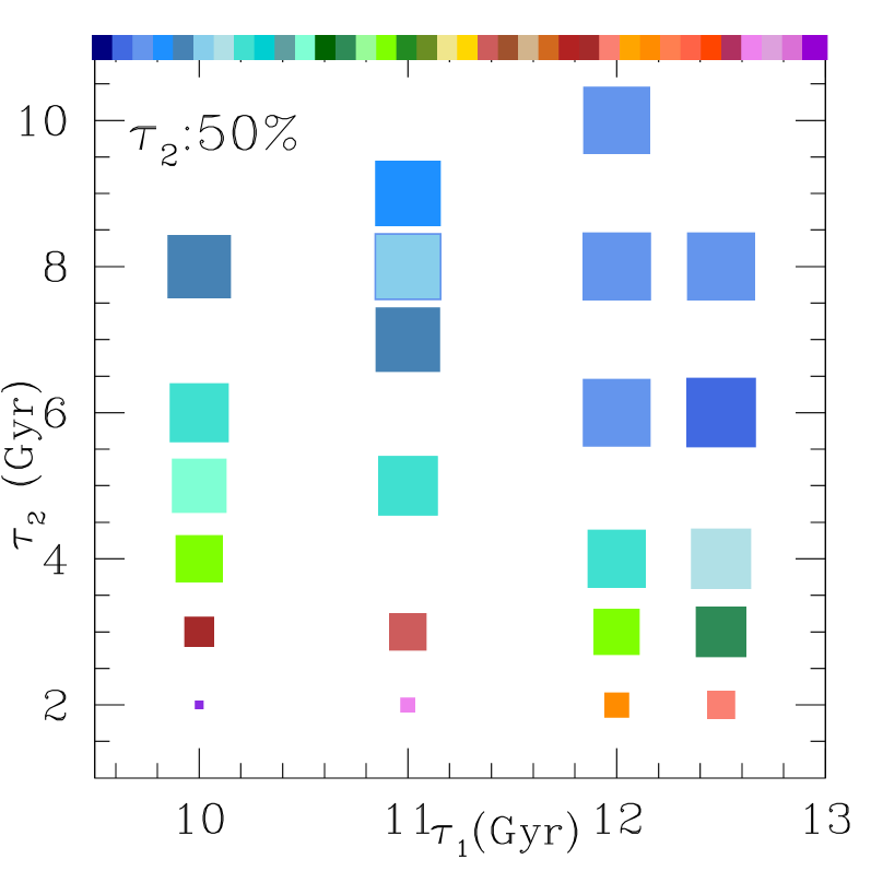
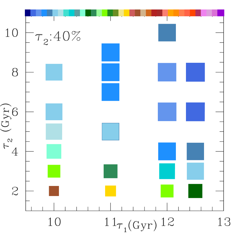
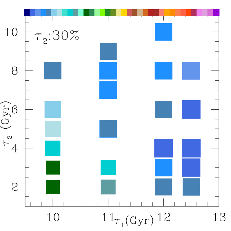
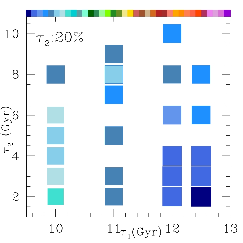
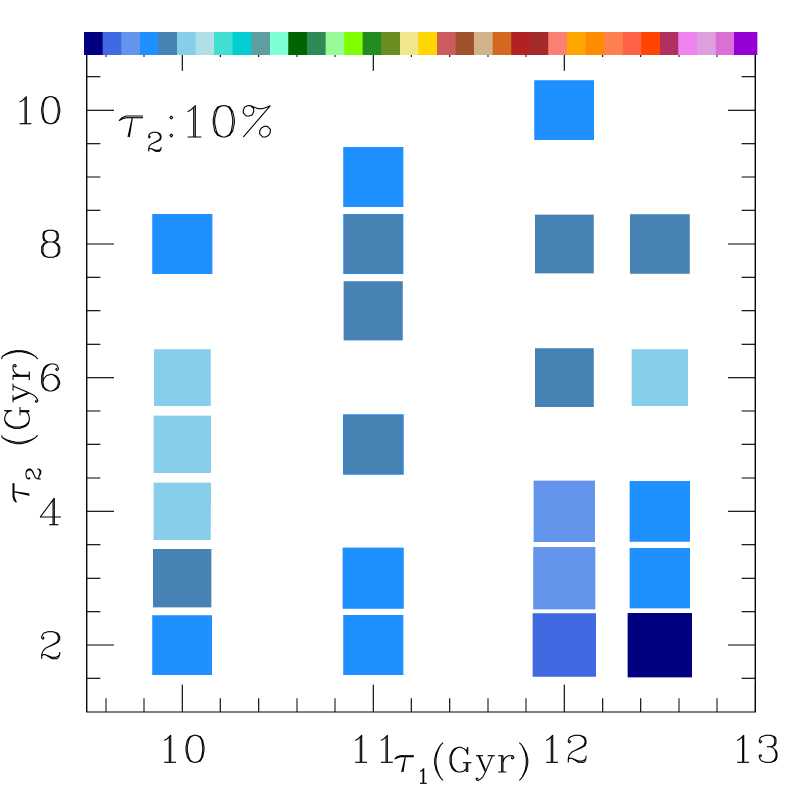
Figure 10: The $\chi^{2}$ diagnostic for the V-band LF fit for 2 burst simulations, built using alpha-enhanced stellar evolutionary models, as compared to observations is plotted as a function of the old (x-axis) + young (y-axis) population age. Each panel shows different relative fractions of old + young population in the combined 2-burst simulation. The size and colour of the points are normalized to the full range of the $\chi^{2}$ values of the LF_V fit for all 2-burst models with input observed MDF. The larger the symbol, and darker blue its colour, the smaller the $\chi^{2}$.

As already mentioned above, the single-age models produce widths of the RC and AGB bump features that are too narrow. In the next section we explore whether the fits are improved by adding a second age component, hence simulating a two bursts star formation history. This is motivated also from other observations: NGC 5128 is likely to have experienced a history of satellite accretions (minor mergers), but also some previous observations of resolved stellar populations and globular clusters have implied a smaller population of younger stars with ages close to $\sim 3-5$ Gyr (Soria et al. 1996; Marleau et al. 2000; Rejkuba et al. 2003; Woodley et al. 2010b).

4.2 Two burst simulations

A series of two burst simulations was created first by randomly drawing from an old single age simulation a certain percentage P1 of the total number of stars. Then, we add to the list a percentage P2 of a younger population, again drawing stars randomly from a single age simulation. By definition $P1+P2=100$%, and both components were given the input observed MDF. When drawing the stars randomly from the parent single age simulations, we verify that the final combined simulation has MDF bins populated such that it matches the observed MDF. Therefore, since the metal-poor bins have fewer stars, and since the old age (P1) simulation is first extracted, the metal-poor bins on average have an older age. We note however, that the combined CMD also contains some metal-rich stars from the old (P1) episode.

The combinations simulated in this way have relative percentages of 90-10, 80-20, 70-30, 60-40, and 50-50 old+young stars. The old component was allowed to range between 10.0 and 12.5 Gyr, and the young component between 2 and 10 Gyr. In addition to mixing alpha enhanced simulations (for both old and young age), we also considered that the younger population might have lower alpha enhancement, and thus we combined old alpha enhanced models with younger solar scaled simulations. Table 9, given fully in the electronic format, lists all 2-burst simulations we considered and it shows also the $\chi^{2}$ values for our fit diagnostics. Table 4 lists the best fitting models separately for each diagnostic. Here we summarize the main conclusions based on the inspection of these diagnostics and careful inspection of simulated CMDs.

Table 4: The best fitting models for each diagnostic are listed for the two burst combinations with the input observed MDF. Diagnostics are $\chi^{2}$ for the full CMD, $\chi^{2}$ of the LF fit for I, and V-bands, and in the last two columns $\Delta N/\sqrt{N_{obs}}=\mathrm{N}_{obs}-\mathrm{N}_{sim}/\sqrt{N_{obs}}$ for the RC and AGBb boxes in our grid.

Two burst models with input observed MDF
combined	old	young	age1	age2	%	%	$\chi^{2}$	$\chi^{2}$	$\chi^{2}$	$\frac{\Delta N}{\sqrt{N_{obs}}}$	$\frac{\Delta N}{\sqrt{N_{obs}}}$
simulation	simulation	simulation	(Gyr)	(Gyr)	(old)	(young)	CMD	LFI	LFV	RC	AGBb
CMD:
cmb112	aen022	aen041	12.0	2.5	80	20	65.0	13.4	12.3	-3.8	-1.6
cmb137	aen022	aen042	12.0	2	80	20	65.4	15.2	12.6	1.7	-3.1
cmb142	aen021	aen042	12.5	2	80	20	65.6	16.2	11.2	7.1	-3.9
cmb372	aen022	aen040	12.0	3	80	20	67.0	12.4	12.3	-4.5	-1.2
LFI:
cmb383	aen021	aen034	12.5	6	70	30	74.3	8.3	12.3	-5.1	1.0
cmb387	aen021	aen038	12.5	4	80	20	77.5	10.1	12.5	-0.0	-1.8
cmb378	aen021	aen030	12.5	8	70	30	86.1	10.2	14.8	-11.1	2.0
cmb472	aen022	sol040	12.0	3	80	20	80.7	10.5	14.1	-9.4	0.2
LFV:
cmb142	aen021	aen042	12.5	2	80	20	65.6	16.2	11.2	7.1	-3.9
cmb141	aen021	aen042	12.5	2	90	10	80.2	16.6	11.9	0.1	-0.7
cmb402	aen026	sol030	10.0	8	80	20	118.3	52.1	11.9	-35.7	1.5
cmb388	aen021	aen038	12.5	4	70	30	73.9	12.6	12.1	1.6	-3.1
RC:
cmb387	aen021	aen038	12.5	4	80	20	77.5	10.1	12.5	0.0	-1.8
cmb141	aen021	aen042	12.5	2	90	10	80.2	16.6	11.9	0.1	-0.7
cmb129	aen026	aen042	10.0	2	60	40	165.3	89.7	41.1	0.4	-5.0
cmb325	aen026	aen040	10.0	3	50	50	180.9	107.1	47.2	-0.2	-3.6
AGBb:
cmb136	aen022	aen042	12.0	2	90	10	69.0	12.6	12.8	-7.6	0.0
cmb382	aen021	aen034	12.5	6	80	20	83.8	10.9	15.3	-5.5	0.0
cmb489	aen021	sol038	12.5	4	60	40	85.6	13.7	12.7	-2.7	0.0
cmb211	aen024	aen036	11.0	5	90	10	87.9	30.6	15.6	-25.4	0.0

Figures 8, 9, and 10 show the $\chi^{2}$ diagnostics for 2-burst alpha enhanced simulations in three-dimensional form. Here the age of the older component is plotted along the x-axis and the younger component along the y-axis. Each panel shows all the models with a particular old/young ratio (P1/P2). As an example, in the first panel, the point located at (x=11, y=5) refers to a simulation with a 50% 11-Gyr component and 50% 5-Gyr component. The third dimension, which represents the quality of the $\chi^{2}$ fit is given by the size and colour of each small square. The larger the symbol, and darker blue its colour, the smaller the $\chi^{2}$. In short, the best-fit solution regions of these figures are the ones where the biggest and darkest squares are sitting. These tend to be on the lower right, with a dominant old component and a minor younger component.

Careful inspection of these figures and Tables 9 and 4 reveals that the 2-burst simulations which best reproduce the observed CMD and luminosity functions are those with an old component of 12-12.5 Gyr that is alpha enhanced, along with a younger component of 2-6 Gyr which is also alpha enhanced. The proportion of the younger population should be between 20% and 30%. This younger component needs to be present to give the best fits, but it cannot dominate the system. Said differently, the simulations that have 90% or more old population have worse fits regardless of the age of the younger component. On the contrary, if the younger component makes up more than 30% of the total, then the age of the young component needs to be relatively old, $\sim 8$ Gyr or more, in order to be competitive with the best-fit cases. All these indicators clearly show that the bulk of the population has to be old.

While the overall trend is valid for all diagnostics we note that different diagnostics indicate somewhat different values for the best fitting simulations. The small dependence of the $\chi^{2}$ values on the random extractions can be appreciated from the comparison of results for single age simulations for 13, 11, and 10 Gyr single burst simulations (Table 7) as well as for double burst simulations for 11+8 and 11+5 Gyr old combinations (Table 9). Looking at the individual diagnostics for the best fitting models in Table 4 we notice that the two most sensitive diagnostics (Figure 4), the full CMD fit and the I-band luminosity function fit, provide the lower and the upper limit for the age of the young component. The full CMD fit prefers a 20% contribution of 2-3 Gyr old population, while the I-band LF can accommodate up to 30% of 6 Gyr old stars for the best fitting model. The best fitting $\chi^{2}$ values for the somewhat less sensitive diagnostics tend towards the lower limit for the young component. Given the small difference of I-band LF fit $chi^{2}$ values for the models cmb112 (that provides the best fit to the full CMD) and the models cmb383 and cmb387 (the two best fitting models for the I-band LF in Table 4), as well as taking into account the larger variation in the full CMD fit $\chi^{2}$ values for the same models and the results from the other diagnostics, we conclude that on average the best fitting models require a young population of $\sim 2-4$ Gyr.

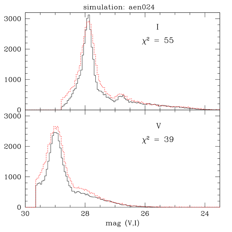
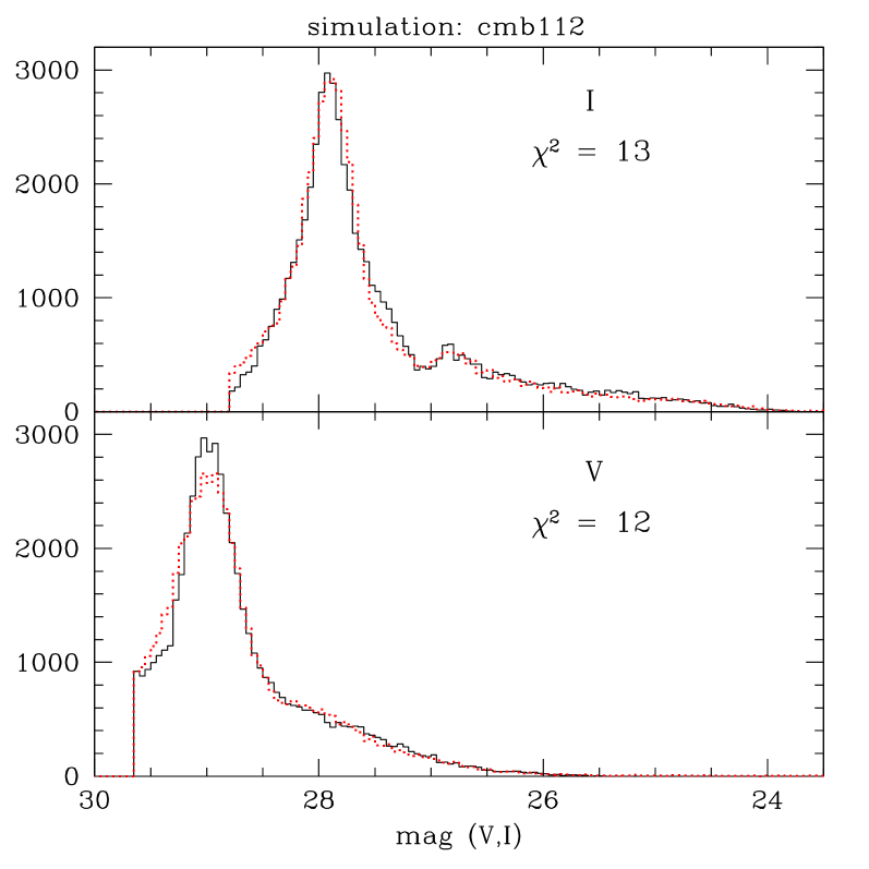
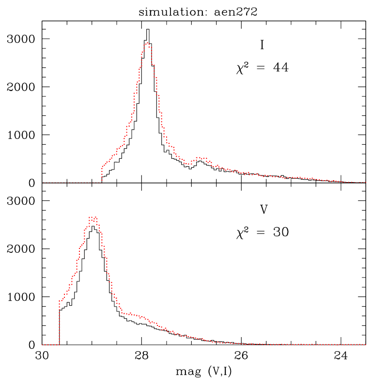
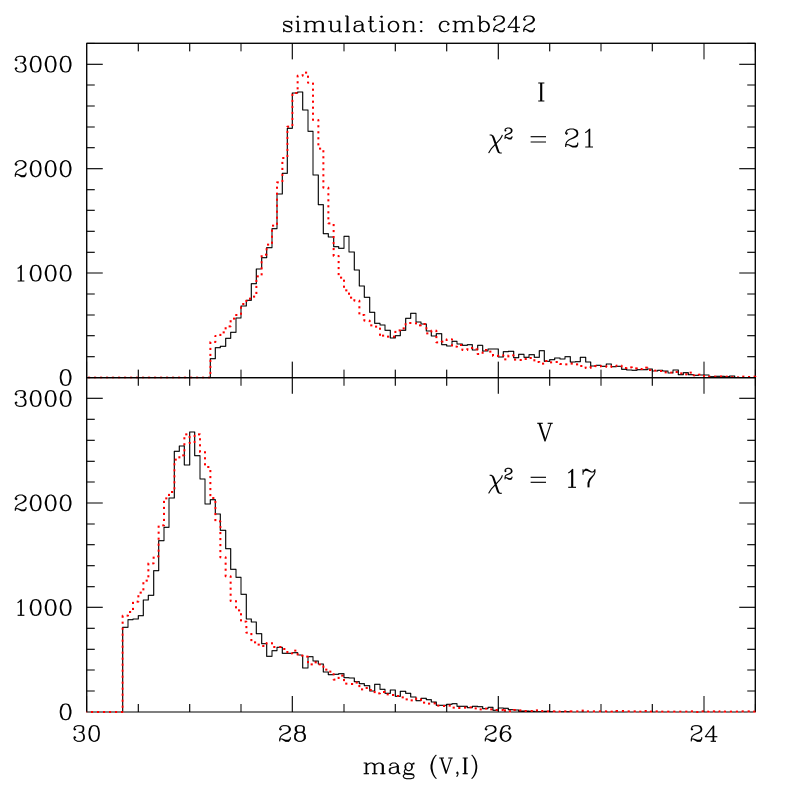
Figure 11: Comparison of the LF fits between the observations (dotted red line) and the simulations (solid black line), where only data above 50% completeness limits are considered. The left panels plot the best fitting LFs for the single age simulation that has 11 Gyr, and the right panels plot the LFs for the best fitting 2-burst simulation that has 80% 12 Gyr population and 20% 2.5 Gyr old population. The top panels are for the comparison with simulations that have input observed MDF, and the bottom panels show simulated LFs with input closed box enrichment. The single age closed box model is shown on the left and the two-burst model composed of input closed box simulations is on the right.

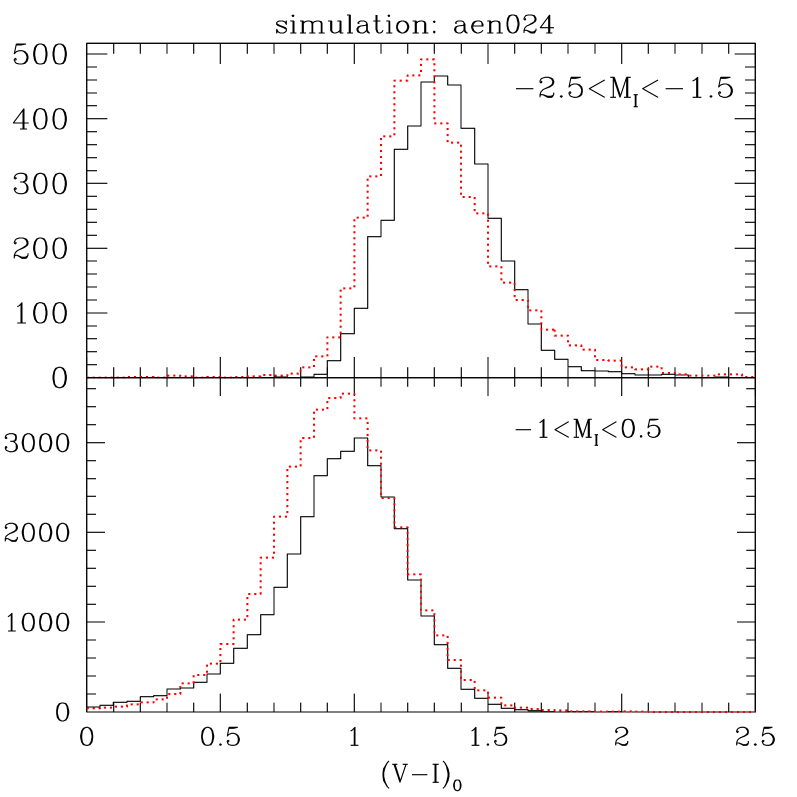
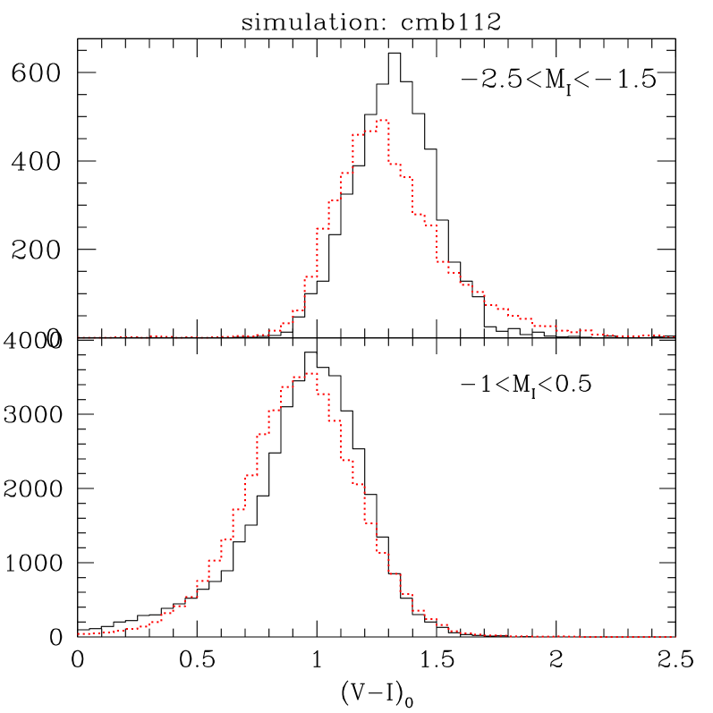
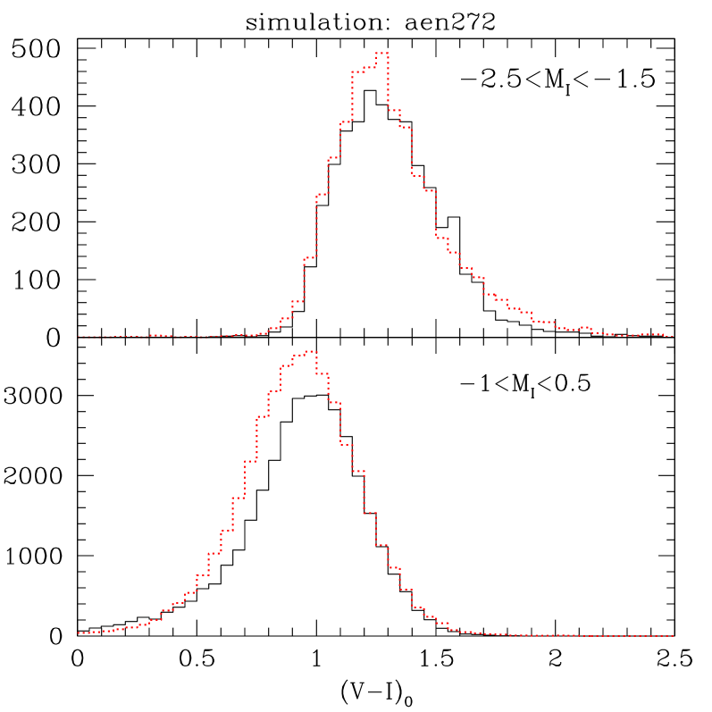
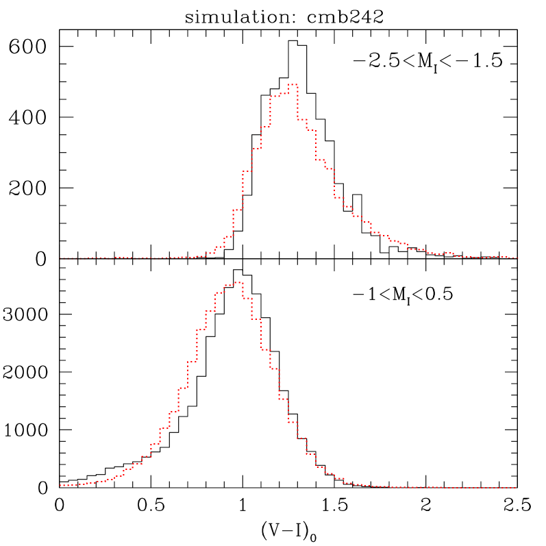
Figure 12: Comparison of V-I colour distributions between the data (dotted red line) and the simulations (solid black line), where only data in the specific luminosity range are considered. Upper panels show the colour distributions for the red giant branch stars that are selected in the magnitude range $-2.5<M_{I}<-1.5$ (where the bolometric corrections for the upper cool part of the RGB are not a problem), while the lower panels show the colour distributions for the part of the luminosity range dominated by helium burning stars (red clump) selected to be within range $-1<M_{I}<+0.5$ mag. Upper left diagrams are for the best fitting single age simulation (11 Gyr old model) with input observed MDF. Upper right diagrams are for the best fitting two burst model which is made by combining single age simulations with input observed MDFs (80% 12 + 20% 3 Gyr). The bottom panels show the best fitting simulations with input closed box metallicity distributions - the single age closed box model on the left and the two-burst model composed of input closed box simulations is on the right.

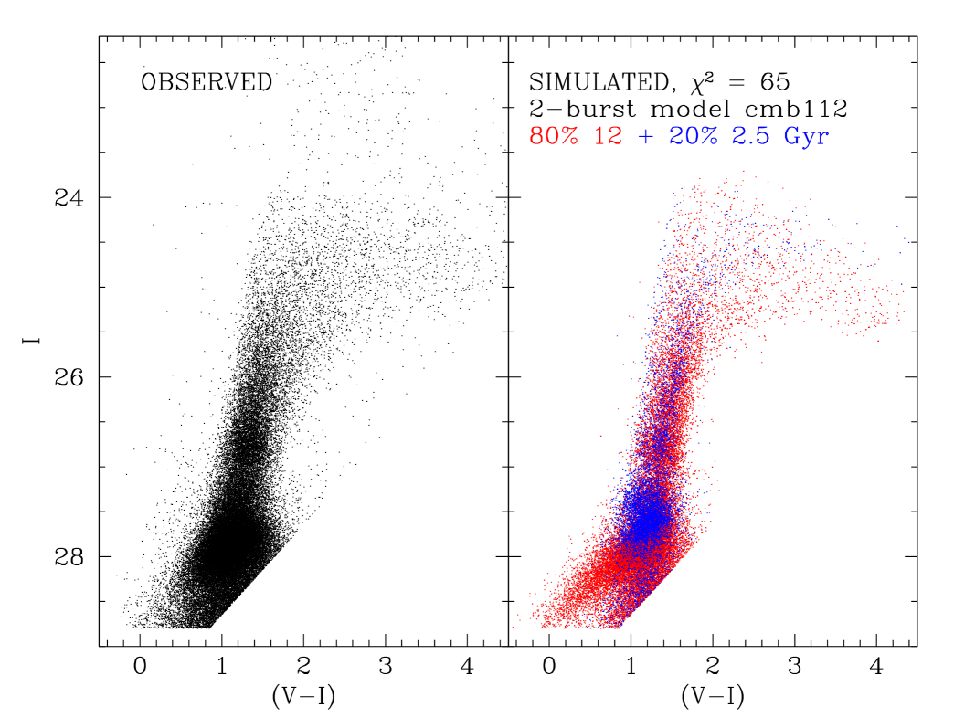
Figure 13: Comparison between the observed CMD (left) and the best fitting 2-burst simulation (right). The simulated stars are colour coded according to their age: 12 Gyr old stars are red, and 3 Gyr old stars are blue.

The $\chi^{2}$ values for the whole CMD fit for the best fitting 2-burst models are similar to those of the best fitting single age models: $\chi^{2}=65$ for 80% 12 Gyr + 20% 2.5 Gyr model and $\chi^{2}=66$ for the 11 Gyr single age simulation. The fact that there is almost no improvement in the full CMD fit between the single age and two-burst best fitting models, again confirms that the bulk of the stellar population in the observed CMD is old.

In contrast, the luminosity function fits are significantly improved over the single-age simulations (Figure 11). The $\chi^{2}$ values for the single age 12 Gyr old alpha enhanced simulation were 36 and 26 for the I and V-band luminosity functions. By contrast, for the 2-burst simulation with 70% 12.5 Gyr + 30% 6 Gyr the LF fits give $\chi^{2}=8$ and 12 for the I and V-band respectively. For the 12+2.5 Gyr model that has an 80% old population (that best fits the whole CMD), the LFs give $\chi^{2}=13$ and $12$ for I and V-band, respectively. However, the V-band LF has too many stars with respect to the data at the magnitude corresponding to the RC maximum (Figure 11).

The improvement with respect to single age simulations is visible also in the colour distribution of red clump and RGB regions (Figure 12), as well as in the number of AGB bump and RC stars in their respective boxes in the CMD (Table 4). Therefore the two burst star formation history is clearly favored over a single star formation event.

To understand the basic effect of adding a second component, we may ask just where in the CMD the younger component is contributing differently from the “baseline” old component. Figure 13 shows the best fitting 2-burst simulated CMD compared to the observations. The simulated CMD is colour coded according to the ages of simulated stars: here, we see that the “young” component (blue) contributes most strongly to the brighter, redder end of the red clump population. Without those stars, the luminosity function of the red clump is too narrow in magnitude to match the data and the model solution is not as successful.

4.3 Simulations with closed box chemical evolution

Table 5: The best fitting models for each diagnostic are listed for the single age and two burst simulations with input closed box MDF. Diagnostics are $\chi^{2}$ for the full CMD, $\chi^{2}$ of the LF fit for I, and V-bands, and in the last two columns $\Delta N/\sqrt{N_{obs}}=\mathrm{N}_{obs}-\mathrm{N}_{sim}/\sqrt{N_{obs}}$ for the RC and AGBb boxes in our grid.

Single age models with closed box MDF
simulation	age	$Z_{min}$	$Z_{max}$	yield	$\chi^{2}$	$\chi^{2}$	$\chi^{2}$	$\frac{\Delta N}{\sqrt{N_{obs}}}$	$\frac{\Delta N}{\sqrt{N_{obs}}}$
ID	Gyr				CMD	LFI	LFV	RC	AGBb
CMD:
aen272	10.5	0.0001	0.0400	0.0130	51.5	44.0	29.7	-0.7	12.5
aen273	11.0	0.0001	0.0400	0.0140	54.7	35.3	21.3	2.8	9.5
aen279	10.0	0.0001	0.0400	0.0130	54.8	66.4	38.5	0.2	11.9
LFI:
aen276	11.0	0.0001	0.0400	0.0170	62.4	27.4	12.0	-5.3	9.6
aen277	11.0	0.0001	0.0400	0.0180	69.2	33.0	15.3	-3.4	10.6
aen274	11.0	0.0001	0.0400	0.0150	60.7	34.5	21.3	2.5	11.2
LFV:
aen276	11.0	0.0001	0.0400	0.0170	62.4	27.4	12.0	-5.3	9.6
aen277	11.0	0.0001	0.0400	0.0180	69.2	33.0	15.3	-3.4	10.6
aen278	11.0	0.0001	0.0400	0.0190	74.6	34.7	16.8	-1.8	11.3
RC:
aen279	10.0	0.0001	0.0400	0.0130	54.8	66.4	38.5	0.2	11.9
aen254	8.0	0.0020	0.0200	0.0130	129.0	168.7	102.9	0.6	5.6
aen272	10.5	0.0001	0.0400	0.0130	51.5	44.0	29.7	-0.7	12.5
AGBb:
aen320	2.5	0.0080	0.0400	0.0130	498.5	501.8	239.0	48.4	-0.1
aen303	3.0	0.0050	0.0300	0.0130	444.9	496.4	256.0	52.0	-0.8
aen306	4.0	0.0050	0.0200	0.0130	383.7	430.2	252.0	41.9	0.5

Two burst models with closed box MDF
combined	old	young	age1	age2	%	%	$\chi^{2}$	$\chi^{2}$	$\chi^{2}$	$\frac{\Delta N}{\sqrt{N_{obs}}}$	$\frac{\Delta N}{\sqrt{N_{obs}}}$	$Z_{min},Z_{max},y$	$Z_{min},Z_{max},y$
simulation	P1	P2	Gyr	Gyr	P1	P2	CMD	LFI	LFV	RC	AGBb	P1	P2
CMD:
cmb242	aen270	aen316	12.0	2	80	20	56.7	21.3	17.4	8.8	-1.6	0.0001, 0.04, 0.013	0.002, 0.02, 0.013
cmb792	aen270	aen259	12.0	3	80	20	57.9	14.5	11.0	4.0	-2.1	0.0001, 0.04, 0.013	0.002, 0.02, 0.013
cmb257	aen270	aen321	12.0	2.5	80	20	60.5	18.4	16.4	5.8	-3.9	0.0001, 0.04, 0.013	0.005, 0.02, 0.013
cmb222	aen270	aen307	12.0	2	80	20	61.5	15.3	10.6	4.1	-0.5	0.0001, 0.04, 0.013	0.0001, 0.04, 0.013
LFI:
cmb971	aen270	aen304	12.0	4	80	20	85.2	8.9	11.5	-7.0	0.1	0.0001, 0.04, 0.013	0.005, 0.03, 0.013
cmb822	aen282	aen292	12.0	5	80	20	81.9	9.2	13.0	-5.9	0.4	0.0001, 0.04, 0.013	0.0001, 0.04, 0.013
cmb787	aen270	aen268	12.0	4	80	20	87.9	9.3	13.4	-7.5	-0.2	0.0001, 0.04, 0.013	0.005, 0.04, 0.02
cmb943	aen270	aen298	12.0	4	80	20	82.9	9.3	9.9	-4.8	0.2	0.0001, 0.04, 0.013	0.002, 0.04, 0.013
LFV:
cmb221	aen270	aen307	12.0	2	90	10	73.5	13.5	9.2	-3.8	2.1	0.0001, 0.04, 0.013	0.0001, 0.04, 0.013
cmb241	aen270	aen316	12.0	2	90	10	64.5	15.4	9.3	-2.0	1.3	0.0001, 0.04, 0.013	0.002, 0.02, 0.013
cmb236	aen270	aen315	12.0	2	90	10	64.0	15.8	9.6	-1.9	-1.3	0.0001, 0.04, 0.013	0.005, 0.02, 0.013
cmb943	aen270	aen298	12.0	4	80	20	82.9	9.3	9.9	-4.8	0.2	0.0001, 0.04, 0.013	0.002, 0.04, 0.013
RC:
cmb986	aen270	aen293	12.0	3	80	20	73.5	11.6	10.0	-0.3	1.1	0.0001, 0.04, 0.013	0.0001, 0.04, 0.013
cmb768	aen205	aen259	10.0	3	70	30	197.0	62.4	117.5	0.0	-8.1	0.0001, 0.01, 0.008	0.002, 0.02, 0.013
cmb766	aen205	aen259	10.0	3	90	10	245.4	36.1	131.7	0.2	-2.6	0.0001, 0.01, 0.008	0.002, 0.02, 0.013
cmb744	aen279	aen259	10.0	3	60	40	160.6	87.6	49.8	0.4	-4.0	0.0001, 0.04, 0.013	0.002, 0.02, 0.013
AGBb:
cmb940	aen270	aen297	12.0	3	80	20	81.7	10.7	10.6	-1.1	0.0	0.0001, 0.04, 0.013	0.002, 0.04, 0.015
cmb838	aen272	aen292	10.5	5	70	30	90.2	44.3	17.0	-22.9	0.0	0.0001, 0.04, 0.013	0.0001, 0.04, 0.013
cmb713	aen273	aen267	11.0	5	70	30	93.8	29.2	15.1	-21.3	0.0	0.0001, 0.04, 0.014	0.005, 0.04, 0.02
cmb785	aen270	aen266	12.0	6	50	50	128.1	22.0	14.4	-11.9	0.0	0.0001, 0.04, 0.013	0.005, 0.04, 0.02

To explore single age and two-burst models with an alternative, physically motivated input MDF we compare the observations with models that follow the classic closed box chemical enrichment. While strictly speaking, a closed-box model cannot be an instantaneous burst (as are the models in the previous sections), we assume here that the duration of the closed-box enrichment sequence is “fast” relative to the time resolution of the model grid, which is near 1 Gyr. This is consistent with the adoption of alpha enhanced stellar evolution models.

We explored a wide range of closed-box yields, minimum and maximum metallicities, and found the best fit to the observed CMD is provided by models with ages 10.5-11 Gyr, yield $y\sim 0.65-0.7Z_{\odot}$, and metallicity spanning the full range of the adopted set of models, with the minimum $Z_{min}=0.0001$ and maximum metallicity $Z_{max}=+0.04$. The $\chi^{2}$ values of the best fitting single age model with the input closed box enrichment (model aen272, age 10.5 Gyr,) are: $\chi^{2}(\mathrm{CMD})=52$, $\chi^{2}(\mathrm{LF}_{I})=44$, and $\chi^{2}(\mathrm{LF}_{V})=30$. The 11 Gyr old population model with slightly higher effective yield provide even smaller $\chi^{2}$ values of 27 and 12 for the I and V-band LFs, respectively (see Table 8 for details). As found in the case of single burst models with input observed MDF, the LF fits favor slightly older age than the full CMD fit. However, overall the result is essentially the same with the best fitting single age model of 10.5-11 Gyr.

We note that for the full CMD fit, LF fit (Fig. 11) and colour distribution comparison with data (Fig. 12) the closed box single age models are a slightly better match than the single age simulations with the input observed MDF. Also, as found for the models with the input observed MDF, the simulations with alpha enhanced isochrones provide better fit to the observations.

As done for models with the input MDF we combine the single age closed box models in order to explore the two-burst scenario. However, now in addition to the parameter of age, we have three more parameters: the effective yield, minimum and maximum metallicity. Therefore the number of possible two burst combinations is significantly increased.

The full set of models that have been constructed by combining two closed box single age simulations, by randomly extracting a fraction P1 of old stars and a fraction P2 of younger stars, in the same way as described above for two burst simulations with input observed MDF, is provided in the electronic format in Table 10.

Summarizing the results, we confirm the finding from the two-burst input MDF simulations above: the best fitting models have $\sim 80$% of 12 Gyr old population mixed with $\sim 20$% 2-4 Gyr old stars. The $\chi^{2}$ of the full CMD fit for the two burst model does not improve over the single age models with input closed box enrichment, but the luminosity functions fit the data much better. Also the numbers of RC and AGB bump stars in the respective boxes on the CMD are in better agreement with the observations for two burst models. In particular this is a significant difference for the number of AGB bump stars that in single age models is systematically lower than in the observations.

Exploring the different minimum and maximum metallicity for the old and for the young component we gain in addition some insight in the possible age-metallicity relation. The best fitting two-burst closed box model is cmb242 that is a combination of 80% 12 Gyr old model aen270 that has effective yield 0.013, and that spans the full scale of metallicity, from $Z_{min}=0.0001$ to $Z_{max}=0.04$. The young component contributing 20% of the stars is best represented by model aen316, which has the same effective yield, but a higher minimum metallicity $Z_{min}=0.002$. The maximum metallicity extends to the solar value $Z_{max}=0.02$. The simulations that had the young component with wider metallicity distribution, and in particular with a metal-poor component had worse CMD fits. Similarly, the simulations constructed with the old component that does not span the full metallicity range provide worse fits. Therefore we can conclude that it is not only necessary to have the bulk of population with age older than $\sim 10$ Gyr, but also that the old stars must cover the full range of metallicity.

5 Discussion

Figure 14: Age distribution (top panel) and metallicity distribution (bottom panel) for an example of complex star formation history that has stars formed first between 10.5-12.5 Gyr, and then a second very short burst at 3 Gyr. The top panel shows the percentage of the stars in each age bin as a function of age, while in the bottom panel the percentage of stars is given for each metallicity bin, normalized to the total number of stars in a given age. In the insert on the bottom panel the simulated total metallicity distribution is shown.

The best fitting mean age of the halo stars in NGC 5128 is $11\pm 1$ Gyr. This is older than the mean luminosity-weighted age of $\sim 8$ Gyr we derived in Paper I from the comparison of the observed luminosity function with the luminosity functions computed from BASTI models. In part the difference may be explained by the fact that in Paper I we did not take into account the effects of photometric scatter in the models, and in part by the fact that we used a different model grid for the MDF derivation (the alpha-enhanced Victoria isochrones from VandenBerg et al. (2000)) with respect to the LF modeling (BASTI Pietrinferni et al. 2004). In the present paper we self-consistently used the same stellar evolutionary models to derive the empirical MDF and in the simulations. One additional (though small) difference is the fact that in our new MDF, given in Table 1, we make a correction for the average AGB contribution.

The two-burst models with $\sim$70-80% of 12 Gyr old population combined with 30-20% 2-3 Gyr old second (younger) population give us the best match to the observed CMD. The 2-burst model LFs as well as number counts around RC and AGB bump features significantly improve the fit to the data over single-age models, and provide similar constraints to the full CMD fits: 70-80% of the population has 12-12.5 old stars, and the younger component of 30-20% has ages between 2-6 Gyr.

The simulations allow us to estimate the total mass transformed into stars in the target field which accounts for the observed number of stars. For a flattened Salpeter IMF ($\phi(M)\propto M^{-1.3}$ between 0.1 and 0.5 $M_{\odot}$ and $\phi(M)\propto M^{-2.35}$ between 0.5 and 120 $M_{\odot}$) the best fitting single burst simulations indicate that such mass amounts to $\simeq 4.5\times 10^{7}$ $M_{\odot}$. The best fitting double burst models yield a slightly smaller value of the total star formation in our field, i.e. $\simeq 4\times 10^{7}$ $M_{\odot}$, since young populations are more efficient in producing post main sequence stars per unit mass. The mass fraction involved in the young component is sensitive to its precise age, and amounts to $\sim 0.1$ if the young burst occurred 4 to 5 Gyr ago, or to $\sim 0.06$ if it occurred 2 to 3 Gyr ago.

We turn now to consider more complex star formation histories with the specific aim of testing some interesting scenarios.

5.1 Comparison of the stellar and globular cluster age and metallicity distributions

Woodley et al. (2010b) presented the most recent age and metallicity distributions of a large sample of globular clusters in NGC 5128 based on high quality Lick index measurements. The majority of their clusters are located in the inner halo and bulge ($R_{gc}\lesssim 15$ kpc), whereas our sample of stars is a “pencil beam” at one particular location in the halo. Nevertheless it is instructive to compare the age and metallicity distributions of two populations.

Fitting the age distribution histogram of their observed clusters with Gaussians they derive the best fitting mean age of the clusters for a single Gaussian fit of $8.58$ Gyr with $\sigma=2.78$ Gyr, younger than the mean age of the stars we find in this paper, but consistent with our results in Paper I. The best fitting bimodal distribution of clusters has 71% of the clusters with $\tau_{1}=10.12$ Gyr ($\sigma=1.44$) and 29% with age $\tau_{2}=4.85$ Gyr ($\sigma=1.32$). This is remarkably close to the proportions we find here for the halo stars in our two-burst models for the stellar CMD. The minor residual differences in the exact age values may well be due simply to the fact that the cluster ages and stellar ages were derived through different methodology and with reference to different stellar model grids. On the other hand the majority of the globular clusters observed by Woodley et al. (2010b) are more metal-poor than the bulk of the stellar halo.

Table 6: The three best fitting models for each diagnostic are listed for the three burst combinations with the input observed MDF. Diagnostics are $\chi^{2}$ for the full CMD, $\chi^{2}$ of the LF fit for I, and V-bands, and in the last two columns $\Delta N/\sqrt{N_{obs}}=\mathrm{N}_{obs}-\mathrm{N}_{sim}/\sqrt{N_{obs}}$ for the RC and AGBb boxes in our grid.

Three burst models with input observed MDF
combined	P1	P2	P3	age1	age2	age3	%	%	%	$\chi^{2}$	$\chi^{2}$	$\chi^{2}$	$\frac{\Delta N}{\sqrt{N_{obs}}}$	$\frac{\Delta N}{\sqrt{N_{obs}}}$
simulation	simulation	simulation	simulation	(Gyr)	(Gyr)	(Gyr)	(P1)	(P2)	(P3)	CMD	LFI	LFV	RC	AGBb
CMD:
new526	aen022	aen032	aen040	12.0	7.0	3.0	70	10	20	64.7	12.2	14.4	-5.3	-2.5
new538	aen022	aen034	aen040	12.0	6.0	3.0	70	10	20	67.2	14.0	13.4	-3.4	-1.9
cmb503	aen021	aen028	aen040	12.5	9.0	3.0	68	14	18	67.9	10.6	10.8	-1.2	-2.6
LFI:
cmb536	aen020	aen032	aen036	13.0	7.0	5.0	68	14	18	78.8	7.6	10.7	0.1	-2.7
cmb507	aen021	aen028	aen038	12.5	9.0	4.0	68	14	18	75.7	8.2	14.4	-6.2	-0.7
cmb524	aen020	aen030	aen036	13.0	8.0	5.0	68	14	18	83.8	8.2	10.2	1.3	-2.4
LFV:
cmb544	aen020	aen034	aen038	13.0	6.0	4.0	68	14	18	77.1	11.7	9.0	5.2	-4.0
new540	aen020	aen034	aen040	13.0	6.0	3.0	70	10	20	78.3	15.1	9.0	9.4	-5.7
cmb548	aen020	aen034	aen036	13.0	6.0	5.0	68	14	18	80.6	10.1	9.3	3.8	-3.8
RC:
new575	aen021	aen032	aen040	12.5	7.0	3.0	80	5	15	76.1	11.1	14.1	-0.1	-1.4
cmb536	aen020	aen032	aen036	13.0	7.0	5.0	68	14	18	78.8	7.6	10.7	0.1	-2.7
cmb512	aen020	aen028	aen036	13.0	9.0	5.0	68	14	18	82.2	8.8	11.2	-0.3	-2.4
AGBb:
new506	aen022	aen028	aen038	12.0	9.0	4.0	70	10	20	71.1	12.1	12.9	-10.5	0.0
new534	aen022	aen032	aen036	12.0	7.0	5.0	70	10	20	73.4	12.4	14.7	-12.4	0.1
cmb511	aen021	aen028	aen036	12.5	9.0	5.0	68	14	18	76.5	8.8	12.8	-6.7	-0.1

In addition to the single age and bimodal age distribution Woodley et al. (2010b) also fit their globular cluster age distribution with three Gaussians. They find that 68% of the NGC 5128 globular clusters are old ($\tau_{1}>8$ Gyr), 14% have intermediate age ($\tau_{2}=5-8$ Gyr), and 18% have young ages ($\tau_{3}<5$ Gyr). We explored the combination of old + intermediage-age + young single age models using both input MDF and closed box MDF. For these three-bursts star formation histories the fraction of the old component ($11-13$ Gyr) ranges between 60-80%, the fraction of the intermediate-age component ($6-9$ Gyr) between 5-15%, and the young component ($3-5$ Gyr) contributes 10-20% of the stars. None of the many combinations provided significantly better fits to the overall CMD and LFs with respect to the two burst simulations, but we note that the combination having similar percentages of the old, intermediate-age and young stars as was found for the clusters, is also consistent with the observed distribution of stars in the halo field CMD (see Table 6).

The stellar MDF measured in four fields in NGC 5128, from 8 to 40 kpc (Harris et al. 1999; Harris & Harris 2000, 2002; Rejkuba et al. 2005), does not show large differences. In all fields it is deficient in metal-poor stars, and has a peak at $\mathrm{[M/H]}\simeq-0.6$ dex. This metal-rich peak is very close to the metal-rich peak of the bimodal globular cluster metallicity distribution (Rejkuba 2001; Woodley et al. 2010b), while the metal-poor peak of the globular cluster MDF ($\mathrm{[Fe/H]}\sim-1.2$ dex) does not have the corresponding peak in the stellar MDF. This has already been noted in previous studies of NGC 5128 (Harris & Harris 2001, 2002), as well as in other galaxies (Harris & Harris 2001; Forte et al. 2007, e.g.). It implies that the efficiency of cluster formation relative to stars, measured by the globular cluster specific frequency $S_{N}$, is a function of metallicity and that metal-poor clusters have greater formation efficiency with respect to stars (Harris & Harris 2002). Forte et al. (2007) and Peng et al. (2008) discuss the possible implications of this proposed difference in efficiencies based on Monte Carlo based models and observations of many different galaxies.

One interesting implication predicted by Forte et al. (2007) is the coexistence of two distinct stellar populations characterized by widely different metallicities and spatial distributions. The metal-poor stellar halo is expected to be much more extended and start dominating over the metal-rich component only at large galactocentric distances. The inner, more metal-rich halo component is expected to be extremely heterogeneous and to dominate the inner region of galaxies (Forte et al. 2007). This is remarkably reminiscent of the emerging picture mentioned in the introduction, where stellar halos appear to have two components with the metal-poor population dominating at large distances in Milky Way, M31, NGC 3379 (Carollo et al. 2007; Chapman et al. 2006; Kalirai et al. 2006; Harris et al. 2007b). Moreover, small-scale sub-structures appear to be quite frequent in large galaxy halos (Bell et al. 2008; Ibata et al. 2009; Mouhcine et al. 2010b). However current data do not confirm whether this double nature of stellar halos is universal and the metal-poor component indeed dominating also in NGC 5128 at galactocentric distances larger than $\sim 12\mathrm{R}_{eff}$. For that new observations are necessary.

5.2 Duration of the star formation episodes

Besides exploring the age of the old/young components, it is also interesting to investigate whether it is possible to put constraints on the duration of the star formation burst(s). To test this we made a number of combinations of single age simulations with input observed MDF to test:

• Flat age distribution with constant star formation ranging over an extended period. Here we tested the constant star formation between 3-13, 5-13, and 9-13 Gyr.

• Flat age distribution for the old component with extended star formation between 9-13 Gyr, with a 20-40% contribution of young and intermediate-age stars with ages between 3-5 Gyr.

• Declining star formation lasting over more than 3 Gyr and starting $12$ Gyr ago.

• Bell shaped (first increasing, then decreasing), flat or declining star formation for the old population lasting 2-4 Gyr, with a very short younger burst contributing 20% of the stars.

This, admittedly limited in parameter space, set of more complex star formation histories shows much larger $\chi^{2}$ values ($>95$ for CMD fit) for all combinations when the old population was formed over an extended period longer than 3 Gyr, for both flat and declining age distributions. Better agreement with the observations is found for simulations where the old population has a mean age between 10-12.5 Gyr and a bell-shaped or flat distribution of ages, with the majority of the first generation of stars born within a short $\la 2$ Gyr period. In addition to the old population the younger component with star formation lasting only $\sim 1$ Gyr is necessary in order to bring the full CMD $\chi^{2}$ fit down to values similar to those obtained with the best fitting single and two burst simulations. An example of such a complex star formation history that has $\chi^{2}=63$ for the full CMD fit, and $\chi^{2}=18$ for the luminosity function fits is shown in Figure 14.

5.3 Age-metallicity relation

We explored the possibility of a variation of metallicity in lock steps with the age in the sense of increasing metallicity with decreasing age. The complex simulations were constructed by using in input several single age simulations with the flat metallicity distribution, from which we extracted stars, filling the metal-poor bins of the MDF with old stars and more metal-rich bins with increasingly younger stars. All of these cases gave significantly worse $\chi^{2}$ with respect to simulations that had old populations spanning the whole metallicity range. This is not too surprising, since the age-metallicity anti-correlation keeps the RGB narrow in colour. This confirms again the result found from 2-burst closed box simulations, that required the old component to span the full metallicity range from $Z=0.0001$ to $Z=0.04$.

6 Summary and conclusions

In this paper we have used a series of stellar population models to study the age distribution (ADF) and metallicity distribution (MDF) of the outer-halo stars in NGC 5128. Because it is only 3.8 Mpc distant, this target provides the best available opportunity to probe directly into the stellar population of a giant E galaxy. The reference data consist of our previously published deep HST/ACS photometry in $(V,I)$ which cover the RGB, HB (RC), and AGB stages (Rejkuba et al. 2005). We generate a large range of synthetic colour-magnitude diagrams from the Teramo stellar model grid (Pietrinferni et al. 2004, 2006; Cordier et al. 2007) and use a variety of diagnostics to constrain the best-fitting ADF and MDF. The simulations are compared with the observations and the following diagnostics are used to judge how well a simulation performs with respect to the others: $\chi^{2}$ of the full CMD fit based on a custom made grid, $\chi^{2}$ fits of the V and I-band luminosity functions, and relative number of RC and AGB bump stars based on star counts in the appropriate boxes on the CMD. The most sensitive diagnostics are the full CMD fit as well as the I-band LF.

Tables 3, 4, 5, and 6 list the values of our diagnostics for the three best fitting model CMDs for single age, two-burst, and three-burst simulations. Based on these and discussion above for additional more complex simulations the summary of our findings is as follows. The most convincing conclusions are:

1. Almost irrespective of the metallicity distribution adopted to simulate our field, the observational CMD requires an old age. This is mostly driven by the position of the RC. The best-fitting mean age for the halo stars is $11\pm 1$ Gyr.

2. Again, almost irrespective of the adopted metallicity distribution, the data are better fit with two episodes of star formation in which the old component dominates. This is mostly driven by the luminosity function of the RC stars. The best matches to the data are models with $\simeq 80$% of the stars at roughly 12 Gyr age, and only $\simeq 20$% in the range $2-4$ Gyr.

3. The old component must span the full metallicity range ($Z_{min}=0.0001$ to $Z_{max}=0.04$). This is driven by the width of the RGB.

In addition, we find formally better fits to both single age and two-burst models for input closed box MDF, with respect to the input observed MDF. This is driven by the colour distribution of the RC and the bright RGB. We however do not emphasize this point due to the uncertainties in the bolometric corrections and the additional parameter of element overabundance of the models. We also note that our best fitting multiple burst models have the young component which does not extend all the way to the low metallicity end ($Z\ga 0.002$), suggestive that the young component is, on the average, more metal rich than the old one.

The alpha enhanced isochrones provide superior fit to the data with respect to scaled solar ones. This is evident from the $\chi^{2}$ values of the overall CMD fit. Our tests of model to model comparisons (Sect. 3.3 and Fig. 4) clearly show that (i) when adequate input alpha enhanced tracks are used, the CMD $\chi^{2}$ diagnostic correctly reaches a value of 1 at the right age; (ii) when the input tracks have an inadequate $\alpha$ element distribution, the CMD $\chi^{2}$ diagnostic saturates at a relatively high value. Therefore, we suspect that more precise results could be obtained from simulations based on isochrones with a different chemical pattern, possibly with higher [$\alpha$/Fe] ratios. This however would hardly accommodate younger age for the old component, since, as [$\alpha$/Fe] increases, the isochrones become bluer.

We conclude that the age of the bulk of the stars in our NGC 5128 halo field are $\sim$ 11-12 Gyr old; a modest component with younger age ($\sim 2-4$ Gyr) is also present. If this region of NGC 5128 can be taken as representative of the halo, we would conclude that most of its stars and clusters formed at a very early time, in agreement with observational discoveries of old early-type galaxies at high redshift (Cimatti et al. 2004; Daddi et al. 2005; Renzini 2006; Kriek et al. 2008) as well as with lower redshift studies (e.g.  Silva & Bothun 1998; Kuntschner et al. 2002; Thomas et al. 2005). This is also in agreement with fast monolithic collapse models of Ikuta (2007), who considered the CMD morphology differences between fast early monolithic collapse and slow hierarchical merging early-type galaxy formation scenarios. Our solutions leave room for a significant merger or accretion event a few Gyr in the past, but they do not support the idea that the bulk of NGC 5128 stars formed in a “major merger” at $z<2$.

The “anomalous” features in NGC 5128, such as the central dust lane with its star forming regions and the ring of young massive stars (Graham 1979; Moellenhoff 1981; Quillen et al. 1993; Kainulainen et al. 2009) are significantly younger than the 2-4 Gyr younger halo component. Therefore it is possible that NGC 5128 has suffered several merger episodes. Possible evidence of an older accretion event in the halo is provided by the very diffuse star cluster candidate identified in our field (Mouhcine et al. 2010a). However, accurate deep photometry over the wide area of the halo would be necessary to find the stellar streams or subgroups of star clusters associated with the merger event that contributed the 20-30% younger component that is implied by the best fitting age distribution in our data. The turn off magnitude of the young component occurs at M${}_{I}\simeq 2$, M${}_{J,K}\simeq 1.5$. Therefore the presence of this young burst, its age and its stellar mass will be testable with JWST.

Appendix A Single age simulations diagnostics

This section lists the comparison between the single age simulations and observations for input observed MDF (Table 7) and for closed box model with a range of yields, and initial/final metallicities (Table 8). All the simulations that are made using solar scaled isochrones have names starting with ”sol*” and those that have alpha enhanced models are named ”aen*”. The $\chi^{2}$ goodness of the fit of the full CMD, the V- and I- band LFs as well as the comparison of the number of stars within the RC and AGBb boxes are used as diagnostics of the fit. Those diagnostics that indicate the best fit between the observations and models are indicated in bold faced letters. The bold text refers to the best three models listed in Table 3 and the first part of Table 5. This appendix and tables are only provided in the electronic edition.

Table 7: Diagnostics for all single age simulations with input observed MDF compared to observations. $\Delta N/\sqrt{N_{obs}}=\mathrm{N}_{obs}-\mathrm{N}_{sim}/\sqrt{N_{obs}}$ in columns 6, 7, 13, and 14 is the number difference between the observed and simulated stars in the parts of the CMD that are dominated by the RC (columns 6, 13) or AGBb stars (columns 7, 14), weighted by the Poissonian fluctuation in the number of stars expected from the observations. The first set (left) is for the models that included alpha enhancement (aen*), the second (right) for solar scaled models (sol*). The preferred models, those having smallest $\chi^{2}$ (or $\Delta N$ close to 0), for each diagnostic are indicated with bold-faced fonts. This table is given fully in the electronic version.

(1)	(2)	(3)	(4)	(5)	(6)	(7)	(8)	(9)	(10)	(11)	(12)	(13)	(14)
simulation	age	$\chi^{2}$	$\chi^{2}$	$\chi^{2}$	$\frac{\Delta N}{\sqrt{N_{obs}}}$	$\frac{\Delta N}{\sqrt{N_{obs}}}$	simulation	age	$\chi^{2}$	$\chi^{2}$	$\chi^{2}$	$\frac{\Delta N}{\sqrt{N_{obs}}}$	$\frac{\Delta N}{\sqrt{N_{obs}}}$
ID	(Gyr)	CMD	LFI	LFV	RC	AGBb	ID	(Gyr)	CMD	LFI	LFV	RC	AGBb
aen015	13.0	108.7	73.7	52.2	29.0	8.9	sol015	13.0	151.0	58.5	57.5	22.5	8.7
aen020	13.0	104.4	65.5	42.8	28.6	6.1	sol020	13.0	150.9	72.4	69.2	28.3	9.6
aen021	12.5	94.7	58.3	44.2	21.5	8.2	sol021	12.5	142.3	52.6	51.0	17.5	9.3
aen022	12.0	76.4	36.2	25.8	8.4	5.3	sol022	12.0	128.0	53.7	51.4	15.2	9.8
aen023	11.5	75.3	42.7	34.4	5.1	7.5	sol023	11.5	115.6	53.9	47.6	6.2	11.0
aen018	11.0	65.6	53.6	40.5	-0.9	8.8	sol018	11.0	107.2	48.4	36.7	-3.7	9.1
aen024	11.0	66.2	55.3	39.1	1.1	7.4	sol024	11.0	110.4	49.8	41.7	-1.4	10.5
aen025	10.5	65.2	55.7	34.5	-10.6	7.0	sol025	10.5	108.0	52.4	32.9	-10.9	8.0
aen016	10.0	67.1	72.4	41.0	-10.1	7.4	sol016	10.0	105.0	60.3	32.7	-13.4	11.0
aen017	10.0	67.7	74.1	39.3	-9.4	8.6	sol017	10.0	107.7	56.2	32.0	-15.0	9.2
aen026	10.0	68.9	69.9	38.4	-11.5	8.4	sol026	10.0	108.7	62.4	37.1	-7.7	8.4
aen027	9.5	76.0	82.7	39.0	-15.0	9.1	sol027	9.5	109.8	65.2	30.4	-17.2	8.2
aen028	9.0	81.4	114.4	50.9	-7.9	7.5	sol028	9.0	111.7	73.5	29.4	-16.9	8.9
aen029	8.5	90.3	131.3	54.9	-6.8	8.1	sol029	8.5	115.9	85.4	29.0	-16.2	8.0
aen030	8.0	95.7	140.4	56.5	-0.5	6.9	sol030	8.0	115.1	78.9	22.9	-15.8	7.4
aen031	7.5	107.1	158.6	68.0	6.5	8.4	sol031	7.5	115.4	96.7	26.6	-10.9	8.9
aen019	7.0	130.7	199.3	83.8	13.2	7.6	sol019	7.0	116.6	113.3	34.3	-3.3	8.7
aen032	7.0	128.6	210.7	94.6	17.0	10.0	sol032	7.0	116.1	110.9	32.4	-6.2	8.8
aen033	6.5	149.6	225.3	94.9	19.1	8.2	sol033	6.5	122.0	131.9	36.8	-0.1	7.8
aen034	6.0	173.0	241.4	103.5	24.2	6.8	sol034	6.0	133.1	146.5	41.3	3.2	8.7
aen035	5.5	210.8	292.7	125.1	29.4	7.3	sol035	5.5	140.5	166.8	47.7	9.6	7.3
aen036	5.0	237.3	331.6	157.7	39.1	8.0	sol036	5.0	153.4	207.5	68.6	19.0	6.6
aen037	4.5	285.6	370.8	180.1	45.2	7.7	sol037	4.5	177.6	254.1	90.7	26.3	9.7
aen038	4.0	320.0	419.4	226.8	51.9	7.1	sol038	4.0	199.7	282.2	105.4	30.6	7.1
aen039	3.5	375.1	513.2	282.4	58.7	7.3	sol039	3.5	231.7	349.8	147.8	38.6	6.7
aen040	3.0	423.9	608.7	364.8	66.8	8.1	sol040	3.0	274.4	426.2	210.5	48.1	6.1
aen041	2.5	511.2	684.6	428.0	73.6	7.5	sol041	2.5	347.8	526.8	275.0	59.7	7.5
aen042	2.0	643.7	801.0	568.3	80.9	10.2	sol042	2.0	427.7	640.7	379.7	68.7	6.7

Table 8: Diagnostics for all single age simulations with closed box input MDF compared to observations. Diagnostics are the same as in Table 7. The preferred models for each diagnostic are indicated with bold-faced fonts.

(1)	(2)	(3)	(4)	(5)	(6)	(7)	(8)	(9)	(10)
simulation	age	$Z_{min}$	$Z_{max}$	yield	$\chi^{2}$	$\chi^{2}$	$\chi^{2}$	$\frac{\Delta N}{\sqrt{N_{obs}}}$	$\frac{\Delta N}{\sqrt{N_{obs}}}$
ID	(Gyr)				CMD	LFI	LFV	RC	AGBb
sol200	12.0	0.0001	0.0100	0.0060	183.2	129.7	115.6	46.7	7.7
sol201	10.0	0.0001	0.0100	0.0060	134.6	86.5	147.2	20.3	10.1
sol202	8.0	0.0080	0.0400	0.0130	861.0	224.9	644.9	-49.5	12.9
sol203	5.0	0.0080	0.0400	0.0130	475.0	182.0	272.8	-27.2	10.7
sol204	12.0	0.0001	0.0100	0.0080	173.5	133.4	120.9	45.1	8.4
sol205	10.0	0.0001	0.0100	0.0080	121.3	86.3	134.4	17.2	9.1
sol206	8.0	0.0080	0.0400	0.0100	714.7	218.9	491.1	-47.0	11.7
sol207	5.0	0.0080	0.0400	0.0100	421.2	176.2	286.4	-24.5	8.1
sol208	3.0	0.0080	0.0400	0.0100	334.1	292.6	188.2	10.6	0.5
aen200	12.0	0.0001	0.0100	0.0060	325.5	183.5	174.7	62.9	12.2
aen201	10.0	0.0001	0.0100	0.0060	207.3	96.5	240.7	32.8	13.9
aen202	8.0	0.0080	0.0400	0.0130	459.2	197.6	282.5	-43.4	8.3
aen203	5.0	0.0080	0.0400	0.0130	387.9	212.2	168.5	-9.2	3.7
aen204	12.0	0.0001	0.0100	0.0080	290.9	173.6	171.1	60.5	10.8
aen205	10.0	0.0001	0.0100	0.0080	186.8	111.7	240.5	30.1	14.9
aen206	8.0	0.0080	0.0400	0.0100	380.4	181.0	298.0	-38.4	5.8
aen207	5.0	0.0080	0.0400	0.0100	347.2	218.4	139.7	-4.5	4.4
aen208	3.0	0.0080	0.0400	0.0100	436.9	440.2	218.9	41.1	0.9
aen230	12.0	0.0010	0.0100	0.0020	471.5	291.9	267.7	77.6	15.2
aen231	11.0	0.0010	0.0100	0.0020	400.8	132.4	285.6	61.7	15.1
aen232	10.0	0.0010	0.0100	0.0020	302.8	121.9	356.7	44.0	16.1
aen233	9.0	0.0010	0.0100	0.0020	300.0	217.0	385.8	29.2	14.7
aen234	8.0	0.0010	0.0100	0.0020	341.9	317.8	453.1	40.6	16.3
aen241	11.0	0.0010	0.0100	0.0100	162.9	77.0	153.0	27.7	7.1
aen242	10.0	0.0010	0.0100	0.0100	146.2	116.2	187.8	13.2	6.9
aen243	9.0	0.0010	0.0100	0.0100	168.7	198.0	229.7	11.7	8.5
aen244	8.0	0.0010	0.0100	0.0100	206.5	274.7	275.9	23.7	8.3
aen245	7.0	0.0010	0.0100	0.0100	272.5	367.3	337.4	39.4	10.4
aen246	6.0	0.0010	0.0100	0.0100	369.2	465.7	411.4	54.2	11.2
aen247	5.0	0.0010	0.0100	0.0100	471.2	601.9	531.0	68.0	11.7
aen251	11.0	0.0020	0.0200	0.0130	77.8	67.4	66.2	-6.0	4.5
aen252	10.0	0.0020	0.0200	0.0130	95.8	102.8	77.4	-11.8	4.5
aen253	9.0	0.0020	0.0200	0.0130	107.8	125.4	86.9	-9.3	5.5
aen254	8.0	0.0020	0.0200	0.0130	129.0	168.7	102.9	0.6	5.6
aen255	7.0	0.0020	0.0200	0.0130	171.8	230.4	132.5	13.0	5.7
aen256	6.0	0.0020	0.0200	0.0130	222.2	297.4	171.0	29.6	5.6
aen257	5.0	0.0020	0.0200	0.0130	282.4	360.5	217.7	41.6	5.1
aen258	4.0	0.0020	0.0200	0.0130	372.2	510.8	314.0	56.2	6.3
aen259	3.0	0.0020	0.0200	0.0130	473.4	707.6	487.1	74.5	7.1
aen261	11.0	0.0050	0.0400	0.0200	401.5	85.1	182.9	-51.4	7.8
aen262	10.0	0.0050	0.0400	0.0200	372.2	91.0	146.8	-47.5	7.3
aen263	9.0	0.0050	0.0400	0.0200	367.5	96.8	153.0	-45.7	8.7
aen264	8.0	0.0050	0.0400	0.0200	337.5	105.0	115.7	-33.6	9.6
aen265	7.0	0.0050	0.0400	0.0200	301.8	125.0	90.5	-22.5	8.4
aen266	6.0	0.0050	0.0400	0.0200	295.2	157.7	86.2	-12.4	5.9
aen267	5.0	0.0050	0.0400	0.0200	301.6	193.0	78.7	5.1	7.1
aen268	4.0	0.0050	0.0400	0.0200	316.2	302.6	106.3	23.6	6.6
aen269	3.0	0.0050	0.0400	0.0200	372.8	418.7	167.5	44.0	5.0
aen271	11.0	0.0001	0.0400	0.0130	66.3	42.2	34.4	11.2	11.9
aen281	10.0	0.0001	0.0400	0.0160	59.6	55.8	22.9	-7.5	13.4
aen291	8.0	0.0001	0.0400	0.0130	82.1	147.4	62.0	7.2	12.8
aen272	10.5	0.0001	0.0400	0.0130	51.5	44.0	29.7	-0.7	12.5

Table 8: cont.

(1)	(2)	(3)	(4)	(5)	(6)	(7)	(8)	(9)	(10)
simulation	age	$Z_{min}$	$Z_{max}$	yield	$\chi^{2}$	$\chi^{2}$	$\chi^{2}$	$\frac{\Delta N}{\sqrt{N_{obs}}}$	$\frac{\Delta N}{\sqrt{N_{obs}}}$
ID	(Gyr)				CMD	LFI	LFV	RC	AGBb
aen270	12.0	0.0001	0.0400	0.0130	94.7	50.2	33.1	23.2	11.6
aen273	11.0	0.0001	0.0400	0.0140	54.7	35.3	21.3	2.8	9.5
aen274	11.0	0.0001	0.0400	0.0150	60.7	34.5	21.3	2.5	11.2
aen275	11.0	0.0001	0.0400	0.0160	65.9	36.2	19.6	1.4	9.7
aen276	11.0	0.0001	0.0400	0.0170	62.4	27.4	12.0	-5.3	9.6
aen277	11.0	0.0001	0.0400	0.0180	69.2	33.0	15.3	-3.4	10.6
aen278	11.0	0.0001	0.0400	0.0190	74.6	34.7	16.8	-1.8	11.3
aen279	10.0	0.0001	0.0400	0.0130	54.8	66.4	38.5	0.2	11.9
aen280	10.0	0.0001	0.0400	0.0100	62.7	69.0	63.9	7.6	11.9
aen281	10.0	0.0001	0.0400	0.0160	59.6	55.8	22.9	-7.5	13.4
aen282	12.0	0.0001	0.0400	0.0130	92.3	48.4	30.9	23.6	10.1
aen283	12.0	0.0001	0.0400	0.0100	116.2	66.5	46.7	30.3	10.2
aen284	12.0	0.0001	0.0400	0.0160	90.2	42.5	26.1	18.2	10.5
aen285	12.0	0.0001	0.0100	0.0130	248.8	154.1	153.2	55.1	11.7
aen286	12.0	0.0001	0.0100	0.0100	267.4	166.7	173.7	57.0	13.1
aen287	12.0	0.0001	0.0100	0.0160	243.7	151.6	153.6	54.2	12.4
aen288	10.0	0.0001	0.0100	0.0130	159.4	98.4	196.2	23.9	11.0
aen289	10.0	0.0001	0.0100	0.0100	171.9	102.4	215.7	27.2	10.8
aen290	10.0	0.0001	0.0100	0.0160	158.1	104.2	206.1	23.9	11.2
aen291	8.0	0.0001	0.0400	0.0130	82.1	147.4	62.0	7.2	12.8
aen292	5.0	0.0001	0.0400	0.0130	227.2	326.5	153.9	43.7	10.5
aen293	3.0	0.0001	0.0400	0.0130	444.7	565.7	318.6	66.6	11.7
aen294	8.0	0.0020	0.0400	0.0130	116.9	132.7	45.5	-9.5	7.3
aen295	5.0	0.0020	0.0400	0.0130	233.3	274.1	105.1	29.7	7.5
aen296	3.0	0.0020	0.0400	0.0130	418.8	483.3	254.8	57.9	5.7
aen297	3.0	0.0020	0.0400	0.0150	366.2	494.5	239.2	57.9	7.5
aen298	4.0	0.0020	0.0400	0.0130	291.4	392.1	180.6	45.9	6.0
aen299	3.0	0.0020	0.0300	0.0130	416.4	587.6	348.0	66.5	7.0
aen300	4.0	0.0020	0.0300	0.0130	313.3	407.1	206.9	48.2	8.0
aen301	3.0	0.0050	0.0400	0.0130	376.0	467.4	226.1	51.9	5.5
aen302	4.0	0.0050	0.0400	0.0130	313.4	323.5	144.4	31.1	5.1
aen303	3.0	0.0050	0.0300	0.0130	444.9	496.4	256.0	52.0	-0.8
aen304	4.0	0.0050	0.0300	0.0130	354.1	336.1	157.0	32.0	2.5
aen305	3.0	0.0050	0.0200	0.0130	502.8	571.9	356.6	61.2	-2.1
aen306	4.0	0.0050	0.0200	0.0130	383.7	430.2	252.0	41.9	0.5
aen307	2.0	0.0001	0.0400	0.0130	702.8	780.9	514.8	81.2	12.1
aen308	2.5	0.0001	0.0400	0.0130	537.6	680.7	417.9	74.2	12.3
aen309	2.0	0.0001	0.0400	0.0170	567.9	801.0	472.2	79.1	11.1
aen310	2.0	0.0001	0.0400	0.0100	845.3	878.3	620.2	84.8	13.5
aen311	2.0	0.0010	0.0400	0.0130	645.2	737.4	464.0	78.5	7.8
aen312	2.0	0.0020	0.0400	0.0130	552.8	769.4	479.5	77.8	7.0
aen313	2.0	0.0050	0.0400	0.0130	481.3	702.2	396.6	71.8	4.1
aen314	2.0	0.0080	0.0400	0.0130	503.9	614.2	318.3	63.8	0.9
aen315	2.0	0.0050	0.0200	0.0130	660.7	819.9	605.8	80.7	1.0
aen316	2.0	0.0020	0.0200	0.0130	727.2	930.1	734.2	86.9	8.0
aen317	2.5	0.0010	0.0400	0.0130	449.8	705.2	423.3	74.1	12.9
aen318	2.5	0.0020	0.0400	0.0130	454.5	624.6	354.6	69.8	6.5
aen319	2.5	0.0050	0.0400	0.0130	453.3	544.8	272.1	58.7	2.9
aen320	2.5	0.0080	0.0400	0.0130	498.5	501.8	239.0	48.4	-0.1
aen321	2.5	0.0050	0.0200	0.0130	538.9	704.1	477.4	73.2	1.2
aen322	2.5	0.0020	0.0200	0.0130	599.3	776.6	554.0	79.4	3.9

Appendix B Double burst simulations diagnostics

This section lists the comparison between the combined simulations that simulate two burst star formation history. All the single age simulations that are made using solar scaled isochrones have names starting with ”sol*” and those that have alpha enhanced models are named ”aen*”. The combined simulations have names starting with ”cmb*”. The combinations are made by extracting randomly P1 % of stars from simulation 1 (old age) and P2 % of stars from simulation 2 (young age) and verifying that the observed MDF is populated correctly. The input simulations are single age simulations with either input observed MDF (Table 7) or with closed box model with a range of yields, and initial/final metallicities (Table 8). All the single age simulations used in input that are made using solar scaled isochrones have names starting with ”sol*” and those that have alpha enhanced models are named ”aen*”. The $\chi^{2}$ goodness of the fit of the full CMD, the V- and I- band LFs as well as the comparison of the number of stars within the RC and AGBb boxes are used as diagnostics of the fit. Those diagnostics that indicate the best fit between the observations and models are indicated in bold faced letters and correspond to the best three models reported in the second part of Table 5 and in Table 4. This appendix and tables are only provided in the electronic edition.

Table 9: Diagnostics for all 2-burst simulations composed by combining two single age simulations with input observed MDF compared to observations. The preferred models, those having smallest $\chi^{2}$ (or $\Delta N$ close to 0), for each diagnostic are indicated with bold-faced fonts. This table is given fully in the electronic version.

(1)	(2)	(3)	(4)	(5)	(6)	(7)	(8)	(9)	(10)	(11)	(12)
combined	old	young	age1	age2	%	%	$\chi^{2}$	$\chi^{2}$	$\chi^{2}$	$\frac{\mathrm{N}_{obs}-\mathrm{N}_{sim}}{\sqrt{N}}$	$\frac{\mathrm{N}_{obs}-\mathrm{N}_{sim}}{\sqrt{N}}$
simulation	simulation	simulation	(Gyr)	(Gyr)	(old)	(young)	CMD	LFI	LFV	RC	AGBb
cmb376	aen021	aen030	12.5	8	90	10	102.6	20.3	16.7	-5.8	1.4
cmb377	aen021	aen030	12.5	8	80	20	96.6	14.5	16.4	-9.2	1.2
cmb378	aen021	aen030	12.5	8	70	30	86.1	10.2	14.8	-11.1	2.0
cmb379	aen021	aen030	12.5	8	60	40	78.9	10.7	12.8	-13.5	1.6
cmb380	aen021	aen030	12.5	8	50	50	79.8	15.0	14.0	-15.6	1.7
cmb381	aen021	aen034	12.5	6	90	10	94.6	16.3	19.4	-4.6	-0.6
cmb382	aen021	aen034	12.5	6	80	20	83.8	10.9	15.3	-5.5	0.0
cmb383	aen021	aen034	12.5	6	70	30	74.3	8.3	12.3	-5.1	1.0
cmb384	aen021	aen034	12.5	6	60	40	71.7	10.7	12.9	-4.5	-1.1
cmb385	aen021	aen034	12.5	6	50	50	78.6	21.2	12.7	-6.5	-2.8
cmb386	aen021	aen038	12.5	4	90	10	93.4	15.6	15.6	-3.1	-2.0
cmb387	aen021	aen038	12.5	4	80	20	77.5	10.1	12.5	-0.0	-1.8
cmb388	aen021	aen038	12.5	4	70	30	73.9	12.6	12.1	1.6	-3.1
cmb389	aen021	aen038	12.5	4	60	40	84.8	21.3	17.5	5.1	-3.4
cmb390	aen021	aen038	12.5	4	50	50	113.6	39.5	20.6	9.7	-4.0
cmb391	aen021	aen040	12.5	3	90	10	81.6	15.3	15.8	-2.8	-1.2
cmb392	aen021	aen040	12.5	3	80	20	70.6	11.7	12.7	2.5	-3.3
cmb393	aen021	aen040	12.5	3	70	30	70.0	17.9	13.2	7.0	-4.8
cmb394	aen021	aen040	12.5	3	60	40	93.9	29.8	18.6	12.3	-2.8
cmb395	aen021	aen040	12.5	3	50	50	130.6	51.2	28.9	16.6	-3.9
cmb116	aen021	aen041	12.5	2.5	90	10	84.5	16.0	14.5	-0.8	-1.3
cmb117	aen021	aen041	12.5	2.5	80	20	71.3	15.3	12.8	6.6	-3.6
cmb118	aen021	aen041	12.5	2.5	70	30	72.5	22.7	15.5	11.8	-4.4
cmb119	aen021	aen041	12.5	2.5	60	40	105.8	40.3	24.4	17.2	-4.6
cmb120	aen021	aen041	12.5	2.5	50	50	158.7	62.0	38.2	22.6	-7.2
cmb141	aen021	aen042	12.5	2	90	10	80.2	16.6	11.9	0.1	-0.7
cmb142	aen021	aen042	12.5	2	80	20	65.6	16.2	11.2	7.1	-3.9
cmb143	aen021	aen042	12.5	2	70	30	77.9	26.4	16.7	15.1	-4.7
cmb144	aen021	aen042	12.5	2	60	40	123.4	48.6	28.2	23.7	-2.5
cmb145	aen021	aen042	12.5	2	50	50	195.1	76.3	48.7	29.8	-5.0
cmb476	aen021	sol030	12.5	8	90	10	111.6	22.8	18.7	-4.1	-1.3
cmb477	aen021	sol030	12.5	8	80	20	104.3	19.2	20.1	-8.0	3.2
cmb478	aen021	sol030	12.5	8	70	30	109.9	18.4	18.5	-9.4	2.1
cmb479	aen021	sol030	12.5	8	60	40	115.3	17.1	17.3	-12.9	1.2
cmb480	aen021	sol030	12.5	8	50	50	120.5	17.3	22.3	-16.1	3.4
cmb481	aen021	sol034	12.5	6	90	10	97.0	20.6	19.0	-4.2	1.6
cmb482	aen021	sol034	12.5	6	80	20	106.4	15.9	19.3	-6.1	1.3
cmb483	aen021	sol034	12.5	6	70	30	99.3	12.3	19.1	-8.9	2.2
cmb484	aen021	sol034	12.5	6	60	40	98.0	14.0	15.6	-10.7	1.6
cmb485	aen021	sol034	12.5	6	50	50	105.4	14.8	14.5	-12.6	2.2
cmb486	aen021	sol038	12.5	4	90	10	97.2	17.6	18.3	-6.4	0.4
cmb487	aen021	sol038	12.5	4	80	20	88.4	12.0	17.5	-5.5	-0.2
cmb488	aen021	sol038	12.5	4	70	30	85.8	11.8	15.5	-4.0	-2.5
cmb489	aen021	sol038	12.5	4	60	40	85.6	13.7	12.7	-2.7	0.0
cmb490	aen021	sol038	12.5	4	50	50	99.5	21.9	13.7	-4.1	-1.7
cmb491	aen021	sol040	12.5	3	90	10	91.3	18.0	20.5	-5.5	-0.8
cmb492	aen021	sol040	12.5	3	80	20	78.1	10.5	18.1	-4.2	-2.8
cmb493	aen021	sol040	12.5	3	70	30	81.0	11.2	16.6	-1.2	-2.7
cmb494	aen021	sol040	12.5	3	60	40	87.0	19.1	14.7	0.6	-4.8
cmb495	aen021	sol040	12.5	3	50	50	102.5	30.7	19.4	3.5	-5.9

Table 9: continue.

(1)	(2)	(3)	(4)	(5)	(6)	(7)	(8)	(9)	(10)	(11)	(12)
combined	old	young	age1	age2	%	%	$\chi^{2}$	$\chi^{2}$	$\chi^{2}$	$\frac{\mathrm{N}_{obs}-\mathrm{N}_{sim}}{\sqrt{N}}$	$\frac{\mathrm{N}_{obs}-\mathrm{N}_{sim}}{\sqrt{N}}$
simulation	simulation	simulation	(Gyr)	(Gyr)	(old)	(young)	CMD	LFI	LFV	RC	AGBb
cmb351	aen022	aen026	12.0	10	90	10	96.8	23.7	16.4	-13.9	-0.2
cmb352	aen022	aen026	12.0	10	80	20	96.1	22.1	15.3	-15.0	0.5
cmb353	aen022	aen026	12.0	10	70	30	93.2	21.6	15.8	-16.7	2.4
cmb354	aen022	aen026	12.0	10	60	40	86.8	19.9	16.8	-21.4	1.9
cmb355	aen022	aen026	12.0	10	50	50	81.3	20.7	14.7	-24.4	1.0
cmb356	aen022	aen030	12.0	8	90	10	91.1	19.4	17.3	-14.3	3.0
cmb357	aen022	aen030	12.0	8	80	20	87.8	17.8	16.9	-16.1	1.0
cmb358	aen022	aen030	12.0	8	70	30	86.3	13.6	15.0	-16.0	0.2
cmb359	aen022	aen030	12.0	8	60	40	83.4	15.5	13.9	-19.3	1.3
cmb360	aen022	aen030	12.0	8	50	50	83.0	18.9	13.7	-20.0	1.2
cmb361	aen022	aen034	12.0	6	90	10	87.9	16.7	17.4	-13.4	0.8
cmb362	aen022	aen034	12.0	6	80	20	85.3	13.0	14.9	-12.8	1.0
cmb363	aen022	aen034	12.0	6	70	30	76.8	12.7	16.7	-10.5	-2.0
cmb364	aen022	aen034	12.0	6	60	40	75.5	18.2	13.7	-11.6	-2.5
cmb365	aen022	aen034	12.0	6	50	50	80.8	25.8	14.0	-11.5	-2.2
cmb366	aen022	aen038	12.0	4	90	10	86.9	15.0	14.6	-12.0	0.2
cmb367	aen022	aen038	12.0	4	80	20	74.1	12.4	12.7	-7.4	-1.7
cmb368	aen022	aen038	12.0	4	70	30	70.7	13.6	12.2	-3.8	-3.4
cmb369	aen022	aen038	12.0	4	60	40	83.6	24.4	16.4	0.8	-1.6
cmb370	aen022	aen038	12.0	4	50	50	107.6	39.7	22.5	6.1	-4.8
cmb371	aen022	aen040	12.0	3	90	10	80.5	13.5	14.0	-8.4	-0.4
cmb372	aen022	aen040	12.0	3	80	20	67.0	12.4	12.3	-4.5	-1.2
cmb373	aen022	aen040	12.0	3	70	30	68.5	18.6	15.6	1.1	-3.2
cmb374	aen022	aen040	12.0	3	60	40	92.0	33.3	22.7	7.8	-5.4
cmb375	aen022	aen040	12.0	3	50	50	134.3	53.8	33.0	12.5	-4.7
cmb111	aen022	aen041	12.0	2.5	90	10	78.1	14.8	14.0	-8.3	-0.1
cmb112	aen022	aen041	12.0	2.5	80	20	65.0	13.4	12.3	-3.8	-1.6
cmb113	aen022	aen041	12.0	2.5	70	30	71.3	21.9	15.8	4.3	-5.4
cmb114	aen022	aen041	12.0	2.5	60	40	103.2	37.7	25.9	12.8	-7.2
cmb115	aen022	aen041	12.0	2.5	50	50	152.3	60.7	38.4	19.3	-6.3
cmb136	aen022	aen042	12.0	2	90	10	69.0	12.6	12.8	-7.6	0.0
cmb137	aen022	aen042	12.0	2	80	20	65.4	15.2	12.6	1.7	-3.1
cmb138	aen022	aen042	12.0	2	70	30	78.8	27.4	17.4	9.2	-4.3
cmb139	aen022	aen042	12.0	2	60	40	118.2	46.5	32.1	18.0	-3.0
cmb140	aen022	aen042	12.0	2	50	50	196.4	76.9	51.5	26.1	-4.8
cmb451	aen022	sol026	12.0	10	90	10	103.5	26.0	15.9	-11.5	2.8
cmb452	aen022	sol026	12.0	10	80	20	105.6	27.4	17.0	-10.3	3.6
cmb453	aen022	sol026	12.0	10	70	30	113.1	23.5	17.1	-9.0	4.4
cmb454	aen022	sol026	12.0	10	60	40	121.5	26.4	18.6	-12.6	4.7
cmb455	aen022	sol026	12.0	10	50	50	128.6	28.2	19.9	-12.9	3.0
cmb456	aen022	sol030	12.0	8	90	10	101.7	24.4	18.5	-13.7	-0.3
cmb457	aen022	sol030	12.0	8	80	20	104.0	20.4	17.0	-14.4	3.7
cmb458	aen022	sol030	12.0	8	70	30	109.6	19.8	17.1	-14.6	4.6
cmb459	aen022	sol030	12.0	8	60	40	109.6	18.8	17.0	-16.3	3.2
cmb460	aen022	sol030	12.0	8	50	50	116.3	21.6	19.2	-19.7	2.6
cmb461	aen022	sol034	12.0	6	90	10	98.2	20.7	17.9	-12.0	0.6
cmb462	aen022	sol034	12.0	6	80	20	90.8	15.9	17.0	-15.2	2.4
cmb463	aen022	sol034	12.0	6	70	30	95.8	16.5	15.0	-13.4	3.0
cmb464	aen022	sol034	12.0	6	60	40	97.7	17.8	13.9	-15.9	3.1
cmb465	aen022	sol034	12.0	6	50	50	107.6	21.1	15.6	-16.9	1.1
cmb466	aen022	sol038	12.0	4	90	10	88.4	17.5	16.7	-13.2	-0.4
cmb467	aen022	sol038	12.0	4	80	20	80.8	14.0	17.5	-12.3	1.6
cmb468	aen022	sol038	12.0	4	70	30	79.3	13.2	16.0	-12.6	-0.6
cmb469	aen022	sol038	12.0	4	60	40	82.7	16.4	13.3	-9.6	-0.2
cmb470	aen022	sol038	12.0	4	50	50	93.1	26.7	13.2	-9.5	-1.5

Table 9: continue.

(1)	(2)	(3)	(4)	(5)	(6)	(7)	(8)	(9)	(10)	(11)	(12)
combined	old	young	age1	age2	%	%	$\chi^{2}$	$\chi^{2}$	$\chi^{2}$	$\frac{\mathrm{N}_{obs}-\mathrm{N}_{sim}}{\sqrt{N}}$	$\frac{\mathrm{N}_{obs}-\mathrm{N}_{sim}}{\sqrt{N}}$
simulation	simulation	simulation	(Gyr)	(Gyr)	(old)	(young)	CMD	LFI	LFV	RC	AGBb
cmb471	aen022	sol040	12.0	3	90	10	83.6	17.1	15.4	-12.7	-0.3
cmb472	aen022	sol040	12.0	3	80	20	80.7	10.5	14.1	-9.4	0.2
cmb473	aen022	sol040	12.0	3	70	30	71.8	15.5	15.0	-5.9	-3.9
cmb474	aen022	sol040	12.0	3	60	40	83.9	22.4	16.0	-5.8	-3.1
cmb475	aen022	sol040	12.0	3	50	50	103.8	37.1	18.7	-1.6	-5.3
cmb326	aen018	aen028	11.0	9	90	10	93.6	32.0	16.2	-29.1	1.6
cmb327	aen018	aen028	11.0	9	80	20	92.8	35.7	16.6	-29.5	-0.2
cmb328	aen018	aen028	11.0	9	70	30	96.7	36.3	17.4	-33.1	2.3
cmb329	aen018	aen028	11.0	9	60	40	96.4	34.7	15.3	-32.1	2.2
cmb330	aen018	aen028	11.0	9	50	50	96.7	43.3	15.9	-33.6	1.2
cmb216	aen024	aen030	11.0	8	90	10	97.8	32.9	16.0	-30.8	2.0
cmb331	aen018	aen030	11.0	8	90	10	97.0	36.0	17.3	-31.5	3.0
cmb217	aen024	aen030	11.0	8	80	20	94.9	33.0	15.6	-29.8	2.9
cmb332	aen018	aen030	11.0	8	80	20	94.7	33.0	18.3	-30.2	1.0
cmb218	aen024	aen030	11.0	8	70	30	88.9	33.8	15.2	-29.5	-1.0
cmb333	aen018	aen030	11.0	8	70	30	90.4	31.8	15.8	-29.6	1.0
cmb219	aen024	aen030	11.0	8	60	40	91.7	37.1	16.2	-28.8	1.2
cmb334	aen018	aen030	11.0	8	60	40	92.5	36.8	16.3	-28.4	1.6
cmb220	aen024	aen030	11.0	8	50	50	96.7	39.8	14.8	-29.4	0.3
cmb335	aen018	aen030	11.0	8	50	50	98.1	41.7	18.1	-30.1	2.9
cmb336	aen018	aen032	11.0	7	90	10	90.5	30.1	17.0	-28.8	2.2
cmb337	aen018	aen032	11.0	7	80	20	89.4	32.3	15.7	-27.6	1.8
cmb338	aen018	aen032	11.0	7	70	30	86.7	30.2	15.2	-25.9	1.3
cmb339	aen018	aen032	11.0	7	60	40	89.0	33.0	16.4	-24.2	-0.7
cmb340	aen018	aen032	11.0	7	50	50	95.2	42.1	17.0	-24.9	2.5
cmb211	aen024	aen036	11.0	5	90	10	87.9	30.6	15.6	-25.4	0.0
cmb341	aen018	aen036	11.0	5	90	10	86.3	30.1	16.9	-28.8	-0.6
cmb212	aen024	aen036	11.0	5	80	20	79.7	30.6	15.6	-24.0	-2.5
cmb342	aen018	aen036	11.0	5	80	20	83.5	29.4	16.8	-24.5	1.8
cmb213	aen024	aen036	11.0	5	70	30	80.0	35.1	17.3	-19.4	-1.2
cmb343	aen018	aen036	11.0	5	70	30	82.6	31.5	15.9	-20.7	-0.9
cmb214	aen024	aen036	11.0	5	60	40	85.8	38.4	17.3	-15.4	-1.8
cmb344	aen018	aen036	11.0	5	60	40	88.1	40.8	19.5	-17.5	-1.4
cmb215	aen024	aen036	11.0	5	50	50	100.3	52.1	21.3	-9.4	-2.6
cmb345	aen018	aen036	11.0	5	50	50	97.7	47.2	21.6	-12.4	-0.7
cmb346	aen018	aen040	11.0	3	90	10	79.7	26.9	15.1	-24.5	-0.7
cmb347	aen018	aen040	11.0	3	80	20	73.8	31.7	17.7	-17.8	-3.3
cmb348	aen018	aen040	11.0	3	70	30	81.7	39.2	23.1	-11.4	-1.6
cmb349	aen018	aen040	11.0	3	60	40	103.4	51.4	28.8	-3.3	-2.9
cmb350	aen018	aen040	11.0	3	50	50	144.5	70.6	40.6	3.7	-4.4
cmb106	aen024	aen041	11.0	2.5	90	10	79.8	28.6	15.1	-22.8	-3.1
cmb107	aen024	aen041	11.0	2.5	80	20	71.0	30.2	18.7	-15.1	-3.8
cmb108	aen024	aen041	11.0	2.5	70	30	77.5	36.6	22.1	-8.1	-4.9
cmb109	aen024	aen041	11.0	2.5	60	40	116.7	54.1	32.6	3.0	-6.1
cmb110	aen024	aen041	11.0	2.5	50	50	158.2	75.4	48.3	9.2	-5.8
cmb131	aen024	aen042	11.0	2	90	10	70.9	25.3	16.0	-21.8	-2.6
cmb132	aen024	aen042	11.0	2	80	20	67.8	32.6	17.6	-12.8	-1.9
cmb133	aen024	aen042	11.0	2	70	30	83.5	41.1	24.7	-3.1	-5.6
cmb134	aen024	aen042	11.0	2	60	40	123.4	60.4	38.3	7.6	-4.0
cmb135	aen024	aen042	11.0	2	50	50	204.1	90.0	60.4	17.3	-5.0
cmb426	aen018	sol028	11.0	9	90	10	96.6	34.0	15.2	-27.1	2.3
cmb427	aen018	sol028	11.0	9	80	20	104.8	33.5	14.5	-26.4	4.6
cmb428	aen018	sol028	11.0	9	70	30	112.0	36.0	15.5	-27.9	4.8
cmb429	aen018	sol028	11.0	9	60	40	119.4	36.9	14.8	-27.7	4.0
cmb430	aen018	sol028	11.0	9	50	50	128.8	34.3	17.2	-29.2	5.6

Table 9: continue.

(1)	(2)	(3)	(4)	(5)	(6)	(7)	(8)	(9)	(10)	(11)	(12)
combined	old	young	age1	age2	%	%	$\chi^{2}$	$\chi^{2}$	$\chi^{2}$	$\frac{\mathrm{N}_{obs}-\mathrm{N}_{sim}}{\sqrt{N}}$	$\frac{\mathrm{N}_{obs}-\mathrm{N}_{sim}}{\sqrt{N}}$
simulation	simulation	simulation	(Gyr)	(Gyr)	(old)	(young)	CMD	LFI	LFV	RC	AGBb
cmb431	aen018	sol030	11.0	8	90	10	98.5	33.9	14.8	-27.4	2.0
cmb432	aen018	sol030	11.0	8	80	20	98.5	33.4	16.7	-27.4	4.1
cmb433	aen018	sol030	11.0	8	70	30	106.2	33.2	15.0	-28.9	4.1
cmb434	aen018	sol030	11.0	8	60	40	117.7	37.9	15.8	-28.4	4.7
cmb435	aen018	sol030	11.0	8	50	50	127.1	36.9	15.1	-28.0	2.8
cmb436	aen018	sol032	11.0	7	90	10	97.1	32.7	14.2	-28.2	1.6
cmb437	aen018	sol032	11.0	7	80	20	95.7	32.4	14.3	-28.8	3.8
cmb438	aen018	sol032	11.0	7	70	30	101.4	34.9	16.8	-30.7	4.6
cmb439	aen018	sol032	11.0	7	60	40	108.3	36.4	14.4	-29.4	4.9
cmb440	aen018	sol032	11.0	7	50	50	121.4	40.2	14.2	-29.1	5.6
cmb441	aen018	sol036	11.0	5	90	10	91.8	36.5	15.2	-27.2	1.6
cmb442	aen018	sol036	11.0	5	80	20	94.0	30.7	16.8	-26.8	1.2
cmb443	aen018	sol036	11.0	5	70	30	97.0	35.3	15.7	-26.0	0.8
cmb444	aen018	sol036	11.0	5	60	40	99.9	37.1	14.0	-25.0	0.0
cmb445	aen018	sol036	11.0	5	50	50	109.8	42.0	14.1	-21.5	0.9
cmb446	aen018	sol040	11.0	3	90	10	89.1	29.3	18.0	-27.2	0.2
cmb447	aen018	sol040	11.0	3	80	20	85.5	27.8	17.9	-26.3	-1.6
cmb448	aen018	sol040	11.0	3	70	30	83.6	31.2	17.6	-19.1	-2.0
cmb449	aen018	sol040	11.0	3	60	40	96.1	41.0	20.5	-13.5	-3.4
cmb450	aen018	sol040	11.0	3	50	50	122.5	56.5	24.1	-10.7	-4.9
cmb201	sol024	sol036	11.0	5	90	10	191.0	40.3	40.9	-18.4	6.6
cmb202	sol024	sol036	11.0	5	80	20	179.8	34.8	37.3	-21.4	4.5
cmb203	sol024	sol036	11.0	5	70	30	165.9	35.2	27.8	-19.7	4.2
cmb204	sol024	sol036	11.0	5	60	40	154.8	32.2	22.2	-21.0	3.6
cmb205	sol024	sol036	11.0	5	50	50	156.6	38.0	16.4	-18.7	0.8
cmb206	sol024	sol030	11.0	8	90	10	208.2	44.5	44.5	-17.2	6.8
cmb207	sol024	sol030	11.0	8	80	20	200.3	41.6	43.7	-21.3	6.4
cmb208	sol024	sol030	11.0	8	70	30	202.1	43.4	41.8	-23.1	7.4
cmb209	sol024	sol030	11.0	8	60	40	187.3	41.4	35.8	-22.1	8.6
cmb210	sol024	sol030	11.0	8	50	50	181.5	36.5	36.0	-25.3	7.1
cmb301	aen026	aen030	10.0	8	90	10	106.3	51.9	16.2	-36.8	2.5
cmb302	aen026	aen030	10.0	8	80	20	112.7	52.8	16.8	-37.8	1.4
cmb303	aen026	aen030	10.0	8	70	30	110.9	56.0	16.8	-36.1	0.7
cmb304	aen026	aen030	10.0	8	60	40	112.4	61.5	19.4	-36.5	1.2
cmb305	aen026	aen030	10.0	8	50	50	116.4	61.3	17.9	-34.1	1.1
cmb306	aen026	aen034	10.0	6	90	10	111.5	52.6	19.3	-37.4	0.9
cmb307	aen026	aen034	10.0	6	80	20	107.3	59.9	20.6	-33.9	-1.1
cmb308	aen026	aen034	10.0	6	70	30	108.6	60.2	18.9	-32.1	-1.8
cmb309	aen026	aen034	10.0	6	60	40	117.4	65.1	19.4	-28.1	-1.5
cmb310	aen026	aen034	10.0	6	50	50	121.9	75.0	21.8	-24.8	-2.1
cmb311	aen026	aen036	10.0	5	90	10	107.1	54.6	18.6	-36.7	1.3
cmb312	aen026	aen036	10.0	5	80	20	109.1	57.7	19.1	-33.0	0.2
cmb313	aen026	aen036	10.0	5	70	30	108.0	61.9	20.0	-27.2	-2.3
cmb314	aen026	aen036	10.0	5	60	40	114.4	66.6	20.7	-22.0	-1.9
cmb315	aen026	aen036	10.0	5	50	50	137.9	83.4	25.7	-17.9	-3.0
cmb316	aen026	aen038	10.0	4	90	10	107.2	51.7	18.8	-34.8	0.9
cmb317	aen026	aen038	10.0	4	80	20	109.0	54.8	19.0	-29.4	-0.5
cmb318	aen026	aen038	10.0	4	70	30	115.2	67.4	23.4	-23.5	-1.5
cmb319	aen026	aen038	10.0	4	60	40	127.9	75.4	26.1	-16.7	-2.3
cmb320	aen026	aen038	10.0	4	50	50	154.6	90.4	32.1	-8.3	-3.0
cmb321	aen026	aen040	10.0	3	90	10	100.2	52.6	17.8	-32.9	-0.1
cmb322	aen026	aen040	10.0	3	80	20	103.5	56.1	19.8	-27.5	-2.8
cmb323	aen026	aen040	10.0	3	70	30	114.9	69.6	27.5	-17.5	-1.5
cmb324	aen026	aen040	10.0	3	60	40	136.5	83.0	32.5	-9.2	-4.2
cmb325	aen026	aen040	10.0	3	50	50	180.9	107.1	47.2	-0.2	-3.6

Table 9: continue.

(1)	(2)	(3)	(4)	(5)	(6)	(7)	(8)	(9)	(10)	(11)	(12)
combined	old	young	age1	age2	%	%	$\chi^{2}$	$\chi^{2}$	$\chi^{2}$	$\frac{\mathrm{N}_{obs}-\mathrm{N}_{sim}}{\sqrt{N}}$	$\frac{\mathrm{N}_{obs}-\mathrm{N}_{sim}}{\sqrt{N}}$
simulation	simulation	simulation	(Gyr)	(Gyr)	(old)	(young)	CMD	LFI	LFV	RC	AGBb
cmb101	aen026	aen041	10.0	2.5	90	10	97.3	50.7	14.9	-32.0	-0.3
cmb102	aen026	aen041	10.0	2.5	80	20	103.2	60.2	21.5	-23.9	-3.3
cmb103	aen026	aen041	10.0	2.5	70	30	116.4	69.5	27.0	-14.1	-5.2
cmb104	aen026	aen041	10.0	2.5	60	40	147.4	87.0	37.7	-5.8	-3.0
cmb105	aen026	aen041	10.0	2.5	50	50	203.8	111.1	53.0	4.7	-6.7
cmb126	aen026	aen042	10.0	2	90	10	100.8	50.6	16.5	-30.4	-0.0
cmb127	aen026	aen042	10.0	2	80	20	102.0	59.2	22.3	-20.5	-2.0
cmb128	aen026	aen042	10.0	2	70	30	114.3	65.6	28.1	-9.9	-1.5
cmb129	aen026	aen042	10.0	2	60	40	165.3	89.7	41.1	0.4	-5.0
cmb130	aen026	aen042	10.0	2	50	50	244.3	115.0	65.8	12.0	-4.0
cmb401	aen026	sol030	10.0	8	90	10	108.3	47.4	15.6	-35.6	3.9
cmb402	aen026	sol030	10.0	8	80	20	118.3	52.1	11.9	-35.7	1.5
cmb403	aen026	sol030	10.0	8	70	30	127.1	46.6	13.8	-35.3	3.8
cmb404	aen026	sol030	10.0	8	60	40	132.8	51.2	15.2	-36.0	2.7
cmb405	aen026	sol030	10.0	8	50	50	141.9	50.0	14.3	-34.3	4.2
cmb406	aen026	sol034	10.0	6	90	10	112.7	51.9	18.1	-38.1	2.1
cmb407	aen026	sol034	10.0	6	80	20	114.0	53.9	14.9	-35.4	3.4
cmb408	aen026	sol034	10.0	6	70	30	122.4	54.8	14.4	-35.4	4.3
cmb409	aen026	sol034	10.0	6	60	40	127.4	58.3	15.2	-32.6	3.1
cmb410	aen026	sol034	10.0	6	50	50	134.4	67.4	16.2	-30.6	4.1
cmb411	aen026	sol036	10.0	5	90	10	109.3	49.4	15.5	-36.5	1.2
cmb412	aen026	sol036	10.0	5	80	20	111.3	56.8	16.5	-33.9	0.5
cmb413	aen026	sol036	10.0	5	70	30	117.4	56.5	17.1	-34.4	0.1
cmb414	aen026	sol036	10.0	5	60	40	123.0	61.2	16.2	-30.1	1.0
cmb415	aen026	sol036	10.0	5	50	50	136.1	71.3	15.1	-27.4	0.5
cmb416	aen026	sol038	10.0	4	90	10	110.4	54.8	17.4	-36.8	-0.2
cmb417	aen026	sol038	10.0	4	80	20	111.7	55.8	17.9	-34.5	0.6
cmb418	aen026	sol038	10.0	4	70	30	112.2	61.9	20.0	-29.9	1.1
cmb419	aen026	sol038	10.0	4	60	40	120.9	63.2	18.9	-27.0	0.5
cmb420	aen026	sol038	10.0	4	50	50	136.4	79.1	22.1	-23.8	-1.5
cmb421	aen026	sol040	10.0	3	90	10	112.5	54.8	16.8	-35.6	-1.1
cmb422	aen026	sol040	10.0	3	80	20	114.5	54.6	19.1	-32.0	-0.5
cmb423	aen026	sol040	10.0	3	70	30	116.8	60.4	21.4	-28.7	-0.5
cmb424	aen026	sol040	10.0	3	60	40	130.6	74.3	20.9	-21.0	-4.2
cmb425	aen026	sol040	10.0	3	50	50	146.9	86.0	28.0	-15.5	-2.9

Table 10: Diagnostics for all 2-burst simulations with input closed box MDF compared to observations. The preferred models, those having smallest $\chi^{2}$ (or $\Delta N$ close to 0), for each diagnostic are indicated with bold-faced fonts. This table is given fully in the electronic version.

(1)	(2)	(3)	(4)	(5)	(6)	(7)	(8)	(9)	(10)	(11)	(12)
combined	old	young	age1	age2	%	%	$\chi^{2}$	$\chi^{2}$	$\chi^{2}$	$\frac{\mathrm{N}_{obs}-\mathrm{N}_{sim}}{\sqrt{N}}$	$\frac{\mathrm{N}_{obs}-\mathrm{N}_{sim}}{\sqrt{N}}$
simulation	simulation	simulation	(Gyr)	(Gyr)	(old)	(young)	CMD	LFI	LFV	RC	AGBb
cmb701	aen273	aen203	11.0	5	90	10	88.4	27.4	13.2	-27.0	-0.8
cmb702	aen273	aen203	11.0	5	80	20	99.3	28.6	14.0	-25.3	1.6
cmb703	aen273	aen203	11.0	5	70	30	105.2	33.1	16.3	-23.5	2.3
cmb704	aen273	aen203	11.0	5	60	40	130.3	40.8	18.8	-23.4	3.8
cmb705	aen273	aen203	11.0	5	50	50	171.0	50.7	18.2	-21.4	3.1
cmb706	aen273	aen202	11.0	8	90	10	99.3	33.4	16.4	-32.7	2.0
cmb707	aen273	aen202	11.0	8	80	20	107.9	32.6	16.9	-30.3	3.1
cmb708	aen273	aen202	11.0	8	70	30	125.3	35.2	16.6	-30.3	3.2
cmb709	aen273	aen202	11.0	8	60	40	158.2	36.4	20.2	-30.3	5.8
cmb710	aen273	aen202	11.0	8	50	50	200.2	44.6	27.5	-31.3	6.3
cmb711	aen273	aen267	11.0	5	90	10	89.7	32.9	15.4	-29.2	2.4
cmb712	aen273	aen267	11.0	5	80	20	86.6	31.1	13.1	-23.4	0.2
cmb713	aen273	aen267	11.0	5	70	30	93.8	29.2	15.1	-21.3	0.0
cmb714	aen273	aen267	11.0	5	60	40	111.5	39.1	16.6	-16.8	-1.4
cmb715	aen273	aen267	11.0	5	50	50	143.4	52.3	19.0	-15.9	-0.5
cmb716	aen273	aen264	11.0	8	90	10	99.3	33.4	16.2	-29.1	1.9
cmb717	aen273	aen264	11.0	8	80	20	100.0	34.7	15.0	-28.2	2.3
cmb718	aen273	aen264	11.0	8	70	30	106.8	30.9	15.7	-29.3	0.6
cmb719	aen273	aen264	11.0	8	60	40	116.1	33.6	19.5	-30.3	3.6
cmb720	aen273	aen264	11.0	8	50	50	152.3	74.7	24.3	-27.1	1.2
cmb721	aen279	aen264	10.0	8	90	10	123.9	55.2	20.6	-37.8	3.5
cmb722	aen279	aen264	10.0	8	80	20	119.6	57.2	21.1	-36.6	3.7
cmb723	aen279	aen264	10.0	8	70	30	124.9	56.5	19.0	-36.4	4.1
cmb724	aen279	aen264	10.0	8	60	40	133.5	58.8	19.6	-34.9	3.1
cmb725	aen279	aen264	10.0	8	50	50	158.1	62.1	22.5	-35.0	5.1
cmb726	aen279	aen266	10.0	6	90	10	112.6	58.1	21.0	-36.5	1.9
cmb727	aen279	aen266	10.0	6	80	20	117.8	63.2	21.9	-35.9	4.4
cmb728	aen279	aen266	10.0	6	70	30	123.5	63.9	22.0	-31.0	1.9
cmb729	aen279	aen266	10.0	6	60	40	138.6	73.2	25.2	-30.9	0.9
cmb720	aen279	aen266	10.0	6	50	50	152.3	74.7	24.3	-27.1	1.2
cmb731	aen279	aen267	10.0	5	90	10	110.9	58.5	20.4	-34.4	1.9
cmb732	aen279	aen267	10.0	5	80	20	117.5	57.7	22.1	-31.6	1.2
cmb733	aen279	aen267	10.0	5	70	30	121.3	63.8	24.8	-28.0	-1.4
cmb734	aen279	aen267	10.0	5	60	40	133.6	68.3	25.2	-24.4	-1.5
cmb735	aen279	aen267	10.0	5	50	50	170.6	83.4	25.9	-21.4	-0.1
cmb736	aen279	aen268	10.0	4	90	10	114.9	56.2	21.5	-34.2	1.7
cmb737	aen279	aen268	10.0	4	80	20	115.0	62.4	23.4	-30.3	0.7
cmb738	aen279	aen268	10.0	4	70	30	126.7	71.7	27.6	-24.4	0.1
cmb739	aen279	aen268	10.0	4	60	40	152.4	80.0	31.8	-19.4	-2.3
cmb740	aen279	aen268	10.0	4	50	50	184.9	94.9	35.7	-15.0	-2.9
cmb741	aen279	aen259	10.0	3	90	10	92.4	53.1	16.5	-29.3	-0.1
cmb742	aen279	aen259	10.0	3	80	20	87.6	57.0	23.1	-18.9	-1.7
cmb743	aen279	aen259	10.0	3	70	30	113.2	74.1	35.9	-7.4	-3.7
cmb744	aen279	aen259	10.0	3	60	40	160.6	87.6	49.8	0.4	-4.0
cmb745	aen279	aen259	10.0	3	50	50	230.7	110.9	72.7	13.1	-7.5
cmb746	aen205	aen028	10.0	9	90	10	204.9	33.3	91.9	-7.7	0.4
cmb747	aen205	aen028	10.0	9	80	20	118.2	38.3	59.8	-15.3	-0.4
cmb748	aen205	aen028	10.0	9	70	30	74.6	44.7	38.4	-21.6	-0.1
cmb749	aen205	aen028	10.0	9	60	40	71.2	48.4	26.5	-30.8	3.9
cmb750	aen205	aen028	10.0	9	50	50	103.5	60.0	20.7	-36.7	2.3
cmb751	aen205	aen264	10.0	8	90	10	199.0	36.9	90.1	-7.2	2.0
cmb752	aen205	aen264	10.0	8	80	20	108.9	39.6	57.1	-13.8	1.9
cmb753	aen205	aen264	10.0	8	70	30	70.0	46.4	36.7	-20.4	1.9
cmb754	aen205	aen264	10.0	8	60	40	72.2	48.5	22.5	-27.5	2.5
cmb755	aen205	aen264	10.0	8	50	50	117.0	58.9	20.0	-34.7	4.4

Table 10: continue.

(1)	(2)	(3)	(4)	(5)	(6)	(7)	(8)	(9)	(10)	(11)	(12)
combined	old	young	age1	age2	%	%	$\chi^{2}$	$\chi^{2}$	$\chi^{2}$	$\frac{\mathrm{N}_{obs}-\mathrm{N}_{sim}}{\sqrt{N}}$	$\frac{\mathrm{N}_{obs}-\mathrm{N}_{sim}}{\sqrt{N}}$
simulation	simulation	simulation	(Gyr)	(Gyr)	(old)	(young)	CMD	LFI	LFV	RC	AGBb
cmb756	aen205	aen032	10.0	7	90	10	216.9	35.2	99.0	-6.5	-0.9
cmb757	aen205	aen032	10.0	7	80	20	138.1	38.2	74.7	-12.2	-1.7
cmb758	aen205	aen032	10.0	7	70	30	92.0	46.3	51.5	-17.8	-0.6
cmb759	aen205	aen032	10.0	7	60	40	84.5	50.3	36.3	-23.1	-1.6
cmb760	aen205	aen032	10.0	7	50	50	114.0	66.6	30.5	-29.1	-0.3
cmb761	aen205	aen267	10.0	5	90	10	209.7	35.6	102.5	-5.1	1.3
cmb762	aen205	aen267	10.0	5	80	20	137.9	43.9	75.0	-9.0	0.8
cmb763	aen205	aen267	10.0	5	70	30	100.3	52.1	53.8	-15.2	-2.0
cmb764	aen205	aen267	10.0	5	60	40	104.2	61.3	46.2	-20.1	0.2
cmb765	aen205	aen267	10.0	5	50	50	147.9	81.9	39.3	-22.6	-1.9
cmb766	aen205	aen259	10.0	3	90	10	245.4	36.1	131.7	0.2	-2.6
cmb767	aen205	aen259	10.0	3	80	20	200.0	45.9	120.9	0.8	-5.8
cmb768	aen205	aen259	10.0	3	70	30	197.0	62.4	117.5	0.0	-8.1
cmb769	aen205	aen259	10.0	3	60	40	230.0	86.9	118.4	3.4	-10.4
cmb770	aen205	aen259	10.0	3	50	50	281.5	113.8	120.8	7.9	-11.7
cmb771	aen270	aen262	12.0	10	90	10	110.0	21.7	17.6	-13.0	3.7
cmb772	aen270	aen262	12.0	10	80	20	113.4	23.3	20.9	-16.1	3.6
cmb773	aen270	aen262	12.0	10	70	30	114.7	19.3	18.0	-17.1	3.1
cmb774	aen270	aen262	12.0	10	60	40	135.6	19.7	22.3	-20.8	2.7
cmb775	aen270	aen262	12.0	10	50	50	149.2	25.4	26.4	-25.1	4.7
cmb776	aen270	aen264	12.0	8	90	10	111.7	21.5	16.8	-13.7	4.3
cmb777	aen270	aen264	12.0	8	80	20	110.5	15.6	14.8	-13.3	4.2
cmb778	aen270	aen264	12.0	8	70	30	111.8	12.8	17.0	-16.0	3.9
cmb779	aen270	aen264	12.0	8	60	40	124.9	12.5	17.3	-16.3	2.3
cmb780	aen270	aen264	12.0	8	50	50	141.2	17.6	16.2	-17.4	3.4
cmb781	aen270	aen266	12.0	6	90	10	103.2	18.3	15.1	-10.8	2.2
cmb782	aen270	aen266	12.0	6	80	20	101.7	12.3	13.1	-9.9	1.3
cmb783	aen270	aen266	12.0	6	70	30	101.1	11.3	13.1	-11.0	2.7
cmb784	aen270	aen266	12.0	6	60	40	109.7	14.4	14.1	-11.1	1.4
cmb785	aen270	aen266	12.0	6	50	50	128.1	22.0	14.4	-11.9	0.0
cmb786	aen270	aen268	12.0	4	90	10	92.7	13.5	14.1	-9.7	3.1
cmb787	aen270	aen268	12.0	4	80	20	87.9	9.3	13.4	-7.5	-0.2
cmb788	aen270	aen268	12.0	4	70	30	93.9	11.0	11.1	-0.8	-1.1
cmb789	aen270	aen268	12.0	4	60	40	109.6	22.5	15.7	-1.2	-1.3
cmb790	aen270	aen268	12.0	4	50	50	140.0	32.2	20.5	0.6	-2.3
cmb791	aen270	aen259	12.0	3	90	10	71.3	13.4	10.5	-4.7	-1.3
cmb792	aen270	aen259	12.0	3	80	20	57.9	14.5	11.0	4.0	-2.1
cmb793	aen270	aen259	12.0	3	70	30	75.1	24.6	21.3	12.1	-3.3
cmb794	aen270	aen259	12.0	3	60	40	115.5	41.9	33.9	20.7	-3.8
cmb795	aen270	aen259	12.0	3	50	50	179.5	67.4	50.4	26.5	-7.2
cmb796	aen204	aen264	12.0	8	90	10	305.6	44.5	42.1	26.3	-2.0
cmb797	aen204	aen264	12.0	8	80	20	197.6	26.6	28.6	17.3	-0.8
cmb798	aen204	aen264	12.0	8	70	30	125.9	17.1	17.4	7.0	-0.8
cmb799	aen204	aen264	12.0	8	60	40	95.8	11.3	14.4	-3.2	-0.8
cmb800	aen204	aen264	12.0	8	50	50	105.1	12.4	15.5	-11.2	-0.5
cmb801	aen204	aen266	12.0	6	90	10	317.0	44.1	45.8	28.3	-1.9
cmb802	aen204	aen266	12.0	6	80	20	201.9	23.3	33.8	19.2	-2.3
cmb803	aen204	aen266	12.0	6	70	30	129.5	14.6	24.8	9.4	-3.4
cmb804	aen204	aen266	12.0	6	60	40	105.2	12.8	23.0	1.5	-2.8
cmb805	aen204	aen266	12.0	6	50	50	116.4	17.7	21.1	-9.2	-4.7
cmb806	aen204	aen268	12.0	4	90	10	328.3	45.9	52.7	29.4	-1.9
cmb807	aen204	aen268	12.0	4	80	20	218.0	27.1	43.9	23.3	-4.5
cmb808	aen204	aen268	12.0	4	70	30	158.2	20.2	39.2	15.9	-2.8
cmb809	aen204	aen268	12.0	4	60	40	141.8	20.6	36.4	9.3	-5.4
cmb810	aen204	aen268	12.0	4	50	50	161.2	30.1	35.5	1.9	-8.3

Table 10: continue.

(1)	(2)	(3)	(4)	(5)	(6)	(7)	(8)	(9)	(10)	(11)	(12)
combined	old	young	age1	age2	%	%	$\chi^{2}$	$\chi^{2}$	$\chi^{2}$	$\frac{\mathrm{N}_{obs}-\mathrm{N}_{sim}}{\sqrt{N}}$	$\frac{\mathrm{N}_{obs}-\mathrm{N}_{sim}}{\sqrt{N}}$
simulation	simulation	simulation	(Gyr)	(Gyr)	(old)	(young)	CMD	LFI	LFV	RC	AGBb
cmb811	aen204	aen259	12.0	3	90	10	351.7	52.2	64.1	35.0	-4.9
cmb812	aen204	aen259	12.0	3	80	20	275.4	40.4	69.0	31.2	-8.4
cmb813	aen204	aen259	12.0	3	70	30	225.6	38.8	66.0	28.2	-11.1
cmb814	aen204	aen259	12.0	3	60	40	219.5	46.1	75.1	26.7	-11.7
cmb815	aen204	aen259	12.0	3	50	50	246.9	67.5	86.8	29.9	-14.6
cmb816	aen282	aen291	12.0	8	90	10	105.5	21.4	17.9	-10.4	-0.7
cmb817	aen282	aen291	12.0	8	80	20	97.7	15.2	16.3	-12.0	1.6
cmb818	aen282	aen291	12.0	8	70	30	93.8	13.1	15.4	-14.0	1.6
cmb819	aen282	aen291	12.0	8	60	40	85.8	13.7	15.1	-12.7	1.0
cmb820	aen282	aen291	12.0	8	50	50	88.1	16.0	14.8	-16.8	3.3
cmb821	aen282	aen292	12.0	5	90	10	95.5	16.4	14.7	-9.5	0.3
cmb822	aen282	aen292	12.0	5	80	20	81.9	9.2	13.0	-5.9	0.4
cmb823	aen282	aen292	12.0	5	70	30	81.2	10.5	11.6	-3.1	-1.2
cmb824	aen282	aen292	12.0	5	60	40	76.9	15.8	13.1	-1.5	-2.6
cmb825	aen282	aen292	12.0	5	50	50	97.5	27.8	15.3	1.0	-2.1
cmb826	aen282	aen293	12.0	3	90	10	81.7	13.4	10.4	-3.8	-0.1
cmb827	aen282	aen293	12.0	3	80	20	74.2	10.8	10.4	1.4	-1.0
cmb828	aen282	aen293	12.0	3	70	30	80.7	17.5	16.0	6.6	-1.1
cmb829	aen282	aen293	12.0	3	60	40	98.1	30.8	21.6	12.6	-4.5
cmb830	aen282	aen293	12.0	3	50	50	138.8	53.7	30.9	17.4	-3.8
cmb831	aen272	aen291	10.5	8	90	10	103.7	43.0	19.0	-35.3	4.0
cmb832	aen272	aen291	10.5	8	80	20	104.6	44.0	16.6	-35.9	4.5
cmb833	aen272	aen291	10.5	8	70	30	104.4	46.9	15.7	-33.5	2.6
cmb834	aen272	aen291	10.5	8	60	40	101.7	44.7	15.4	-31.4	5.3
cmb835	aen272	aen291	10.5	8	50	50	110.9	52.2	17.3	-32.6	3.9
cmb836	aen272	aen292	10.5	5	90	10	97.8	45.6	17.6	-33.4	3.1
cmb837	aen272	aen292	10.5	5	80	20	93.2	43.6	17.3	-27.6	2.7
cmb838	aen272	aen292	10.5	5	70	30	90.2	44.3	17.0	-22.9	0.0
cmb839	aen272	aen292	10.5	5	60	40	100.1	54.2	20.2	-18.9	-0.6
cmb840	aen272	aen292	10.5	5	50	50	117.3	67.0	23.6	-13.9	-1.2
cmb841	aen272	aen293	10.5	3	90	10	88.5	41.7	13.5	-30.7	1.7
cmb842	aen272	aen293	10.5	3	80	20	86.8	48.9	16.6	-23.5	1.0
cmb843	aen272	aen293	10.5	3	70	30	100.1	56.0	22.8	-13.9	0.4
cmb844	aen272	aen293	10.5	3	60	40	123.2	67.0	29.7	-4.9	-2.9
cmb845	aen272	aen293	10.5	3	50	50	164.7	87.4	42.1	3.0	-2.5
cmb846	aen285	aen291	12.0	8	90	10	294.9	45.2	40.2	28.0	-1.5
cmb847	aen285	aen291	12.0	8	80	20	199.4	26.2	28.8	18.4	-0.6
cmb848	aen285	aen291	12.0	8	70	30	121.8	14.8	19.6	8.2	-0.1
cmb849	aen285	aen291	12.0	8	60	40	90.2	10.4	15.5	-2.5	0.4
cmb850	aen285	aen291	12.0	8	50	50	93.5	12.6	18.0	-12.5	0.6
cmb851	aen285	aen292	12.0	5	90	10	301.9	43.5	47.3	31.6	-2.7
cmb852	aen285	aen292	12.0	5	80	20	209.2	27.2	39.6	23.1	-2.6
cmb853	aen285	aen292	12.0	5	70	30	133.7	16.9	30.2	14.7	-3.9
cmb854	aen285	aen292	12.0	5	60	40	104.7	15.4	26.7	5.8	-3.1
cmb855	aen285	aen292	12.0	5	50	50	115.5	20.9	27.4	-2.6	-3.2
cmb856	aen285	aen293	12.0	3	90	10	334.7	50.4	58.0	35.8	-3.0
cmb857	aen285	aen293	12.0	3	80	20	235.4	32.3	52.6	29.1	-7.1
cmb858	aen285	aen293	12.0	3	70	30	186.7	30.6	49.4	24.7	-7.4
cmb859	aen285	aen293	12.0	3	60	40	167.1	33.3	50.8	20.1	-6.2
cmb860	aen285	aen293	12.0	3	50	50	185.3	47.3	53.3	13.5	-10.6
cmb861	aen288	aen291	10.0	8	90	10	186.3	30.4	72.3	-6.6	-4.4
cmb862	aen288	aen291	10.0	8	80	20	117.8	36.2	49.1	-14.0	-3.1
cmb863	aen288	aen291	10.0	8	70	30	77.5	41.0	32.7	-21.7	-0.6
cmb864	aen288	aen291	10.0	8	60	40	73.4	49.4	21.0	-28.3	-0.4
cmb865	aen288	aen291	10.0	8	50	50	104.4	56.7	20.3	-35.5	2.4

Table 10: continue.

(1)	(2)	(3)	(4)	(5)	(6)	(7)	(8)	(9)	(10)	(11)	(12)
combined	old	young	age1	age2	%	%	$\chi^{2}$	$\chi^{2}$	$\chi^{2}$	$\frac{\mathrm{N}_{obs}-\mathrm{N}_{sim}}{\sqrt{N}}$	$\frac{\mathrm{N}_{obs}-\mathrm{N}_{sim}}{\sqrt{N}}$
simulation	simulation	simulation	(Gyr)	(Gyr)	(old)	(young)	CMD	LFI	LFV	RC	AGBb
cmb866	aen288	aen292	10.0	5	90	10	199.7	31.4	88.0	-5.1	-6.4
cmb867	aen288	aen292	10.0	5	80	20	126.5	39.9	63.5	-10.6	-3.9
cmb868	aen288	aen292	10.0	5	70	30	105.7	49.4	53.4	-11.1	-4.6
cmb869	aen288	aen292	10.0	5	60	40	101.5	61.4	40.9	-18.5	-4.4
cmb870	aen288	aen292	10.0	5	50	50	138.7	77.9	38.2	-20.5	-5.1
cmb871	aen288	aen293	10.0	3	90	10	213.6	35.1	102.5	-1.1	-6.0
cmb872	aen288	aen293	10.0	3	80	20	173.2	44.9	95.2	-4.1	-7.2
cmb873	aen288	aen293	10.0	3	70	30	158.2	61.8	84.8	-4.8	-6.4
cmb874	aen288	aen293	10.0	3	60	40	176.5	81.7	82.2	-6.3	-7.1
cmb875	aen288	aen293	10.0	3	50	50	226.5	109.0	80.4	-7.7	-10.3
cmb876	aen282	aen294	12.0	8	90	10	105.2	19.4	17.5	-11.6	2.1
cmb877	aen282	aen294	12.0	8	80	20	106.1	17.3	16.9	-12.3	1.6
cmb878	aen282	aen294	12.0	8	70	30	107.8	13.7	17.0	-14.6	2.0
cmb879	aen282	aen294	12.0	8	60	40	105.7	13.3	17.9	-16.7	0.2
cmb880	aen282	aen294	12.0	8	50	50	113.4	17.7	17.1	-19.9	2.0
cmb881	aen282	aen295	12.0	5	90	10	102.9	16.5	15.9	-9.0	2.4
cmb882	aen282	aen295	12.0	5	80	20	88.3	10.9	14.5	-6.3	0.2
cmb883	aen282	aen295	12.0	5	70	30	94.9	10.9	13.6	-3.9	-1.2
cmb884	aen282	aen295	12.0	5	60	40	97.1	16.2	16.3	-3.6	-0.6
cmb885	aen282	aen295	12.0	5	50	50	112.8	26.2	19.0	-3.9	0.5
cmb886	aen282	aen296	12.0	3	90	10	85.4	12.5	12.7	-5.3	-0.7
cmb887	aen282	aen296	12.0	3	80	20	73.6	9.9	12.0	-0.9	-1.8
cmb888	aen282	aen296	12.0	3	70	30	91.6	16.6	15.1	4.2	-3.3
cmb889	aen282	aen296	12.0	3	60	40	118.3	30.1	23.5	9.4	-4.8
cmb890	aen282	aen296	12.0	3	50	50	158.2	50.6	34.8	15.1	-5.9
cmb891	aen272	aen294	10.5	8	90	10	107.8	43.5	16.3	-35.9	4.3
cmb892	aen272	aen294	10.5	8	80	20	112.6	45.8	19.7	-36.0	3.5
cmb893	aen272	aen294	10.5	8	70	30	115.0	48.5	16.6	-34.5	4.8
cmb894	aen272	aen294	10.5	8	60	40	120.5	48.6	21.0	-34.3	3.2
cmb895	aen272	aen294	10.5	8	50	50	130.3	52.2	19.3	-36.8	4.0
cmb896	aen272	aen295	10.5	5	90	10	105.3	41.2	17.9	-34.1	5.1
cmb897	aen272	aen295	10.5	5	80	20	95.8	40.3	15.6	-29.2	3.4
cmb898	aen272	aen295	10.5	5	70	30	100.9	47.0	17.4	-25.6	1.9
cmb899	aen272	aen295	10.5	5	60	40	118.9	53.3	23.7	-23.1	0.7
cmb900	aen272	aen295	10.5	5	50	50	134.5	64.1	26.2	-15.9	1.3
cmb901	aen272	aen296	10.5	3	90	10	91.1	39.6	16.0	-29.3	2.7
cmb902	aen272	aen296	10.5	3	80	20	91.8	41.7	19.4	-24.1	1.9
cmb903	aen272	aen296	10.5	3	70	30	112.0	58.3	25.9	-14.9	0.2
cmb904	aen272	aen296	10.5	3	60	40	134.2	68.4	34.0	-9.0	-3.2
cmb905	aen272	aen296	10.5	3	50	50	185.6	86.6	45.4	-0.7	-3.4
cmb906	aen285	aen294	12.0	8	90	10	301.8	45.1	43.0	29.9	-1.6
cmb907	aen285	aen294	12.0	8	80	20	193.3	27.7	27.9	17.9	-1.0
cmb908	aen285	aen294	12.0	8	70	30	115.3	15.3	20.0	6.1	-1.5
cmb909	aen285	aen294	12.0	8	60	40	92.9	10.0	16.1	-4.1	1.6
cmb910	aen285	aen294	12.0	8	50	50	106.1	14.2	18.5	-14.9	1.5
cmb911	aen285	aen295	12.0	5	90	10	307.3	43.9	48.6	31.3	-3.4
cmb912	aen285	aen295	12.0	5	80	20	205.5	26.5	37.8	21.9	-3.5
cmb913	aen285	aen295	12.0	5	70	30	143.5	18.6	31.1	13.5	-2.3
cmb914	aen285	aen295	12.0	5	60	40	113.1	15.0	27.0	5.3	-3.6
cmb915	aen285	aen295	12.0	5	50	50	122.5	20.4	25.5	-5.1	-4.4
cmb916	aen285	aen296	12.0	3	90	10	329.5	46.9	55.1	33.7	-2.2
cmb917	aen285	aen296	12.0	3	80	20	250.6	34.2	58.6	29.1	-3.7
cmb918	aen285	aen296	12.0	3	70	30	189.0	31.4	52.3	24.3	-7.8
cmb919	aen285	aen296	12.0	3	60	40	185.2	32.6	54.8	17.9	-8.7
cmb920	aen285	aen296	12.0	3	50	50	211.3	46.9	59.4	11.8	-10.0

Table 10: continue.

(1)	(2)	(3)	(4)	(5)	(6)	(7)	(8)	(9)	(10)	(11)	(12)
combined	old	young	age1	age2	%	%	$\chi^{2}$	$\chi^{2}$	$\chi^{2}$	$\frac{\mathrm{N}_{obs}-\mathrm{N}_{sim}}{\sqrt{N}}$	$\frac{\mathrm{N}_{obs}-\mathrm{N}_{sim}}{\sqrt{N}}$
simulation	simulation	simulation	(Gyr)	(Gyr)	(old)	(young)	CMD	LFI	LFV	RC	AGBb
cmb921	aen288	aen294	10.0	8	90	10	180.7	33.1	78.0	-7.4	-2.8
cmb922	aen288	aen294	10.0	8	80	20	103.7	37.5	50.5	-13.2	-2.3
cmb923	aen288	aen294	10.0	8	70	30	76.5	39.6	35.0	-20.9	-0.2
cmb924	aen288	aen294	10.0	8	60	40	83.0	50.1	22.6	-28.0	-1.0
cmb925	aen288	aen294	10.0	8	50	50	119.3	57.6	19.6	-36.3	0.8
cmb926	aen288	aen295	10.0	5	90	10	194.9	32.4	91.7	-5.6	-4.6
cmb927	aen288	aen295	10.0	5	80	20	129.1	36.3	69.3	-10.1	-3.6
cmb928	aen288	aen295	10.0	5	70	30	101.0	46.3	52.5	-12.5	-4.0
cmb929	aen288	aen295	10.0	5	60	40	110.0	58.4	42.2	-18.8	-3.8
cmb930	aen288	aen295	10.0	5	50	50	146.8	73.3	35.8	-25.0	-2.7
cmb931	aen288	aen296	10.0	3	90	10	222.0	35.9	108.6	-1.0	-4.3
cmb932	aen288	aen296	10.0	3	80	20	177.9	47.0	97.2	-5.0	-7.8
cmb933	aen288	aen296	10.0	3	70	30	165.3	58.5	87.4	-4.9	-5.9
cmb934	aen288	aen296	10.0	3	60	40	198.3	83.5	86.8	-7.0	-7.9
cmb935	aen288	aen296	10.0	3	50	50	254.2	108.3	86.7	-8.8	-9.1
cmb936	aen270	aen296	12.0	3	90	10	83.7	11.9	10.6	-5.9	0.4
cmb937	aen270	aen296	12.0	3	80	20	81.4	9.6	13.1	-2.3	-1.2
cmb938	aen270	aen296	12.0	3	70	30	84.0	16.3	15.9	3.6	-1.4
cmb939	aen270	aen297	12.0	3	90	10	85.2	11.7	12.4	-7.4	-0.3
cmb940	aen270	aen297	12.0	3	80	20	81.7	10.7	10.6	-1.1	0.0
cmb941	aen270	aen297	12.0	3	70	30	87.5	16.5	16.0	3.9	-1.9
cmb942	aen270	aen298	12.0	4	90	10	93.5	13.5	13.4	-9.3	2.1
cmb943	aen270	aen298	12.0	4	80	20	82.9	9.3	9.9	-4.8	0.2
cmb944	aen270	aen298	12.0	4	70	30	91.0	12.6	12.6	-2.3	-2.6
cmb945	aen270	aen299	12.0	3	90	10	81.8	13.6	13.7	-6.2	1.0
cmb946	aen270	aen299	12.0	3	80	20	77.4	10.6	10.4	0.5	-2.5
cmb947	aen270	aen299	12.0	3	70	30	83.3	16.9	13.7	5.7	-3.1
cmb948	aen270	aen299	12.0	3	60	40	114.8	30.0	22.3	11.0	-4.1
cmb949	aen270	aen299	12.0	3	50	50	158.1	50.8	33.4	18.4	-6.1
cmb950	aen270	aen300	12.0	4	90	10	90.7	13.8	14.0	-10.0	3.5
cmb951	aen270	aen300	12.0	4	80	20	83.2	9.9	10.5	-7.4	1.1
cmb952	aen270	aen300	12.0	4	70	30	86.9	11.4	14.5	-2.1	1.0
cmb953	aen270	aen300	12.0	4	60	40	96.5	20.6	16.1	1.7	-0.9
cmb954	aen270	aen300	12.0	4	50	50	129.7	36.2	20.9	5.3	-1.2
cmb955	aen270	aen301	12.0	3	90	10	89.1	12.8	12.2	-8.2	-0.9
cmb956	aen270	aen301	12.0	3	80	20	78.6	10.6	11.3	-1.7	-0.5
cmb957	aen270	aen301	12.0	3	70	30	90.5	17.4	16.4	4.1	-2.5
cmb958	aen270	aen301	12.0	3	60	40	124.8	27.8	19.9	10.1	-2.3
cmb959	aen270	aen301	12.0	3	50	50	165.8	46.7	27.9	11.4	-3.8
cmb960	aen270	aen302	12.0	4	90	10	91.6	15.3	14.1	-9.8	1.8
cmb961	aen270	aen302	12.0	4	80	20	87.8	10.6	14.4	-4.4	1.8
cmb962	aen270	aen302	12.0	4	70	30	91.1	12.7	12.6	-3.1	-3.0
cmb963	aen270	aen302	12.0	4	60	40	112.2	21.1	18.0	-0.7	-2.0
cmb964	aen270	aen302	12.0	4	50	50	142.5	34.0	21.9	2.5	-2.2
cmb965	aen270	aen303	12.0	3	90	10	85.1	12.1	10.4	-5.5	-0.2
cmb966	aen270	aen303	12.0	3	80	20	82.0	10.2	11.5	-1.9	-1.8
cmb967	aen270	aen303	12.0	3	70	30	88.0	15.0	18.3	2.8	-3.5
cmb968	aen270	aen303	12.0	3	60	40	119.6	28.5	22.9	9.9	-5.2
cmb969	aen270	aen303	12.0	3	50	50	160.5	46.0	30.1	12.3	-6.3
cmb970	aen270	aen304	12.0	4	90	10	96.8	14.6	13.2	-8.2	1.3
cmb971	aen270	aen304	12.0	4	80	20	85.2	8.9	11.5	-7.0	0.1
cmb972	aen270	aen304	12.0	4	70	30	91.9	11.4	14.1	-2.5	0.2
cmb973	aen270	aen304	12.0	4	60	40	111.7	19.2	15.6	-1.7	-1.3
cmb974	aen270	aen304	12.0	4	50	50	148.7	36.1	22.2	2.3	-4.0

Table 10: continue.

(1)	(2)	(3)	(4)	(5)	(6)	(7)	(8)	(9)	(10)	(11)	(12)
combined	old	young	age1	age2	%	%	$\chi^{2}$	$\chi^{2}$	$\chi^{2}$	$\frac{\mathrm{N}_{obs}-\mathrm{N}_{sim}}{\sqrt{N}}$	$\frac{\mathrm{N}_{obs}-\mathrm{N}_{sim}}{\sqrt{N}}$
simulation	simulation	simulation	(Gyr)	(Gyr)	(old)	(young)	CMD	LFI	LFV	RC	AGBb
cmb975	aen270	aen305	12.0	3	90	10	76.4	13.0	11.1	-5.1	1.5
cmb976	aen270	aen305	12.0	3	80	20	62.1	12.6	11.2	2.6	-2.2
cmb977	aen270	aen305	12.0	3	70	30	85.9	23.3	20.7	10.0	-4.3
cmb978	aen270	aen305	12.0	3	60	40	129.9	40.4	33.2	17.0	-4.4
cmb979	aen270	aen305	12.0	3	50	50	197.9	64.3	49.9	21.9	-5.4
cmb980	aen270	aen306	12.0	4	90	10	77.5	12.7	11.3	-6.4	0.7
cmb981	aen270	aen306	12.0	4	80	20	68.4	11.4	11.2	-4.5	-0.1
cmb982	aen270	aen306	12.0	4	70	30	77.4	14.3	17.2	0.9	-3.3
cmb983	aen270	aen306	12.0	4	60	40	108.4	26.3	26.0	7.2	-4.9
cmb984	aen270	aen306	12.0	4	50	50	154.9	44.7	34.7	11.3	-7.7
cmb985	aen270	aen293	12.0	3	90	10	80.2	12.7	11.6	-8.4	1.9
cmb986	aen270	aen293	12.0	3	80	20	73.5	11.6	10.0	-0.3	1.1
cmb987	aen270	aen293	12.0	3	70	30	74.1	16.9	13.0	5.5	-0.9
cmb988	aen270	aen293	12.0	3	60	40	100.6	31.0	21.1	10.4	-1.6
cmb989	aen270	aen293	12.0	3	50	50	138.1	52.6	31.5	16.2	-1.2
cmb221	aen270	aen307	12.0	2	90	10	73.5	13.5	9.2	-3.8	2.1
cmb222	aen270	aen307	12.0	2	80	20	61.5	15.3	10.6	4.1	-0.5
cmb223	aen270	aen307	12.0	2	70	30	84.7	27.8	20.8	15.4	-1.2
cmb224	aen270	aen307	12.0	2	60	40	121.5	45.9	33.6	22.5	-4.1
cmb225	aen270	aen307	12.0	2	50	50	198.5	75.6	54.0	30.4	-4.7
cmb226	aen270	aen312	12.0	2	90	10	75.2	14.4	10.5	-3.4	-0.2
cmb227	aen270	aen312	12.0	2	80	20	73.2	13.9	12.1	5.9	-2.7
cmb228	aen270	aen312	12.0	2	70	30	84.0	25.5	18.7	12.6	-2.8
cmb229	aen270	aen312	12.0	2	60	40	135.5	46.9	34.4	21.6	-5.5
cmb230	aen270	aen312	12.0	2	50	50	199.8	72.6	51.2	28.5	-8.7
cmb231	aen270	aen314	12.0	2	90	10	75.6	12.6	11.5	-5.2	1.3
cmb232	aen270	aen314	12.0	2	80	20	73.1	12.8	13.6	1.7	-2.5
cmb233	aen270	aen314	12.0	2	70	30	100.1	22.1	19.6	10.9	-2.5
cmb234	aen270	aen314	12.0	2	60	40	146.4	38.4	26.3	17.5	-6.5
cmb235	aen270	aen314	12.0	2	50	50	206.5	59.8	38.4	20.2	-6.0
cmb236	aen270	aen315	12.0	2	90	10	64.0	15.8	9.6	-1.9	-1.3
cmb237	aen270	aen315	12.0	2	80	20	63.7	21.5	15.9	8.6	-0.2
cmb238	aen270	aen315	12.0	2	70	30	98.2	37.3	31.7	17.6	-0.7
cmb239	aen270	aen315	12.0	2	60	40	171.9	62.2	52.2	26.7	-3.5
cmb240	aen270	aen315	12.0	2	50	50	268.1	93.9	78.3	35.1	-5.3
cmb241	aen270	aen316	12.0	2	90	10	64.5	15.4	9.3	-2.0	1.3
cmb242	aen270	aen316	12.0	2	80	20	56.7	21.3	17.4	8.8	-1.6
cmb243	aen270	aen316	12.0	2	70	30	91.0	37.2	31.8	18.5	-4.3
cmb244	aen270	aen316	12.0	2	60	40	163.2	65.2	51.6	28.4	-5.4
cmb245	aen270	aen316	12.0	2	50	50	270.5	96.4	78.2	36.5	-5.9
cmb246	aen270	aen308	12.0	2.5	90	10	80.8	14.7	10.5	-5.0	0.5
cmb247	aen270	aen308	12.0	2.5	80	20	72.5	12.3	12.0	3.3	-0.9
cmb248	aen270	aen308	12.0	2.5	70	30	76.3	20.8	15.9	10.2	-1.8
cmb249	aen270	aen308	12.0	2.5	60	40	112.3	38.3	28.4	17.0	-4.1
cmb250	aen270	aen308	12.0	2.5	50	50	163.7	60.3	41.4	22.5	-4.6
cmb251	aen270	aen319	12.0	2.5	90	10	79.1	13.5	11.1	-7.7	2.0
cmb252	aen270	aen319	12.0	2.5	80	20	76.0	11.4	12.8	0.7	-0.5
cmb253	aen270	aen319	12.0	2.5	70	30	89.6	19.5	17.4	7.4	-2.6
cmb254	aen270	aen319	12.0	2.5	60	40	134.0	35.7	26.3	14.1	-5.7
cmb255	aen270	aen319	12.0	2.5	50	50	187.9	59.0	37.0	16.8	-6.7
cmb256	aen270	aen321	12.0	2.5	90	10	66.8	13.6	11.3	-3.2	-0.8
cmb257	aen270	aen321	12.0	2.5	80	20	60.5	18.4	16.4	5.8	-3.9
cmb258	aen270	aen321	12.0	2.5	70	30	82.1	27.3	24.7	16.2	-6.7
cmb259	aen270	aen321	12.0	2.5	60	40	133.0	46.9	40.6	22.2	-8.9
cmb260	aen270	aen321	12.0	2.5	50	50	220.2	77.8	66.9	30.2	-10.0