Plasmoid ejections driven by dynamo action underneath a spherical surface

Abstract

We present a unified three-dimensional model of the convection zone and upper atmosphere of the Sun in spherical geometry. In this model, magnetic fields, generated by a helically forced dynamo in the convection zone, emerge without the assistance of magnetic buoyancy. We use an isothermal equation of state with gravity and density stratification. Recurrent plasmoid ejections, which rise through the outer atmosphere, is observed. In addition, the current helicity of the small–scale field is transported outwards and form large structures like magnetic clouds.

1 Introduction

Usually, magnetic phenomena in the atmosphere of the Sun, e.g., the formation of active regions and sunspots, emergence of magnetic fields, and coronal mass ejections, are described in terms of magnetic flux tubes. These flux tubes are supposed to form at the tachocline, rise through the convection zone almost undeformed by the effects of magnetic buoyancy and reach into the photosphere by creating bipolar regions such as sunspots. Above the photosphere twisted magnetic fields are observed to form arch-like structure. However, there is no clear evidence for the existence of magnetic flux tubes inside the deep convection zone. Direct numerical simulations of large-scale dynamos suggest that flux tubes are primarily a feature of the kinematic regime, but tend to be less pronounced in the nonlinear stage (Käpylä et al. 2008). In addition, magnetic buoyancy, which is usually believed to be the driver of flux tube emergence, can be compensated sufficiently by downward pumping resulting from the stratification of turbulence intensity in the solar convection zone (Nordlund et al. 1992; Tobias et al. 1998).

In an earlier work (Warnecke & Brandenburg 2010) we have suggested an alternative approach. This is a two-layered approach, where the simulation of a turbulent large-scale dynamo in the convection zone is coupled to a simplified solar atmosphere model. Magnetic buoyancy does not play an important role in this model. Such a simplified model, in Cartesian coordinates, was able to capture some of the observed qualitative features. In this work we extend this model further, by going to a spherical coordinate system, in the presence of density stratification and gravity. Here we present preliminary results from such a study. We find that helical fields, generated by the large-scale dynamo below, emerge above the solar surface. We expect such fields to drive flares and coronal mass ejections via Lorentz force.

2 The Model

Similar to Warnecke & Brandenburg (2010), a two-layer system is used. We model the convection zone starting at $r=0.7\,R_{\odot}$ to the solar corona till $r=2\,R_{\odot}$, where $R_{\odot}$ is the solar radius, used from here on as our unit length. Our simulation domain is a spherical shell extending in the $\theta$ (colatitude) direction from $\pi/3$ to $2\pi/3$ and in the $\phi$ direction from $0$ to $0.3$. This means, the surface in the photosphere, which will be described by this simulation, would 600 $\times$ 200 Mm² large. A helical random force drives the velocity in the lower layer. For our model the momentum equation can be written as followed:

$${{\rm D}{}\mbox{\boldmath$U$}{}\over{\rm D}{}t}=\theta_{w}(r)\mbox{\boldmath$f$}{}+\nabla h+\mbox{\boldmath$g$}{}+\mbox{\boldmath$J$}{}\times\mbox{\boldmath$B$}{}/\rho+\mbox{\boldmath$F$}{}_{\rm visc},$$ (1)

where $\theta_{w}(r)={\textstyle{1\over 2}}\left(1-{\rm erf}{r\over w}\right)$, a profile function the connect the two layers, where $w$ is the width of the transition. and $\mbox{\boldmath$F$}{}_{\rm visc}=\rho^{-1}\mbox{\boldmath$\nabla$}{}\cdot(2\rho\nu\mbox{\boldmath${\sf S}$}{})$ is the viscous force, ${\mathsf{S}}_{ij}={\textstyle{1\over 2}}(U_{i;j}+U_{j;i})-{\textstyle{1\over 3}}\delta_{ij}\mbox{\boldmath$\nabla$}{}\cdot\mbox{\boldmath$U$}{}$ is the traceless rate-of-strain tensor, semi-colons denote covariant differentiation, $\mbox{\boldmath$g$}{}=-\frac{GM}{r^{2}}\hat{\mbox{\boldmath$r$}}{}$ the gravitational acceleration, $h=c_{\rm s}^{2}\ln\rho$ is the specific pseudo-enthalpy, $c_{\rm s}={\rm const}{}$ is the isothermal sound speed, and $f$ is a forcing function that drives turbulence in the interior. The pseudo-enthalpy term emerges from the fact that for an isothermal equation of state the pressure is given by $p=c_{\rm s}^{2}\rho$, so the pressure gradient force is given by $\rho^{-1}\mbox{\boldmath$\nabla$}{}p=c_{\rm s}^{2}\mbox{\boldmath$\nabla$}{}\ln\rho=\mbox{\boldmath$\nabla$}{}h$. The continuity equation be written in terms of $h$

$${{\rm D}{}h\over{\rm D}{}t}=-c_{s}^{2}\mbox{\boldmath$\nabla$}{}\cdot\mbox{\boldmath$U$}{}.$$ (2)

Equations (1) and (2) are solved together with the induction equation. In order to preserve $\mbox{\boldmath$\nabla$}{}\cdot\mbox{\boldmath$B$}{}=0$, we write $\mbox{\boldmath$B$}{}=\mbox{\boldmath$\nabla$}{}\times\mbox{\boldmath$A$}{}$ in terms of the vector potential $A$ and solve the induction equation in the form

$${\partial\mbox{\boldmath$A$}{}\over\partial t}=\mbox{\boldmath$U$}{}\times\mbox{\boldmath$B$}{}+\eta\nabla^{2}\mbox{\boldmath$A$}{},$$ (3)

For the density we use an initial distribution, where $\rho\approx 1/r^{2}$.

The simulation domain is periodic in the azimuthal direction. For the velocity we use the stress-free conditions all other boundaries. For the magnetic field we adopt vertical field conditions for the $r=2$ boundary and perfect conductor conditions for the $r=0.7$ and both $\theta$ boundaries. Time is measured in non-dimensional units $\tau=tu_{\rm rms}k_{\rm f}$, which is the time normalized to the eddy turnover time of the turbulence. We use the Pencil Code, which uses a sixth order centered finite-difference in space and a third-order Runge-Kutta scheme in time. See Mitra,Tavakol, Brandenburg & Moss (2009) for extension of the Pencil Code to spherical coordinates.

3 Results

The forcing gives rise to an $\alpha^{2}$ dynamo in the turbulence zone. After a short phase of exponential growth, the magnetic field shows opposite polarities in the two hemispheres with oscillations and equatorward migration (Mitra et al. 2010). The maximum magnetic field at each hemisphere is about 63% of the equipartition value. This is a typical behavior of an efficient large-scale dynamo. The magnetic fields emerge through the surface and create field line concentrations, which reconnect, separate and rise to the outer boundary of the domain. This dynamical evolution is clearly seen in a sequence of field line images in Fig. 1, where the field lines of $\langle\mbox{\boldmath$B$}{}\rangle_{\phi}$ are shown as contours of $r\sin{\theta}\langle A_{\phi}\rangle_{\phi}$ and the color representation stands for $\langle B_{\phi}\rangle_{\phi}$.

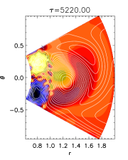
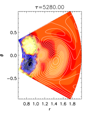
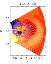
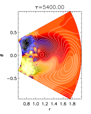
Figure 1: Time series of formation of a plasmoid ejection in spherical coordinates. Contours of $r\sin{\theta}\langle A_{\phi}\rangle_{\phi}$ are shown together with a color-scale representation of $\langle B_{\phi}\rangle_{\phi}$; dark blue stands for negative and red for positive values. The contours of $r\sin{\theta}\langle A_{\phi}\rangle_{{\phi}}$ correspond to field lines of $\langle\mbox{\boldmath$B$}{}\rangle_{\phi}$ in the $r\theta$ plane. The dotted horizontal lines show the location of the surface at $r=1\,R_{\odot}$.

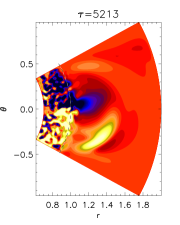
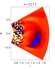
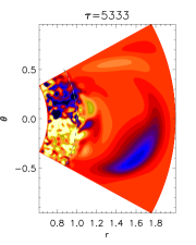
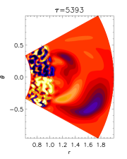
Figure 2: Times series of what looks a bit like coronal ejections in spherical coordinates. The normalized current helicity $\langle\mbox{\boldmath$J$}{}\cdot\mbox{\boldmath$B$}{}\rangle_{\phi}/\overline{\langle\mbox{\boldmath$B$}{}^{2}\rangle_{\phi}}$ is shown in a color-scale representation for different times; dark blue stands for negative and red for positive values. The dotted horizontal lines show the location of the surface at $r=1\,R_{\odot}$.

Investigating the current helicity, we find a surprising result. In the turbulence zone the $\langle\mbox{\boldmath$J$}{}\cdot\mbox{\boldmath$B$}{}\rangle_{\phi}/\langle\mbox{\boldmath$B$}{}^{2}\rangle_{\phi}$ is negative in the northern hemisphere and positive in south, i.e., has the same sign as the helicity of the external force. Above the surface, for each hemisphere, current helicity with sign opposite to the turbulent layer is ejected in large patches (Fig. 2). These structures correlate with reconnection events of strong magnetic fields. In Rust (1994) such phenomena have been described as magnetic clouds. In order to demonstrate that plasmoid ejection is a recurrent phenomenon, we plot the evolution of the ratio $\langle\mbox{\boldmath$J$}{}\cdot\mbox{\boldmath$B$}{}\rangle_{\phi}/\langle\mbox{\boldmath$B$}{}^{2}\rangle_{\phi}$ versus $\tau$ and $r$ in Fig. 3. We further find that the typical speed of plasmoid ejection is about 0.13 times the rms velocity of the turbulence in the interior region, which corresponds to 0.08 of the Alfvén speed. The time interval between successive ejections is about 100 $\tau$. Note that the ejection of magnetic field and associated reconnection events are fairly regular, but the formation structures such as magnetic clouds are less regular. Note further that the sign of azimuthally averaged current helicity in the outer layer is always opposite to that of the turbulence zone. This is demonstrated in Fig. 4 where we plot time-series of azimuthally averaged current helicity at $r=1.5\,R_{\odot}$. For the northern hemisphere the current helicity (solid black line) and the accumulated mean (solid red line) show positive values and for the southern hemisphere (dotted lines) negative values. This suggests that, even though the plasmoids observed in our simulations are shedding small-scale current helicity of opposite sign to that of the large-scale current helicity inside the turbulence zone, outside the turbulence zone the sign of large-scale current helicity has reversed and is now the same as that of the small-scale helicity. This may be explained by the action of turbulent magnetic diffusion on the magnetic field; see e.g., Brandenburg, Candelaresi, & Chatterjee (2009).

In summary, it turns out that twisted magnetic fields generated by the helical dynamo beneath a spherical surface are able to produce flux emergence in ways that are reminiscent of that found in the Sun. We find phenomena that can be interpreted as recurrent plasmoid ejections, which then lead to magnetic clouds further out. A promising extension of this work would be to include a Parker–like wind that turns into a supersonic flow at sufficiently large radii.

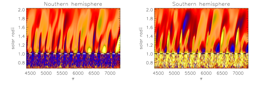
Figure 3: Dependence of $\langle{\mbox{\boldmath$J$}{}\cdot\mbox{\boldmath$B$}{}}_{\phi}\,\theta\rangle/\overline{\langle\mbox{\boldmath$B$}{}^{2}\rangle_{\phi\theta}}$ versus time $\tau$ and radius $r$ in terms of the solar radius $R_{\odot}$. The left penal show a thin band in $\theta$ in the northern hemisphere, the right one a thin band in $\theta$ in the southern hemisphere, both are averaged over 20^∘–28^∘ latitude. Dark blue stands for negative and red for positive values. The dotted horizontal lines show the location of the surface at $r=1\,R_{\odot}$.

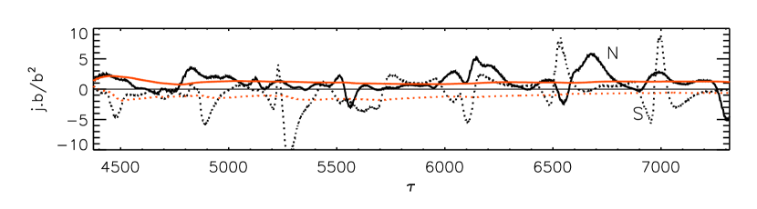
Figure 4: Dependence of $\langle\mbox{\boldmath$J$}{}\cdot\mbox{\boldmath$B$}{}\rangle_{\phi}/\overline{\langle\mbox{\boldmath$B$}{}^{2}\rangle_{\phi}}$ versus time $\tau$ for a radius of $r=1.5\,R_{\odot}$ at $\pm 28^{\circ}$ latitude in arbitrary units. The solid lines stand for the northern hemisphere and the dotted for the southern hemisphere. The red colored lines represent accumulated means for each hemisphere.

References

- [] Brandenburg, A., Candelaresi, S., & Chatterjee, P. 2009, MNRAS, 398, 1414
- [] Käpylä, P. J., Korpi, M. J., & Brandenburg, A. 2008, A&A, 491, 353
- [] Mitra, D., Tavakol,R., Käpylä, P. J., & Brandenburg, A. 2010, ApJ, 719, L1-L4.
- [] Mitra, D., Tavakol, R., Brandenburg, A., & Moss, D. 2009, ApJ, 697, 923
- [] Nordlund, Å., Brandenburg, A., Jennings, R. L., et al. 1992, ApJ, 392, 647
- [] Rust, D. M. 1994, Geophys. Res. Lett., 21, 241
- [] Tobias, S. M., Brummell, N. H., Clune, T. L., & Toomre, J. 1998, ApJ, 502, L177
- [] Warnecke, J., & Brandenburg, A. 2010, A&A, 523, A19