Field theory description of neutrino oscillations

Abstract

We review various field theory approaches to the description of neutrino oscillations in vacuum and external fields. First we discuss a relativistic quantum mechanics based approach which involves the temporal evolution of massive neutrinos. To describe the dynamics of the neutrinos system we use exact solutions of wave equations in presence of an external field. It allows one to exactly take into account both the characteristics of neutrinos and the properties of an external field. In particular, we examine flavor oscillations an vacuum and in background matter as well as spin flavor oscillations in matter under the influence of an external electromagnetic field. Moreover we consider the situation of hypothetical nonstandard neutrino interactions with background fermions. In the case of ultrarelativistic particles we reproduce an effective Hamiltonian which is used in the standard quantum mechanical approach for the description of neutrino oscillations. The corrections to the quantum mechanical Hamiltonian are also discussed. Note that within the relativistic quantum mechanics method one can study the evolution of both Dirac and Majorana neutrinos. We also consider several applications of this formalism to the description of oscillations of astrophysical neutrinos emitted by a supernova and compare the behavior of Dirac and Majorana neutrinos. Then we study a spatial evolution of mixed massive neutrinos emitted by classical sources. This method seems to be more realistic since it predicts neutrino oscillations in space. Besides oscillations among different neutrino flavors, we also study transitions between particle and antiparticle states. Finally we use the quantum field theory method, which involves virtual neutrinos propagating between production and detection points, to describe particle-antiparticle transitions of Majorana neutrinos in presence of background matter.

I Introduction

Neutrino physics is one of the most rapidly developing area of high energy physics especially after the great success in experimental studies of neutrino properties. In the first place we should mention the investigation of astrophysical neutrinos since they play an important role in the evolution of various astronomical objects like stars, supernovas, quasars etc. In the course of recent experiments for the detection of solar neutrinos Abe10 it was revealed that transitions between different neutrino flavors, neutrino oscillations, are the most plausible theoretical explanation of the solar neutrinos deficit BahPin04 . Flavor oscillations were also observed in the experimental studies of atmospheric neutrinos Wen10 . It is worth noticing that there are numerous attempts to detect neutrinos from outside the solar system (see, e.g., Ref. Abb10 ), however, presently only SN1987A supernova neutrinos were observed Hir87 .

Besides natural sources, one can use neutrinos produced by an accelerator or a nuclear reactor to study oscillations of these particles Gan10 . In this case we control the flavor content of both initial and final fluxes, i.e. it is the best strategy to examine neutrino oscillations. Besides the studies of neutrino oscillations, some accelerator based experiments are dedicated to the investigation of neutrino interactions (see, e.g., Ref. Kur10 ).

The existence of neutrino oscillations is a direct indication to the facts that neutrinos are massive particles and there is a mixing between different neutrino generations. There are multiple theoretical mechanisms to generate masses and mixing of neutrinos MohSmi06 to fit the data of the aforementioned neutrino oscillations experiments.

It was found that besides the possibility of flavor conversions in vacuum, various external fields, like interaction with background matter Wol78 or with an external magnetic field Cis71 , can significantly influence neutrino oscillations. For example, the resonant enhancement of neutrino oscillations in matter, Mikheev-Smirnov-Wolfenstein (MSW) effect, plays an important role in the solution of the solar neutrino problem HolSmi03 . It should be noted that the standard model of electroweak interactions does not imply the mixing between different neutrino flavors when particles propagate in background matter. However the possibility of nonstandard neutrino interactions, which can cause transitions between neutrino flavors even at the absence of vacuum mixing, was recently discussed Big09 .

Since neutrinos are unlikely to have a nonzero electric charge IgnJos95 , the interaction with an external electromagnetic field may be implemented due to the presence of anomalous magnetic moments. Note that, unlike an electron which has a vacuum magnetic moment, electromagnetic moments of a neutrino always arise from the loop corrections. The contributions to neutrino electromagnetic moments in various extensions of the standard model are reviewed in Ref. GiuStu09 .

It should be noted that neutrino electromagnetic properties have rather complicated structure. First, in the system of mixed neutrinos there can be both diagonal and transition magnetic moments. In presence of an external electromagnetic field the former are responsible for the helicity flip within one neutrino generation and the latter cause the change of neutrino flavor (spin flavor oscillations). Second, electromagnetic properties of Dirac and Majorana neutrinos are completely different. In general case Dirac neutrinos can have all kinds of magnetic moments, whereas Majorana neutrinos possess only transition magnetic moments which are antisymmetric in neutrino flavors FukYan03p461 . Nowadays there is no universally recognized experimental confirmation of the nature of neutrinos AviEllEng08 . Thus it is important to study the evolution of both Dirac and Majorana neutrinos in an external electromagnetic field.

The indication to the Majorana nature of neutrinos should be experimental confirmation of the existence of neutrinoless double $\beta$-decay ($0\nu 2\beta$), which is the manifestation of oscillations between neutrinos and antineutrinos Bil10 . This kind of transitions is possible only if neutrinos are Majorana particles. Despite numerous attempts to detect ($0\nu 2\beta$)-decay in a laboratory were made Arg09 , no confirmed events are known presently.

The great variety of evidences of neutrino oscillations requires a rigorous theoretical explanation of this phenomenon. The conventional approach to the description of neutrino oscillations is based on the quantum mechanical evolution of neutrino flavor eigenstates governed by an effective Hamiltonian BilPon78 . This intuitive approach may be easily extended to the description of neutrino oscillations in background matter Wol78 and spin flavor oscillations in an external magnetic field LimMar88 giving one a reasonable description of neutrino oscillations in these external fields.

Neutrinos are supposed to propagate as plane waves in the quantum mechanical approach. However, due to uncertainties in production and detection processes, neutrinos seem to have some distribution of their momenta, i.e. they propagate like wave packets Kay81 . The Gaussian distribution of the neutrino momentum is typically discussed Giu02 . However the actual form of the distribution strongly depends on the production and detection processes (see, e.g., Ref. Dol05 ). The necessity of the wave packets treatment of neutrino oscillations is discussed in Ref. Sto98 . The details of this approach including its extension to the Dirac theory were considered in Ref. BerGuzNis10 .

The attempts to reproduce the quantum mechanical transition probability formula in vacuum were made in Refs. Kob82 ; GiuKimLeeLee93 treating massive neutrinos as virtual particles propagating between production and detection points. Using this quantum field theory method one deals with the observables of charged leptons rather than with the characteristics of mixed neutrinos. The special Gaussian form of the source and detector within this quantum field theory approach was discussed in Ref. IoaPil99 . The analysis of relativistic effects in neutrino oscillations using this approach was made in Ref. NauNau10 .

In Ref. BlaVit95 neutrino flavor oscillations in vacuum are described on the basis of time evolution of the Fock states of flavor neutrinos. The time dependent transition probability formula, obtained within the $S$-matrix approach, was studied in Ref. Wu10 . The quantum mechanics analysis of the neutrino detection process and the possibility to obtain the nonstandard transition probability formulas is considered in Ref. AnaSav10 .

We contributed to the field theoretical description of neutrino oscillations in Refs. Dvo05 ; Dvo06 ; DvoMaa07 ; Dvo08JPCS ; Dvo08JPG ; Dvo09 ; DvoMaa09 ; Dvo10 . We developed an approach based on relativistic quantum mechanics and applied it for the description of neutrino flavor oscillations in vacuum Dvo05 , in background matter Dvo06 ; Dvo08JPCS , and to spin flavor oscillations in an external electromagnetic field DvoMaa07 ; Dvo08JPG ; DvoMaa09 ; Dvo10 . This method is based on the first quantized neutrino wave packets which was also studied in Ref. BerLeo04 to study neutrino oscillations in vacuum and in an external electromagnetic field.

In frames of the relativistic quantum mechanics method we formulate the initial condition problem for the system of flavor neutrinos and study the subsequent time evolution of neutrino wave packets. When we discuss neutrino propagation in an external field, we use an exact solution of the corresponding wave equation in presence of this external field. With help of this method we could reproduce the Schrödinger type evolution equation, which is used in the standard quantum mechanical description of Dirac and Majorana neutrino oscillations, and discuss the correction to the standard approach.

In Ref. Dvo09 we studied neutrino flavor oscillation in vacuum within the external classical sources method. Note that the analogous approach to the description of neutrino oscillations was also discussed in Ref. KieWei98 . Within this approach we studied the spatial evolution of flavor neutrino waves emitted by external classical sources. We could describe the evolution of both Dirac and Majorana neutrinos in vacuum.

In the present work we review our recent achievements in theoretical description of neutrino flavor oscillations. This work is organized as follows. In Secs. II-V we discuss oscillations of Dirac neutrinos in frames of relativistic quantum mechanics method. We start with the description of neutrino flavor oscillations in vacuum (Sec. II). Then we consider oscillations in background matter (Sec. III), where we also study oscillations in case of nonstandard neutrino interactions with matter. In Sec. IV we apply the relativistic quantum mechanics method to the description of spin flavor oscillations of Dirac neutrinos in an external magnetic field. Finally, in Sec. V, we discuss the most general situation of spin flavor oscillations in matter under the influence of an external magnetic field. In Secs. VI and VII we examine applications of the relativistic quantum mechanics method to the description of propagation and oscillations of astrophysical neutrinos in a magnetized envelope after the supernova explosion.

In Secs. VIII and IX we analyze the evolution of massive mixed Majorana neutrinos in vacuum as well as in matter and magnetic field in frames of the relativistic quantum mechanics approach. Besides oscillations among different neutrino flavors we also consider transitions between neutrino and antineutrino states which are allowed if neutrinos are Majorana particles. In Sec. X we apply the general results to the studies of oscillations of astrophysical neutrinos in the supernova envelope supposing that neutrinos are Majorana particles and compare them with the Dirac neutrino case studied in Sec. VI.

Then, in Sec. XI, we formulate an alternative formalism for the description of neutrino flavor oscillations which is based on the mixed massive neutrinos emission by classical sources. We examine the spatial distribution of flavor neutrino wave functions in case of localized sources. Note that vacuum oscillations of both Dirac (Sec. XI.1) and Majorana (Sec. XI.2) neutrinos are studied. When we discuss Majorana neutrinos case, we also consider the possibility of transitions between particles and antiparticles.

Finally, in Sec. XII, we consider the transitions among neutrinos and antineutrinos in frames of the quantum field theory, treating neutrinos as virtual particles propagating between macroscopically separated production and detection points (see also Refs. Kob82 ; GiuKimLeeLee93 ; IoaPil99 ; NauNau10 ). In particular we are interested in the influence of background matter on the oscillations process since this kind of transitions typically happens inside a nucleus (see, e.g., Ref. Bil10 ) and one cannot neglect the presence of dense nuclear matter in neutrino oscillations.

In Sec. XIII we summarize our results. Several technical issues are considered in Appendices A-D in order not to encumber the description of the main results in Secs. II-XII.

II Dirac neutrinos in vacuum

In this section we discuss the evolution of mixed flavor neutrinos in vacuum, i.e. at the absence of external fields, using the relativistic quantum mechanics approach Dvo05 . First we formulate the initial condition problem for the system of flavor neutrinos. We exactly solve this problem and find the time dependent wave functions and the transition probability. We also discuss the validity of the developed formalism.

Without loss of generality we study the situation of only two particles $\nu=(\nu_{\alpha},\nu_{\beta})$, where $\alpha$ and $\beta$ can stay for electron, muon or $\tau$-neutrinos. In various theoretical models (see, e.g., Ref. Moh04 ) bigger number of flavor neutrino fields $N_{\nu}>3$ is proposed. The case of arbitrary number of neutrino fields can be considered in our formalism by straightforward generalization. The Lorentz invariant Lagrangian for this system has the following form:

$$\mathcal{L}=\sum_{\lambda=\alpha,\beta}\bar{\nu}_{\lambda}\mathrm{i}\gamma^{\mu}\partial_{\mu}\nu_{\lambda}-\sum_{\lambda\lambda^{\prime}=\alpha,\beta}m_{\lambda\lambda^{\prime}}\bar{\nu}_{\lambda}\nu_{\lambda^{\prime}},$$ (1)

where $\gamma^{\mu}=(\gamma^{0},\bm{\gamma})$ are Dirac matrices and $(m_{\lambda\lambda^{\prime}})$ is the mass matrix which is not diagonal in the flavor neutrinos basis. The nondiagonal elements of this matrix $m_{\alpha\beta}=m_{\beta\alpha}$ correspond to the mixing between different neutrino flavors.

To describe the time evolution of the system (1) we formulate the initial condition problem for flavor neutrinos $\nu_{\lambda}$,

$$\nu_{\lambda}(\mathbf{r},t=0)=\nu_{\lambda}^{(0)}(\mathbf{r}),\quad\lambda=\alpha,\beta,$$ (2)

where $\nu_{\lambda}^{(0)}(\mathbf{r})$ are known functions. Eq. (2) means that initial field distributions of flavor neutrinos are known and we will search for their wave functions at subsequent moments of time: $\nu_{\lambda}(\mathbf{r},t>0)$. The situation when only one of the flavor neutrinos, e.g. belonging to the type “$\beta$”, is present initially corresponds to a typical neutrino oscillations experiment: one looks for the initially absent neutrino flavor “$\alpha$” in a beam consisting of neutrinos of the flavor “$\beta$”.

To solve the initial condition problem (2) for the system (1) we introduce the mass eigenstates neutrinos $\psi_{a}$, $a=1,2$,

$$\nu_{\lambda}=\sum_{a=1,2}U_{\lambda a}\psi_{a},$$ (3)

where the matrix $(U_{\lambda a})$ is chosen in such a way to diagonalize the mass matrix $(m_{\lambda\lambda^{\prime}})$. The eigenvalues of the matrix $(m_{\lambda\lambda^{\prime}})$, which are real and positive, have the meaning of the masses of the fields $\psi_{a}$. We define them as $m_{a}$.

The Lagrangian formulated in terms of the flavor neutrino fields does not provide any information about the nature of neutrinos, i.e. whether neutrinos are Dirac or Majorana particles, since in general case it is written using the two component left and right handed spinors Kob80 ; SchVal80 . Only when we introduce the mass eigenstates and analyze the structure of resulting mass matrices, we can reveal the nature of neutrinos. We suppose that in our case the fields $\psi_{a}$ are Dirac particles.

For the case of only two neutrinos system the mixing matrix $(U_{\lambda a})$ in Eq. (3) has the form,

$$(U_{\lambda a})=\begin{pmatrix}\cos\theta&-\sin\theta\\ \sin\theta&\cos\theta\ \end{pmatrix},$$ (4)

where $\theta$ is the vacuum mixing angle.

The Lagrangian (1) expressed in terms of the fields $\psi_{a}$ reads

$$\mathcal{L}=\sum_{a=1,2}\bar{\psi}_{a}(\mathrm{i}\gamma^{\mu}\partial_{\mu}-m_{a})\psi_{a}.$$ (5)

The Lagrangian (5) should be supplied with the initial condition,

$$\psi_{a}(\mathbf{r},t=0)=\psi_{a}^{(0)}(\mathbf{r}),\quad\psi_{a}^{(0)}=(U_{a\lambda}^{-1})\nu_{\lambda}^{(0)},$$ (6)

which follows from Eqs. (2) and (3).

The Dirac equations,

$$\mathrm{i}\dot{\psi}_{a}=(\bm{\alpha}\mathbf{p}+\beta m_{a})\psi_{a},$$ (7)

which result from the Lagrangian (5), reveal that the fields $\psi_{a}$ decouple. In Eq. (7) we use the standard definitions for Dirac matrices $\bm{\alpha}=\gamma^{0}\bm{\gamma}$ and $\beta=\gamma^{0}$. The solution of Eq. (7) can be found in the following way:

$$\psi_{a}(\mathbf{r},t)= \int\frac{\mathrm{d}^{3}\mathbf{p}}{(2\pi)^{3/2}}e^{\mathrm{i}\mathbf{p}\mathbf{r}}$$

$$\times\sum_{\zeta=\pm 1}\left[a_{a}^{(\zeta)}u_{a}^{(\zeta)}e^{-\mathrm{i}E_{a}t}+b_{a}^{(\zeta)}v_{a}^{(\zeta)}e^{\mathrm{i}E_{a}t}\right],$$ (8)

where $E_{a}=\sqrt{|\mathbf{p}|^{2}+m_{a}^{2}}$ is the energy of a massive neutrino in vacuum, $\zeta=\pm 1$ is the helicity of massive neutrinos, and $u_{a}^{(\zeta)}$ and $v_{a}^{(\zeta)}$ are the basis spinors corresponding to a definite helicity.

In the relativistic quantum mechanics approach to the description of neutrinos evolution Dvo05 the coefficients $a_{a}^{(\zeta)}$ and $b_{a}^{(\zeta)}$ are $c$-number quantities rather than operators acting in the Fock space. Our task is to find these coefficients. Since the fields $\psi_{a}$ are independent, the values of the coefficients $a_{a}^{(\zeta)}$ and $b_{a}^{(\zeta)}$ depends only on the initial condition (6).

Using the orthonormality of the basis spinors,

$$u_{a}^{(\zeta^{\prime}){\dagger}}u_{a}^{(\zeta)}=v_{a}^{(\zeta^{\prime}){\dagger}}v_{a}^{(\zeta)}=\delta_{\zeta^{\prime}\zeta},\quad u_{a}^{(\zeta^{\prime}){\dagger}}v_{a}^{(\zeta)}=0,$$ (9)

we find the coefficients $a_{a}^{(\zeta)}$ and $b_{a}^{(\zeta)}$ in the form,

$$a_{a}^{(\zeta)}= \frac{1}{(2\pi)^{3/2}}u_{a}^{(\zeta){\dagger}}\psi_{a}^{(0)}(\mathbf{p}),$$

$$b_{a}^{(\zeta)}= \frac{1}{(2\pi)^{3/2}}v_{a}^{(\zeta){\dagger}}\psi_{a}^{(0)}(\mathbf{p}),$$ (10)

where

$$\psi_{a}^{(0)}(\mathbf{p})=\int\mathrm{d}^{3}\mathbf{r}e^{-\mathrm{i}\mathbf{p}\mathbf{r}}\psi_{a}^{(0)}(\mathbf{r}),$$ (11)

is the Fourier transform of the initial condition (6).

With help of Eqs. (II)-(11) we arrive to the expression for the wave function of the neutrino mass eigenstates,

$$\psi_{a}(\mathbf{r},t)=\int\mathrm{d}^{3}\mathbf{r}^{\prime}S_{a}(\mathbf{r}^{\prime}-\mathbf{r},t)(-\mathrm{i}\gamma^{0})\psi_{a}^{(0)}(\mathbf{r}^{\prime}),$$ (12)

where

$$S_{a}(\mathbf{r},t)=(\mathrm{i}\gamma^{\mu}\partial_{\mu}+m_{a})D_{a}(\mathbf{r},t),$$ (13)

is the Pauli-Jourdan function for a spinor particle and

$$D_{a}(\mathbf{r},t)=\int\frac{\mathrm{d}^{3}\mathbf{p}}{(2\pi)^{3}}e^{\mathrm{i}\mathbf{p}\mathbf{r}}\frac{\sin E_{a}t}{E_{a}},$$ (14)

is the Pauli-Jourdan function for a scalar particle.

It is convenient to rewrite Eq. (12) in the form,

$$\psi_{a}(\mathbf{r},t)=\int\frac{\mathrm{d}^{3}\mathbf{p}}{(2\pi)^{3}}e^{\mathrm{i}\mathbf{p}\mathbf{r}}S_{a}(-\mathbf{p},t)(-\mathrm{i}\gamma^{0})\psi_{a}^{(0)}(\mathbf{p}),$$ (15)

where

$$S_{a}(-\mathbf{p},t)= \sum_{\zeta=\pm 1}\big{(}u_{a}^{(\zeta)}\otimes u_{a}^{(\zeta){\dagger}}e^{-\mathrm{i}E_{a}t}$$

$$+v_{a}^{(\zeta)}\otimes v_{a}^{(\zeta){\dagger}}e^{\mathrm{i}E_{a}t}\big{)}(\mathrm{i}\gamma^{0})$$

$$=\left[\cos E_{a}t-\mathrm{i}\frac{\sin E_{a}t}{E_{a}}(\bm{\alpha}\mathbf{p}+\beta m_{a})\right]$$

$$\times(\mathrm{i}\gamma^{0}),$$ (16)

is the Fourier transform of the Pauli-Jourdan function (13). To derive Eq. (II) we use the summation over the helicity index formulas BogShi80 ,

$$\sum_{\zeta=\pm 1}u_{a}^{(\zeta)}\otimes u_{a}^{(\zeta){\dagger}}= \frac{1}{2}+\frac{1}{2E_{a}}(\bm{\alpha}\mathbf{p}+\beta m_{a}),$$

$$\sum_{\zeta=\pm 1}v_{a}^{(\zeta)}\otimes v_{a}^{(\zeta){\dagger}}= \frac{1}{2}-\frac{1}{2E_{a}}(\bm{\alpha}\mathbf{p}+\beta m_{a}),$$ (17)

which are consistent with the normalization of the basis spinors (9).

Now let us specify the initial condition (2). We suggest that initially very broad wave packet is present, i.e. the coordinate dependence of the wave functions $\nu_{\lambda}^{(0)}(\mathbf{r})$ is close to a plane wave corresponding to the initial momentum $\mathbf{k}$. Moreover we choose the situation when only one flavor neutrino is present,

$$\nu_{\alpha}^{(0)}(\mathbf{r})=0,\quad\nu_{\beta}^{(0)}(\mathbf{r})=e^{\mathrm{i}\mathbf{k}\mathbf{r}}\nu_{\beta}^{(0)}(\mathbf{k}),$$ (18)

where $\nu_{\alpha}^{(0)}(\mathbf{k})$ is the coordinate independent normalization spinor, $|\nu_{\beta}^{(0)}(\mathbf{k})|^{2}=1$.

Using Eqs. (3), (4), and (14)-(18) we obtain the wave function of the initially absent flavor neutrino $\nu_{\alpha}$ as

$$\nu_{\alpha}(\mathbf{r},t)= e^{\mathrm{i}\mathbf{k}\mathbf{r}}\sin\theta\cos\theta\bigg{\{}\cos E_{1}t-\cos E_{2}t$$

$$-\mathrm{i}\frac{\sin E_{1}t}{E_{1}}(\bm{\alpha}\mathbf{k}+\beta m_{1})$$

$$+\mathrm{i}\frac{\sin E_{2}t}{E_{2}}(\bm{\alpha}\mathbf{k}+\beta m_{2})\bigg{\}}\nu_{\beta}^{(0)}(\mathbf{k}),$$ (19)

where the energies are the functions of the initial momentum, $E_{a}=\sqrt{|\mathbf{k}|^{2}+m_{a}^{2}}$.

With help of Eq. (II) we get the transition probability $P_{\nu_{\beta}\to\nu_{\alpha}}(t)=|\nu_{\alpha}(\mathbf{r},t)|^{2}$ as

$$P_{\nu_{\beta}\to\nu_{\alpha}}(t)= \sin^{2}(2\theta)\bigg{[}\sin^{2}(\Phi t)-\sin(\Phi t)\cos(\sigma t)$$

$$\times\frac{1}{2}\left(\frac{m_{1}^{2}}{k^{2}}\sin E_{1}t-\frac{m_{2}^{2}}{k^{2}}\sin E_{2}t\right)\bigg{]}$$

$$+\mathcal{O}\left(\frac{m_{a}^{4}}{k^{4}}\right),$$ (20)

where

$$\Phi= \frac{E_{1}-E_{2}}{2}\approx\frac{\delta m^{2}}{4k}+\dotsb,$$

$$\sigma= \frac{E_{1}+E_{2}}{2}\approx k+\frac{m_{1}^{2}+m_{2}^{2}}{4k}+\dotsb,$$ (21)

and $\delta m^{2}=m_{1}^{2}-m_{2}^{2}$. The quantity $\Phi$ has the meaning of the phase of neutrino oscillations in vacuum. Note that the coordinate dependence is washed out from Eq. (II) since we study a very broad initial wave packet.

In the untrarelativistic limit (II) the main term in Eq. (II) resembles the usual transition probability for neutrino oscillations in vacuum. The correction to the main result is suppressed by the factor $m_{a}^{2}/k^{2}\ll 1$. Using Eq. (II) we can represent Eq. (II) in the following form:

$$P_{\nu_{\beta}\to\nu_{\alpha}}(t)= \sin^{2}(2\theta)\bigg{[}\sin^{2}\left(\frac{\delta m^{2}}{4k}t\right)-\frac{\delta m^{2}}{4k^{2}}$$

$$\times\sin\left(\frac{\delta m^{2}}{4k}t\right)\sin(2kt)\bigg{]}+\dotsb,$$ (22)

where we drop small terms $\sim m_{a}^{4}/k^{4}$.

Now the leading term in Eq. (II) reproduces the well known transition probability for neutrino oscillations in vacuum derived in frames of the quantum mechanical approach GriPon69 . The correction to the leading term, which is a rapidly oscillating function on the frequency $\sim k$, was first studied in Ref. BlaVit95 in frames of the quantum field theory approach to neutrino oscillations. We obtained analogous result using the relativistic quantum mechanics method (see also Ref. Dvo05 ). This correction to the leading term in the transition probability results from the accurate account of the Lorentz invariance.

Note that Eq. (II) is invariant under the $m_{1}\leftrightarrow m_{2}$ transformation. It means that one cannot obtain the information about neutrino mass hierarchy studying neutrino oscillations in vacuum even taking into account the correction to the leading term in the transition probability.

Now let us discuss the possibility of initial conditions which differ from the plane wave (18). If the initial wave function is localized in a spatial region with a typical size $L_{0}$ and we measure a signal in the wave zone $|\mathbf{r}|\gg L_{0}$, the dependence on the particle masses $m_{a}$ is washed out from the Pauli-Jourdan functions (14) and (13) (see Refs. Dvo05 ; MorFes53 ). Thus neutrinos with spatially localized initial wave packets evolve in the wave zone like massless particles, which are known not to reveal flavor oscillations. Therefore the initial wave packet should be sufficiently broad.

III Dirac neutrinos in background matter

In this section we use the formalism developed in Sec. II to study the evolution of the system of mixed flavor neutrinos $\nu=(\nu_{\alpha},\nu_{\beta})$ in background matter Dvo06 ; Dvo08JPCS . We formulate the initial condition problem for this system and solve it for ultrarelativistic neutrinos. The case of the standard model neutrino interactions is studied in details. Then we also analyze the dynamics of neutrino oscillations in presence of the nonstandard interactions which mix neutrino flavors.

The neutrino interaction with matter can be represented in the form of an external axial-vector field $f_{\lambda\lambda^{\prime}}^{\mu}$ DvoStu02 ; LobStu01 . As in Sec. II, we start from the Lorentz invariant Lagrangian,

$$\mathcal{L}= \sum_{\lambda=\alpha,\beta}\bar{\nu}_{\lambda}\mathrm{i}\gamma^{\mu}\partial_{\mu}\nu_{\lambda}$$

$$-\sum_{\lambda,\lambda^{\prime}=\alpha,\beta}\bar{\nu}_{\lambda}\left(m_{\lambda\lambda^{\prime}}+f_{\lambda\lambda^{\prime}}^{\mu}\gamma_{\mu}^{\mathrm{L}}\right)\nu_{\lambda^{\prime}},$$ (23)

where $\gamma_{\mu}^{\mathrm{L}}=\gamma_{\mu}(1-\gamma^{5})/2$, $\gamma^{5}=\mathrm{i}\gamma^{0}\gamma^{1}\gamma^{2}\gamma^{3}$, and keep the same notation for the mass matrix as in Sec. II.

Note that in general case the axial vector field $f_{\lambda\lambda^{\prime}}^{\mu}$ can be nondiagonal in the neutrino flavor basis. The appearance of nondiagonal elements $(f_{\alpha\beta}^{\mu})$ of this matrix is the indication to the presence of nonstandard neutrino interactions which mix neutrino flavors since in the standard model of electroweak interactions only diagonal elements of this matrix can appear. The time component of diagonal elements of this matrix, $f_{\lambda\lambda}^{0}$, is proportional to the density of background matter and spatial component, $\mathbf{f}_{\lambda\lambda}$, to the mean velocity and polarization of background fermions. The details of the averaging over the background fermions are presented in Ref. LobStu01

To describe the evolution of the system (III) we formulate the initial condition problem for flavor neutrinos, with the initial wave functions having an analogous form as in Eq. (2). To solve the initial condition problem we introduce the set of neutrino mass eigenstates $\psi_{a}$ [see Eqs. (3) and (4)] to diagonalize the mass matrix $(m_{\lambda\lambda^{\prime}})$. As in Sec. II we suggest that mass eigenstates $\psi_{a}$ are Dirac particles.

The Lagrangian (III) expressed in terms of the fields $\psi_{a}$ has the form,

$$\mathcal{L}=\sum_{a=1,2}\bar{\psi}_{a}(\mathrm{i}\gamma^{\mu}\partial_{\mu}-m_{a})\psi_{a}-\sum_{a,b=1,2}g_{ab}^{\mu}\bar{\psi}_{a}\gamma_{\mu}^{\mathrm{L}}\psi_{b},$$ (24)

where

$$(g_{ab}^{\mu})=U^{\dagger}(f_{\lambda\lambda^{\prime}}^{\mu})U=\begin{pmatrix}g_{1}^{\mu}&g^{\mu}\\ g^{\mu}&g_{2}^{\mu}\ \end{pmatrix},$$ (25)

is the external axial-vector field expressed in the mass eigenstates basis.

One can derive Dirac equations for the neutrino mass eigenstates,

$$\mathrm{i}\dot{\psi}_{a}= \mathcal{H}_{a}\psi_{a}+\mathcal{V}\psi_{b},\quad a,b=1,2,\quad a\neq b,$$

$$\mathcal{H}_{a}= \bm{\alpha}\mathbf{p}+\beta m_{a}+\beta\gamma_{\mu}^{\mathrm{L}}g_{a}^{\mu},\quad\mathcal{V}=\beta\gamma_{\mu}^{\mathrm{L}}g^{\mu},$$ (26)

directly from the Lagrangian (24). It should be noted that Dirac equations for different neutrino mass eigenstates are coupled because of the presence of the interaction $\mathcal{V}$. Studying an exact solution of the Dirac equation for a massive neutrino in background matter we can exactly take into account the contribution of the term $\beta\gamma_{\mu}^{\mathrm{L}}g_{a}^{\mu}$ into the dynamics of a particle. On the contrary, the term proportional to $\mathcal{V}$, which mixes different mass eigenstates, should be studied perturbatively. Nevertheless one can account for all terms in the perturbative expansion for ultrarelativistic neutrinos.

We will study the case of nonmoving and unpolarized matter which corresponds to $\mathbf{g}_{ab}=0$. The matrix $(g_{ab}^{\mu})$ has only time component now,

$$(g_{ab})\equiv(g_{ab}^{0})=\begin{pmatrix}g_{1}&g\\ g&g_{2}\ \end{pmatrix},$$ (27)

where we introduce the new notations, $g_{a}\equiv g_{aa}^{0}$ and $g\equiv g_{12}^{0}=g_{21}^{0}$. If the background matter is nonmoving and unpolarized, the Hamiltonian $\mathcal{H}_{a}$ commutes with the helicity operator $(\bm{\Sigma}\mathbf{p})/|\mathbf{p}|$, where $\bm{\Sigma}=\gamma^{0}\gamma^{5}\bm{\gamma}$, and we can classify the states of massive neutrinos with help of the eigenvalues of the helicity operator $\zeta=\pm 1$.

The general solution of Eq. (III) can be presented in the following way:

$$\psi_{a}(\mathbf{r},t)= e^{-\mathrm{i}g_{a}t/2}\int\frac{\mathrm{d}^{3}\mathbf{p}}{(2\pi)^{3/2}}e^{\mathrm{i}\mathbf{p}\mathbf{r}}$$

$$\times\sum_{\zeta=\pm 1}\big{[}a_{a}^{(\zeta)}(t)u_{a}^{(\zeta)}\exp{(-\mathrm{i}E_{a}^{(\zeta)}t)}$$

$$+b_{a}^{(\zeta)}(t)v_{a}^{(\zeta)}\exp{(+\mathrm{i}E_{a}^{(\zeta)}t)}\big{]},$$ (28)

where $a_{a}^{(\zeta)}$ and $b_{a}^{(\zeta)}$ are the undetermined nonoperator coefficients [see Eq. (II)], which are, however, time dependent now because of the presence of the term $\mathcal{V}$ in Eq. (III).

The energy spectrum $E_{a}^{(\zeta)}$ in Eq. (III) was found in Ref. StuTer05 ,

$$E_{a}^{(\zeta)}=\sqrt{\left(|\mathbf{p}|-\zeta g_{a}/2\right)^{2}+m_{a}^{2}},$$ (29)

for the case of nonmoving and unpolarized neutrinos. The basis spinors $u_{a}^{(\zeta)}$ and $v_{a}^{(\zeta)}$ in Eq. (III) are the eigenvectors of the helicity operator $(\bf{\Sigma}\mathbf{p})/|\mathbf{p}|$, with the eigenvalues $\zeta$. As an example, we present here the basis spinors which correspond to an ultrarelativistic particle propagating along the $z$-axis,

$$u^{-{}}= \frac{1}{\sqrt{2}}\begin{pmatrix}0\\ -1\\ 0\\ 1\ \end{pmatrix},\quad u^{+{}}=\frac{1}{\sqrt{2}}\begin{pmatrix}1\\ 0\\ 1\\ 0\ \end{pmatrix},$$

$$v^{-{}}= \frac{1}{\sqrt{2}}\begin{pmatrix}0\\ 1\\ 0\\ 1\ \end{pmatrix}\quad v^{+{}}=\frac{1}{\sqrt{2}}\begin{pmatrix}1\\ 0\\ -1\\ 0\ \end{pmatrix},$$ (30)

where we omit the subscript “$a$” since we neglect the neutrino mass in Eq. (III). Basis spinors corresponding to arbitrary energies were also found in the explicit form in Ref. StuTer05 .

Now we should specify the initial condition. We can choose it as in Eq. (18), with $\mathbf{k}=(0,0,k)$ and $k\gg m_{a}$. It is also convenient to take $\nu_{\beta}^{(0)}=u^{-{}}$ [see Eq. (III)]. Such an initial wave function corresponds to a neutrino propagating along the $z$-axis, with the spin directed opposite to the particle momentum, i.e. it describes a left polarized neutrino.

If we put the ansatz (III) in the wave equations (III), we get the following ordinary differential equations for the functions $a_{a}^{(\zeta)}(t)$ and $b_{a}^{(\zeta)}(t)$:

$$\mathrm{i}\dot{a}_{a}^{(\zeta)}= e^{\mathrm{i}(g_{a}-g_{b})t/2}\exp\left(\mathrm{i}E_{a}^{(\zeta)}t\right)u^{(\zeta){\dagger}}\mathcal{V}$$

$$\times\sum_{\zeta^{\prime}=\pm 1}\Big{[}a_{b}^{(\zeta^{\prime})}u^{(\zeta^{\prime})}\exp\left(-\mathrm{i}E_{b}^{(\zeta^{\prime})}t\right)$$

$$+b_{b}^{(\zeta^{\prime})}v^{(\zeta^{\prime})}\exp\left(\mathrm{i}E_{b}^{(\zeta^{\prime})}t\right)\Big{]},$$

$$\mathrm{i}\dot{b}_{a}^{(\zeta)}= e^{\mathrm{i}(g_{a}-g_{b})t/2}\exp\left(-\mathrm{i}E_{a}^{(\zeta)}t\right)v^{(\zeta){\dagger}}\mathcal{V}$$

$$\times\sum_{\zeta^{\prime}=\pm 1}\Big{[}a_{b}^{(\zeta^{\prime})}u^{(\zeta^{\prime})}\exp\left(-\mathrm{i}E_{b}^{(\zeta^{\prime})}t\right)$$

$$+b_{b}^{(\zeta^{\prime})}v^{(\zeta^{\prime})}\exp\left(\mathrm{i}E_{b}^{(\zeta^{\prime})}t\right)\Big{]}.$$ (31)

To obtain Eq. (III) we use the orthonormality of the basis spinors (III) [see Eq. (9)]. We should supply the Eq. (III) with the initial condition,

$$a_{1}^{(\zeta)}(0)= \frac{\sin\theta}{(2\pi)^{3/2}}u^{(\zeta){\dagger}}\nu_{\beta}^{(0)},$$

$$a_{2}^{(\zeta)}(0)= \frac{\cos\theta}{(2\pi)^{3/2}}u^{(\zeta){\dagger}}\nu_{\beta}^{(0)},$$ (32)

that result from Eqs. (6) and (III). If we study an arbitrary wave packet initial condition rather than the plane wave distribution for $\nu_{\beta}^{(0)}(\mathbf{r})$ (18), we have to replace $\nu_{\beta}^{(0)}$ in Eq. (III) with the Fourier transform of the initial wave function $\nu_{\beta}^{(0)}(\mathbf{r})$.

Taking into account the fact that $\langle u^{(\zeta)}|\mathcal{V}|v^{(\zeta^{\prime})}\rangle=0$, we get that equations for $a_{a}^{(\zeta)}(t)$ and $b_{a}^{(\zeta)}(t)$ decouple, i.e. the interaction $\mathcal{V}$ does not mix positive and negative energy eigenstates. In the following we will consider the evolution of only $a_{a}^{(\zeta)}(t)$ since the dynamics of $b_{a}^{(\zeta)}(t)$ is studied analogously.

The only nonzero matrix elements of the potential $\mathcal{V}$ in Eq. (III) are $\langle u^{-{}}|\mathcal{V}|u^{-}\rangle=\langle v^{+{}}|\mathcal{V}|v^{+{}}\rangle=g$, which result from Eq. (III). Finally Eq. (III) are reduced to the ordinary differential equations only for the functions $a^{-{}}_{a}(t)$,

$$\mathrm{i}\dot{a}_{a}^{-{}}= a_{b}^{-{}}g\exp{[\mathrm{i}\{E_{a}^{-{}}-E_{b}^{-{}}+(g_{a}-g_{b})/2\}t]},$$

$$a,b=1,2,\quad a\neq b.$$ (33)

It follows from Eq. (III) that equations for the functions $a_{a}^{-{}}$ and $a_{a}^{+{}}$ (not shown here), decouple since the interaction with background matter conserves the particle helicity and we have chosen the initial condition corresponding to a left polarized particle. Indeed one can obtain from Eq. (III) that the functions $a_{a}^{+{}}(t)$ are equal to zero at $t=0$.

The solution of Eq. (III) can be expressed in the form (see Appendix A),

$$a_{1}^{-{}}(t)= Fa_{1}^{-{}}(0)+Ga_{2}^{-{}}(0),$$

$$a_{2}^{-{}}(t)= F^{*{}}a_{2}^{-{}}(0)-G^{*{}}a_{1}^{-{}}(0),$$

$$F= \left[\cos\Omega_{-{}}t-\mathrm{i}\frac{\omega_{-{}}}{2\Omega_{-{}}}\sin\Omega t\right]\exp{(\mathrm{i}\omega_{-{}}t/2)},$$

$$G= -\mathrm{i}\frac{g}{\Omega_{-{}}}\sin\Omega_{-{}}t\exp{(\mathrm{i}\omega_{-{}}t/2)},$$ (34)

where $\Omega_{-{}}=\sqrt{g^{2}+(\omega_{-{}}/2)^{2}}$ and $\omega_{-{}}=E_{1}^{-{}}-E_{2}^{-{}}+(g_{1}-g_{2})/2$.

Using the identity $\left(v^{+{}}\otimes v^{+{}{\dagger}}\right)\nu^{(0)}_{\beta}=0$ [see Eq. (III)] as well as Eqs. (3), (4), (III), and (III) we arrive to the wave function of the flavor neutrino $\nu_{\alpha}$,

$$\nu_{\alpha}(z,t)= -\mathrm{i}\exp{(-\mathrm{i}\sigma_{-{}}t+\mathrm{i}kz)}\frac{\sin\Omega_{-{}}t}{\Omega_{-{}}}$$

$$\times[g\cos 2\theta+(\omega_{-{}}/2)\sin 2\theta]\nu^{(0)}_{\beta}$$

$$+\mathcal{O}\left(\frac{m_{a}}{k}\right),$$ (35)

where $\sigma_{-{}}=(E_{1}^{-{}}+E_{2}^{-{}})/2+(g_{1}+g_{2})/2$. Note that Eq. (III) is the most general one which takes into account the nonstandard interactions of relativistic neutrinos with nonmoving and unpolarized matter of arbitrary density.

Now let us discuss the standard model neutrino interactions with background matter. In this case the matrix $(f_{\lambda\lambda^{\prime}}^{\mu})$ is diagonal: $f_{\lambda\lambda^{\prime}}^{\mu}=f_{\lambda}^{\mu}\delta_{\lambda\lambda^{\prime}}$. Since we study the nonmoving and unpolarized matter the spatial components of the four vector $f_{\lambda}^{\mu}$ are equal zero. If we study the matter composed of electrons, neutrons and protons, the zero-th component $f_{\lambda}^{0}\equiv f_{\lambda}$ is (see, e.g., Ref. DvoStu02 )

$$f_{\lambda}= \sqrt{2}G_{\mathrm{F}}\sum_{f=e,p,n}n_{f}q_{f}^{(\lambda)},$$

$$q_{f}^{(\lambda)}= \left(I^{(f)}_{3\mathrm{L}}-2Q^{(f)}\sin^{2}\theta_{W}+\delta_{fe}\delta_{\lambda\nu_{e}}\right),$$ (36)

where $n_{f}$ is the number density of background particles, $I^{(f)}_{3\mathrm{L}}$ is the third isospin component of the matter fermion $f$, $Q^{(f)}$ is its electric charge, $\theta_{W}$ is the Weinberg angle and $G_{\mathrm{F}}$ is the Fermi constant.

Using Eqs. (4), (25), and (27) and we get that matrix $(g_{ab})$ has the form,

$$(g_{ab})=\\ \begin{pmatrix}f_{\alpha}\cos^{2}\theta+f_{\beta}\sin^{2}\theta&\sin 2\theta\Delta V_{\mathrm{eff}}/2\\ \sin 2\theta\Delta V_{\mathrm{eff}}/2&f_{\alpha}\sin^{2}\theta+f_{\beta}\cos^{2}\theta\ \end{pmatrix},$$ (37)

where $\Delta V_{\mathrm{eff}}=f_{\beta}-f_{\alpha}$ is the difference between the effective potentials of the flavor neutrinos interaction with background matter. With help of Eq. (III) we present $\Delta V_{\mathrm{eff}}$ in the form,

$$\Delta V_{\mathrm{eff}}=\sqrt{2}G_{\mathrm{F}}\times\begin{cases}n_{e},&\text{for $\nu_{e}\to\nu_{\mu,\tau}$},\\ 0,&\text{for $\nu_{\mu,\tau}\to\nu_{\tau,\mu}$},\end{cases}$$ (38)

for various oscillations channels.

In the following we will discuss the low density matter limit, $g_{a}\ll k$, which is fulfilled for all realistic neutrino momenta and densities of background matter. Indeed, even for the background matter in the center of a neutron star where $n_{n}=10^{38}\thinspace\text{cm}^{-3}$, using Eq. (III) we get $g_{a}\sim 10\thinspace\text{eV}$, which is much less than any reasonable neutrino energy. With help of Eq. (29) we get that in this approximation $\omega_{-{}}/2\approx\Phi-\cos 2\theta\Delta V_{\mathrm{eff}}/2$, where $\Phi$ and $\delta m^{2}$ are defined in Eq. (II).

The transition probability for the process $\nu_{\beta}\to\nu_{\alpha}$ can be calculated on the basis of Eq. (III) as

$$P_{\nu_{\beta}\to\nu_{\alpha}}(t)=|\nu_{\alpha}(z,t)|^{2}\approx P_{\mathrm{max}}\sin^{2}\left(\frac{\pi}{L_{\mathrm{osc}}}t\right),$$ (39)

where

$$P_{\mathrm{max}}= \frac{\Phi^{2}\sin^{2}(2\theta)}{(\Phi\cos 2\theta-\Delta V_{\mathrm{eff}}/2)^{2}+\Phi^{2}\sin^{2}(2\theta)},$$

$$\frac{\pi}{L_{\mathrm{osc}}}= \sqrt{(\Phi\cos 2\theta-\Delta V_{\mathrm{eff}}/2)^{2}+\Phi^{2}\sin^{2}(2\theta)},$$ (40)

are the maximal transition probability and the oscillations length.

One can see that Eqs. (39) and (III) reproduce the well known formula for the neutrino oscillations probability in the background matter (see Ref. Wol78 ). If the background density has the resonance value determined by, $\Phi\cos 2\theta=\Delta V_{\mathrm{eff}}^{(\mathrm{res})}/2$, the maximal transition probability reaches big values $\sim 1$. This resonance enhancement of neutrino oscillations in matter is known as the MSW effect Wol78 .

Now let us discuss the modification of Eqs. (39) and (III) which include a hypothetical nonstandard neutrino interaction. One of the possibilities to account for this kind of interactions is to study the nondiagonal element of the matrix $(f_{\lambda\lambda^{\prime}}^{\mu})$. This interaction can produce the neutrino flavor conversion in presence of background matter. If still we discuss the nonmoving and unpolarized matter, we define the additional nonzero element as $f\equiv f_{\alpha\beta}^{0}\neq 0$. We can express the nonstandard interaction as $f=\epsilon_{\alpha\beta}(f_{\alpha}+f_{\beta})/2$ although the exact form of the nonstandard interaction dependence on the densities of background fermions is still open. The experimental constraint on the $\epsilon_{\alpha\beta}$ parameters reads $|\epsilon_{\alpha\beta}|\lesssim 0.4$ Den10 .

Using the same technique as to get Eqs. (39) and (III) we arrive to the modified maximal transition probability and the oscillations length,

$$P_{\mathrm{max}}=\frac{(\Phi\sin 2\theta+f)^{2}}{(\Phi\cos 2\theta-\Delta V_{\mathrm{eff}}/2)^{2}+(\Phi\sin 2\theta+f)^{2}},\quad\frac{\pi}{L_{\mathrm{osc}}}=\sqrt{(\Phi\cos 2\theta-\Delta V_{\mathrm{eff}}/2)^{2}+(\Phi\sin 2\theta+f)^{2}}.$$ (41)

Eq. (41) is exact and valid for arbitrary magnitude of the nonstandard interaction $f$ in contrast to the perturbative formulas derived in Ref. KikMinUch09 .

As one can see in Eq. (41) that in the majority of cases the nonstandard neutrino interaction of the considered type does not generate any additional resonances in neutrino oscillations. The small new interaction can just slightly change the shape of the transition probability.

We can however notice that the new interaction produces flavor oscillations even for massless neutrinos. Indeed, if we suggest that $m_{a}=0$ (or $\Phi=0$), we get that the parameters of transition probability formula, given in Eq. (41), formally coincide with that in Eq. (III), derived for the massive neutrinos, if replace $\Phi\sin 2\theta\to f$ there. However we cannot expect the appearance of the usual MSW resonance in this model since $\Phi=0$. The amplification of neutrino oscillation can happen only if $\Delta V_{\mathrm{eff}}=0$. For example, it is the case for $\nu_{\mu}\leftrightarrow\nu_{\tau}$ oscillations [see Eq. (38)].

Note that we have chosen the plane wave initial condition corresponding to ultrarelativistic particles to study neutrino oscillations in background matter. It allowed us to exactly take into account the contribution of the field $g$ in Eq. (III). It is, however, possible to study the neutrino evolution with arbitrary initial condition in low density matter Dvo06 . It was shown in Ref. Dvo06 that the dynamics of neutrino oscillations is consistent with the results of Ref. Wol78 .

IV Dirac neutrinos in an external magnetic field

In this section we apply the formalism developed in Secs. II and III for the description of neutrino evolution in an external electromagnetic field DvoMaa07 . In contrast to the previous sections we examine the situation when the helicity of a neutrino changes together with its flavor, i.e. we study so called neutrino spin flavor oscillations, $\nu_{\beta}^{\mathrm{L,R}}\leftrightarrow\nu_{\alpha}^{\mathrm{R,L}}$. We derive the new transition probability formulas which account for arbitrary magnetic moments matrix.

Neutrinos are known to be uncharged particles. The constraint on the neutrino electric charge is at the level of $10^{-13}\thinspace e$ IgnJos95 . Nevertheless there is a possibility for them to interact with an external electromagnetic field $F_{\mu\nu}=(\mathbf{E},\mathbf{B})$ via anomalous magnetic moments. The experimental constraint on the neutrino magnetic moments is $\sim 10^{-10}\mu_{\mathrm{B}}$ Den10 ; Bed07 , where $\mu_{\mathrm{B}}$ is the Bohr magneton. Despite the smallness of magnetic moments, its interaction with strong electromagnetic fields can produces sizeable effects (see, e.g., Secs. VI and VII below).

The Lagrangian for the considered system of two flavor neutrinos $\nu=(\nu_{\alpha},\nu_{\beta})$ is expressed in the following way:

$$\mathcal{L}= \sum_{\lambda=\alpha,\beta}\bar{\nu}_{\lambda}\mathrm{i}\gamma^{\mu}\partial_{\mu}\nu_{\lambda}$$

$$-\sum_{\lambda\lambda^{\prime}=\alpha,\beta}\bar{\nu}_{\lambda}\left(m_{\lambda\lambda^{\prime}}+\frac{1}{2}M_{\lambda\lambda^{\prime}}\sigma_{\mu\nu}F^{\mu\nu}\right)\nu_{\lambda^{\prime}},$$ (42)

where $\sigma_{\mu\nu}=(\mathrm{i}/2)(\gamma_{\mu}\gamma_{\nu}-\gamma_{\nu}\gamma_{\mu})$. The magnetic moments matrix $(M_{\lambda\lambda^{\prime}})$ in Eq. (IV) is defined in the flavor eigenstates basis. In general case this matrix is independent from the mass matrix $(m_{\lambda\lambda^{\prime}})$, i.e. the diagonalization of the mass matrix does not necessarily imply the diagonal form of the magnetic moments matrix.

To analyze the dynamics of the system (IV) we formulate the initial condition problem [see Eqs. (2), (6), and (18)] and introduce the mass eigenstates $\psi_{a}$ [see Eqs. (3) and (4)]. However, in contrast to the previous sections we should choose the normalization spinor $\nu_{\beta}^{(0)}$ in Eq. (18) in a specific form.

When a neutrino with anomalous magnetic moment propagate in an external electromagnetic field its helicity changes. Therefore we can impose the additional constraint on the initial spinor,

$$P_{\pm{}}\nu_{\beta}^{(0)}=\nu_{\beta}^{(0)},\quad P_{\pm{}}=\left(1\pm\frac{(\bm{\Sigma}\cdot\mathbf{k})}{|\mathbf{k}|}\right),$$ (43)

which means that one has neutrinos of the specific helicity initially. Here $\bm{\Sigma}=\gamma^{5}\bm{\alpha}$ is the Dirac matrix. If we act with the operator $P_{\mp{}}$ on the final state $\nu_{\alpha}(\mathbf{r},t)$, we can study the appearance of the opposite helicity eigenstates among neutrinos of the flavor “$\alpha$”, i.e this situation corresponds to the neutrino spin flavor oscillations $\nu_{\beta}^{\mathrm{L,R}}\leftrightarrow\nu_{\alpha}^{\mathrm{R,L}}$. For the sake of definiteness we choose the initial wave function corresponding to a left polarized neutrino and the final one to a right polarized particle.

Now we express the Lagrangian (IV) using the mass eigenstates $\psi_{a}$, which diagonalize the mass matrix,

$$\mathcal{L}= \sum_{a=1,2}\bar{\psi}_{a}(\mathrm{i}\gamma^{\mu}\partial_{\mu}-m_{a})\psi_{a}$$

$$-\frac{1}{2}\sum_{ab=1,2}\mu_{ab}\bar{\psi}_{a}\sigma_{\mu\nu}\psi_{b}F^{\mu\nu},$$ (44)

where

$$(\mu_{ab})=U^{\dagger}(M_{\lambda\lambda^{\prime}})U=\begin{pmatrix}\mu_{11}&\mu_{12}\\ \mu_{21}&\mu_{22}\ \end{pmatrix},$$ (45)

is the magnetic moment matrix presented in the mass eigenstates basis which, as we mentioned above, not necessarily to be diagonal.

As in Secs. II and III we will study the situation of mass eigenstates neutrinos $\psi_{a}$ which are Dirac particles. It means that the magnetic moments matrix $(\mu_{ab})$ can have both diagonal and nondiagonal elements. The diagonal elements of this matrix correspond to usual magnetic moments and the nondiagonal to the transition ones. The transition magnetic moments are responsible for the transitions between left and right polarized particles of different species.

Let us assume that the magnetic field is constant, uniform and directed along the $z$-axis, $\mathbf{B}=(0,0,B)$, and that the electric field vanishes, $\mathbf{E}=0$. In this case we write down the Pauli-Dirac equations for $\psi_{a}$, resulting from Eq. (IV), as follows:

$$\mathrm{i}\dot{\psi}_{a}= \mathcal{H}_{a}\psi_{a}+\mathcal{V}\psi_{b},\quad a,b=1,2,\quad a\neq b,$$

$$\mathcal{H}_{a}= (\bm{\alpha}\mathbf{p})+\beta m_{a}-\mu_{a}\beta\Sigma_{3}B,\quad\mathcal{V}=-\mu\beta\Sigma_{3}B,$$ (46)

where $\mu_{a}=\mu_{aa}$, and $\mu=\mu_{ab}=\mu_{ba}$ are the elements of the matrix $({\mu}_{ab})$ (45).

We should notice that, as in Sec. III, the wave equations (IV) are coupled due to the presence of the interaction $\mathcal{V}$. Therefore we have to use a sort of the perturbative approach to account for this term, whereas analogous diagonal magnetic interaction $-\mu_{a}\beta\Sigma_{3}B$ will be taken into account exactly from the very beginning.

We will study the propagation of neutrinos in the transverse magnetic field. Therefore it convenient to choose the initial momentum along the $x$-axis $\mathbf{k}=(k,0,0)$ and the initial spinor as $\nu_{\beta}^{(0)\mathrm{T}}=(1/2)(1,-1,-1,1)$. It is easy to see that the wave function $\nu_{\beta}^{(0)}(\mathbf{r})$ describes an ultrarelativistic particle propagating along the $x$-axis with its spin directed opposite to the $x$-axis, i.e. a left polarized neutrino. The contribution of the longitudinal magnetic field to the dynamics of neutrino oscillations is suppressed by the factor $m_{a}/k\ll 1$ DvoStu02 ; AkhKhl88 ; EgoLobStu00 .

The general solution of Eq. (IV) can be presented as follows:

$$\psi_{a}(\mathbf{r},t)= \int\frac{\mathrm{d}^{3}\mathbf{p}}{(2\pi)^{3/2}}e^{\mathrm{i}\mathbf{p}\mathbf{r}}$$

$$\times\sum_{\zeta=\pm 1}\big{[}a_{a}^{(\zeta)}(t)u_{a}^{(\zeta)}\exp{(-\mathrm{i}E_{a}^{(\zeta)}t)}$$

$$+b_{a}^{(\zeta)}(t)v_{a}^{(\zeta)}\exp{(+\mathrm{i}E_{a}^{(\zeta)}t)}\big{]}.$$ (47)

Our main goal is to determine the coefficients $a_{a}^{(\zeta)}$ and $b_{a}^{(\zeta)}$ consistent with both the initial condition (18) and (43) and the evolution equation (IV). As in Sec. III these coefficients are in general functions of time.

We have already mentioned that the helicity of a neutral particle with an anomalous magnetic moment is not conserved in an external magnetic field. Therefore to classify the states of massive neutrinos in Eq. (IV) one has to use the operator DvoMaa07 ; TerBagKha65 ; Dvo10 ,

$$\Pi_{a}=m_{a}\Sigma_{3}+\mathrm{i}\gamma^{0}\gamma^{5}(\bm{\Sigma}\times\mathbf{p})_{3}-\mu_{a}B,$$ (48)

which commutes with the Hamiltonian $\mathcal{H}_{a}$ in Eq. (IV) and thus characterizes the spin direction with respect to the magnetic field. The quantum number $\zeta\pm 1$ is the sign of the eigenvalue of the operator (48).

The energy levels in Eq. (IV) have the form DvoMaa07 ; Dvo10 ,

$$E_{a}^{(\zeta)}= \sqrt{p_{3}^{2}+\mathcal{E}_{a}^{(\zeta)2}},\quad\mathcal{E}_{a}^{(\zeta)}=\mathcal{K}_{a}-\zeta\mu_{a}B,$$

$$\mathcal{K}_{a}= \sqrt{m_{a}^{2}+p_{1}^{2}+p_{2}^{2}}.$$ (49)

For our choice of the external magnetic field $\mathbf{B}=(0,0,B)$ and the initial momentum $\mathbf{k}=(k,0,0)$, Eq. (IV) reads

$$E_{a}^{(\zeta)}=\mathcal{K}_{a}-\zeta\mu_{a}B\approx k+\frac{m_{a}^{2}}{2k}-\zeta\mu_{a}B,$$ (50)

for ultrarelativistic neutrinos with $k\gg m_{a}$. Here $\mathcal{K}_{a}=\sqrt{k^{2}+m_{a}^{2}}$ is the kinetic energy of massive neutrinos.

The exact form for the basis spinors $u_{a}^{(\zeta)}$ and $v_{a}^{(\zeta)}$ in Eq. (IV) for arbitrary neutrino momentum is presented in Refs. DvoMaa07 ; TerBagKha65 . We reproduce the basis spinors for ultrarelativistic neutrinos,

$$u^{-{}}= \frac{1}{\sqrt{2}}\begin{pmatrix}0\\ 1\\ 1\\ 0\ \end{pmatrix},\quad u^{+{}}=\frac{1}{\sqrt{2}}\begin{pmatrix}1\\ 0\\ 0\\ 1\ \end{pmatrix},$$

$$v^{-{}}= \frac{1}{\sqrt{2}}\begin{pmatrix}1\\ 0\\ 0\\ -1\ \end{pmatrix},\quad v^{+{}}=\frac{1}{\sqrt{2}}\begin{pmatrix}0\\ 1\\ -1\\ 0\ \end{pmatrix},$$ (51)

since we will be interested in the evolution of such particles. In Eq. (IV) we omit the index “$a$” since we examine the case of $k\gg m_{a}$. The basis spinors $u^{-{}}$ and $v^{-{}}$ correspond to the negative eigenvalue of the operator (48) (neutrino spin is directed oppositely to the magnetic field), and $u^{+{}}$ and $v^{+{}}$ to the positive one (neutrino spin is parallel to the magnetic field).

Using the general solution (IV) of the Pauli-Dirac equation (IV) containing the undetermined functions $a_{a}^{(\zeta)}$ and $b_{a}^{(\zeta)}$ and taking into account the orthonormality of the basis spinors (IV) we get the system of ordinary differential equations for these functions $a_{a}^{(\zeta)}$ and $b_{a}^{(\zeta)}$:

$$\mathrm{i}\dot{a}_{a}^{(\zeta)}= \exp{(+\mathrm{i}E_{a}^{(\zeta)}t)}u_{a}^{(\zeta){\dagger}}\mathcal{V}$$

$$\times\displaystyle{\sum_{\zeta^{\prime}=\pm 1}}\Big{[}a_{b}^{(\zeta^{\prime})}u_{b}^{(\zeta^{\prime})}\exp{(-\mathrm{i}E_{b}^{(\zeta^{\prime})}t)}$$

$$+b_{b}^{(\zeta^{\prime})}v_{b}^{(\zeta^{\prime})}\exp{(+\mathrm{i}E_{b}^{(\zeta^{\prime})}t)}\Big{]},$$

$$\mathrm{i}\dot{b}_{a}^{(\zeta)}= \exp{(-\mathrm{i}E_{a}^{(\zeta)}t)}v_{a}^{(\zeta){\dagger}}\mathcal{V}$$

$$\times\displaystyle{\sum_{\zeta^{\prime}=\pm 1}}\Big{[}a_{b}^{(\zeta^{\prime})}u_{b}^{(\zeta^{\prime})}\exp{(-\mathrm{i}E_{b}^{(\zeta^{\prime})}t)}$$

$$+b_{b}^{(\zeta^{\prime})}v_{b}^{(\zeta^{\prime})}\exp{(+\mathrm{i}E_{b}^{(\zeta^{\prime})}t)}\Big{]},$$ (52)

which should be supplied with the initial condition (III) but with different initial wave function $\nu_{\beta}^{(0)\mathrm{T}}=(1/2)(1,-1,-1,1)$ (see above).

With help of the obvious identities $\langle u_{a}^{\pm{}}|\mathcal{V}|u_{b}^{\pm{}}\rangle=\mp\mu B$ and $\langle u_{a}^{\pm{}}|\mathcal{V}|v_{b}^{\mp{}}\rangle=0$, which result from Eq. (IV), one can cast Eq. (IV) into the form

$$\mathrm{i}\dot{a}_{a}^{\pm{}}=\mp a_{b}^{\pm{}}\mu B\exp{[\mathrm{i}(E_{a}^{\pm{}}-E_{b}^{\pm{}})t]},$$ (53)

which is analogous to Eq. (III) studied in Sec. III. Note that the ordinary differential equations for the functions $a_{a}^{(\zeta)}$ and $b_{a}^{(\zeta)}$ again decouple.

On the basis of the results of Appendix A we are able to write down the solution of Eq. (53) as

$$a_{1}^{\pm{}}(t)= F^{\pm{}}a_{1}^{\pm{}}(0)+G^{\pm{}}a_{2}^{\pm{}}(0),$$

$$a_{2}^{\pm{}}(t)= F^{\pm{}*{}}a_{2}^{\pm{}}(0)-G^{\pm{}*{}}a_{1}^{\pm{}}(0),$$ (54)

where

$$F^{\pm{}}= \left[\cos\Omega_{\pm{}}t-\mathrm{i}\frac{\omega_{\pm{}}}{2\Omega_{\pm{}}}\sin\Omega_{\pm{}}t\right]\exp{(\mathrm{i}\omega_{\pm{}}t/2)},$$

$$G^{\pm{}}= \pm\mathrm{i}\frac{\mu B}{\Omega_{\pm{}}}\sin\Omega_{\pm{}}t\exp{(\mathrm{i}\omega_{\pm{}}t/2)},$$ (55)

and

$$\Omega_{\pm{}}=\sqrt{(\mu B)^{2}+(\omega_{\pm{}}/2)^{2}},\quad\omega_{\pm{}}=E_{1}^{\pm{}}-E_{2}^{\pm{}}.$$ (56)

The details of the derivation of Eqs. (IV)-(56) from Eqs. (53) are also presented in Ref. DvoMaa07 .

Using Eq. (IV) and Eqs. (IV)-(56) and the identity $\left(v^{(\zeta)}\otimes v^{(\zeta){\dagger}}\right)\nu_{\beta}^{(0)}=0$ [see Eq. (IV)] we obtain the wave functions $\psi_{a}$, $a=1,2$, as,

$$\psi_{1}(x,t)= \exp{(-\mathrm{i}E_{1}^{+{}}t)}\left(u^{+{}}\otimes u^{+{}{\dagger}}\right)$$

$$\times[F^{+{}}\psi_{1}(x,0)+G^{+{}}\psi_{2}(x,0)]$$

$$+\exp{(-\mathrm{i}E_{1}^{-{}}t)}\left(u^{-{}}\otimes u^{-{}{\dagger}}\right)$$

$$\times[F^{-{}}\psi_{1}(x,0)+G^{-{}}\psi_{2}(x,0)],$$

$$\psi_{2}(x,t)= \exp{(-\mathrm{i}E_{2}^{+{}}t)}\left(u^{+{}}\otimes u^{+{}{\dagger}}\right)$$

$$\times[F^{+{}*{}}\psi_{2}(x,0)-G^{+{}*{}}\psi_{1}(x,0)]$$

$$+\exp{(-\mathrm{i}E_{2}^{-{}}t)}\left(u^{-{}}\otimes u^{-{}{\dagger}}\right)$$

$$\times[F^{-{}*{}}\psi_{2}(x,0)-G^{-{}*{}}\psi_{1}(x,0)],$$ (57)

which satisfy the chosen initial condition since $G^{\pm{}}(0)=0$, $F^{\pm{}}(0)=1$ [see Eqs. (IV)] and $[(u^{+{}}\otimes u^{+{}{\dagger}})+(u^{-{}}\otimes u^{-{}{\dagger}})]\psi_{a}(x,0)=\psi_{a}(x,0)$ [see Eq. (IV)].

To study the appearance of right polarized neutrinos of the type “$\alpha$” we should act with the operator $P_{+{}}=(1+\Sigma_{1})/2$ defined in Eq. (43) on the final wave function $\nu_{\alpha}(x,t)$,

$$\nu_{\alpha}^{\mathrm{R}}(x,t)= \frac{1}{2}(1+\Sigma_{1})$$

$$\times\left[\cos\theta\psi_{a}(x,t)-\sin\theta\psi_{a}(x,t)\right],$$ (58)

where $\psi_{a}(x,t)$ are shown in Eq. (IV).

With help of Eqs. (3), (4), (IV), and (IV) we receive for the right polarized component of $\nu_{\alpha}$ the expression

$$\nu_{\alpha}^{\mathrm{R}}(x,t)= \frac{1}{2}\big{\{}\sin\theta\cos\theta\big{[}e^{-\mathrm{i}\mathcal{K}_{1}t}(e^{\mathrm{i}\mu_{1}Bt}F^{+{}}-e^{-\mathrm{i}\mu_{1}Bt}F^{-{}})$$

$$-e^{-\mathrm{i}\mathcal{K}_{2}t}(e^{\mathrm{i}\mu_{2}Bt}F^{+{}*{}}-e^{-\mathrm{i}\mu_{2}Bt}F^{-{}*{}})\big{]}$$

$$+\cos^{2}\theta e^{-\mathrm{i}\mathcal{K}_{1}t}(e^{\mathrm{i}\mu_{1}Bt}G^{+{}}-e^{-\mathrm{i}\mu_{1}Bt}G^{-{}})$$

$$+\sin^{2}\theta e^{-\mathrm{i}\mathcal{K}_{2}t}(e^{\mathrm{i}\mu_{2}Bt}G^{+{}*{}}-e^{-\mathrm{i}\mu_{2}Bt}G^{-{}*{}})\big{\}}$$

$$\times e^{\mathrm{i}kx}\nu_{\alpha}^{(0)\mathrm{R}},$$ (59)

where $\left(\nu_{\alpha}^{(0)\mathrm{R}}\right)^{\mathrm{T}}=(1/2)(1,1,1,1)$ is the normalized spinor representing the right polarized final neutrino state.

Finally, taking into account Eqs. (IV) and (56) it is possible to express the wave function in Eq. (IV) in the form

$$\nu_{\alpha}^{\mathrm{R}}(x,t)= \bigg{\{}\sin\theta\cos\theta\frac{1}{2\mathrm{i}}\bigg{[}\frac{\omega_{+{}}}{\Omega_{+{}}}\sin(\Omega_{+{}}t)\exp{(\mathrm{i}\bar{\mu}Bt)}$$

$$-\frac{\omega_{-{}}}{\Omega_{-{}}}\sin(\Omega_{-{}}t)\exp{(-\mathrm{i}\bar{\mu}Bt)}\bigg{]}$$

$$+\mathrm{i}\mu B\bigg{[}\frac{\sin(\Omega_{+{}}t)}{\Omega_{+{}}}\cos^{2}\theta$$

$$-\frac{\sin(\Omega_{-{}}t)}{\Omega_{-{}}}\sin^{2}\theta\bigg{]}\cos(\bar{\mu}Bt)\bigg{\}}$$

$$\times\exp{(-\mathrm{i}\sigma t+\mathrm{i}kx)}\nu_{\alpha}^{(0)\mathrm{R}},$$ (60)

where $\sigma=(\mathcal{K}_{1}+\mathcal{K}_{1})/2$ and $\bar{\mu}=(\mu_{1}+\mu_{2})/2$. The magnetic moments $\mu$ and $\mu_{a}$ are defined in Eq. (45).

The transition probability for the process $\nu_{\beta}^{\mathrm{L}}\to\nu_{\alpha}^{\mathrm{R}}$ can be directly obtained as the squared modulus of $\nu_{\alpha}^{\mathrm{R}}(x,t)$ from Eq. (IV) or Eq. (IV), that is $P_{\nu_{\beta}^{\mathrm{L}}\to\nu_{\alpha}^{\mathrm{R}}}(t)=|\nu_{\alpha}^{\mathrm{R}}(x,t)|^{2}$. Notice that the probability is a function of time alone with no dependence on spatial coordinates. This is of course obvious as we have taken the initial wave function as a plane wave and the the magnetic field spatially constant.

Let us now apply the general results Eq. (IV) or Eq. (IV) to two special cases. We first consider the situation where $\mu_{1,2}\gg\mu$, i.e. the case when the transition magnetic moment is small compared with the diagonal ones. Using Eqs. (IV) and (56) we find that, in this case $F^{\pm{}}\approx 1$ and $\Omega_{\pm{}}\approx\omega_{\pm{}}/2$, and Eq. (IV) takes the form

$$\nu_{\alpha}^{\mathrm{R}}(x,t)\approx \mathrm{i}\bigg{\{}\sin\theta\cos\theta\big{[}e^{-\mathrm{i}\mathcal{K}_{1}t}\sin\mu_{1}Bt$$

$$-e^{-\mathrm{i}\mathcal{K}_{2}t}\sin\mu_{2}Bt\big{]}$$

$$+\cos 2\theta\frac{\mu B}{2}\bigg{(}e^{-\mathrm{i}\Sigma_{+{}}t}\frac{\sin\Delta_{+{}}t}{\Delta_{+{}}}$$

$$+e^{-\mathrm{i}\Sigma_{-{}}t}\frac{\sin\Delta_{-{}}t}{\Delta_{-{}}}\bigg{)}\bigg{\}}e^{\mathrm{i}kx}\nu_{\alpha}^{(0)\mathrm{R}},$$ (61)

where

$$\Sigma_{\pm{}}=\sigma\pm\bar{\mu}B,\quad\Delta_{\pm{}}=\Phi\pm\delta\mu B,\quad\delta\mu=\frac{\mu_{1}-\mu_{2}}{2},$$

and the phase of vacuum oscillations $\Phi$ was defined in Eq. (II). Eq. (IV) was obtained in Ref. DvoMaa07 using the perturbative methods. Assuming that $\mu\ll\mu_{a}$ the perturbation theory was developed in that work. Now we rederive the same result as a particular case of the more general result.

As another application of our general result we will study the situation, where the transition magnetic moments are much larger than the diagonal ones, that is $\mu\gg\mu_{1,2}$. In this case Eqs. (IV) gives $F^{+{}}\approx F^{-{}}$ and $G^{+{}}\approx-G^{-{}}$, and we receive from Eq. (IV) for the wave function $\nu_{\alpha}^{\mathrm{R}}$ the expression

$$\nu_{\alpha}^{\mathrm{R}}(x,t)\approx \mathrm{i}\exp{(-\mathrm{i}\sigma t+\mathrm{i}kx)}\cos(2\theta)$$

$$\times\frac{\mu B}{\Omega_{\mathrm{B}}}\sin(\Omega_{\mathrm{B}}t)\nu_{\alpha}^{(0)\mathrm{R}},$$ (62)

where

$$\Omega_{\mathrm{B}}=\sqrt{(\mu B)^{2}+\Phi^{2}}.$$ (63)

The transition probability for the process $\nu_{\beta}^{\mathrm{L}}\to\nu_{\alpha}^{\mathrm{R}}$ is then given by

$$P_{\nu_{\beta}^{\mathrm{L}}\to\nu_{\alpha}^{\mathrm{R}}}(t)=\cos^{2}(2\theta)\left(\frac{\mu B}{\Omega_{\mathrm{B}}}\right)^{2}\sin^{2}(\Omega_{\mathrm{B}}t).$$ (64)

The behavior of the system in this case is schematically illustrated in Fig 1.

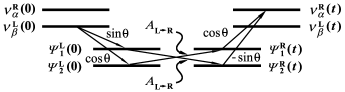
Figure 1: The schematic illustration of the system evolution in the case $\mu\gg\mu_{1,2}$. The horizontal lines of the figure correspond to various neutrino eigenstates at different moments of time ($t=0$ and $t$). The expressions next to arrows correspond to the appropriate factors in the formula (IV) of the wave function. The arrows from $\nu_{\beta}^{\mathrm{L}}(0)$ to $\psi_{1}^{\mathrm{L}}(0)$ and $\psi_{2}^{\mathrm{L}}(0)$, for example, indicate the vacuum mixing matrix transformation at $t=0$ and the arrow from $\psi_{1}^{\mathrm{L}}(0)$ to $\psi_{2}^{\mathrm{R}}(t)$ the evolution of the mass eigenstates with the helicity change. The transitions $\psi_{a}^{\mathrm{L}}(0)\to\psi_{b}^{\mathrm{R}}(t)$ can be described by the formula, $\psi_{1,2}^{\mathrm{R}}(t)=A_{\mathrm{L}\to\mathrm{R}}\psi_{2,1}^{\mathrm{L}}(0)$, where $A_{\mathrm{L}\to\mathrm{R}}=\mathrm{i}(\mu B/\Omega)\sin\Omega t$. This figure is taken from Ref. DvoMaa07 .

It should be noticed that the analog of Eq. (64) was obtained in Ref. LimMar88 where the authors studied the resonant spin flavor precession of Dirac and Majorana neutrinos in matter under the influence of an external magnetic field in frames of the quantum mechanical approach.

Using Eq. (IV) one can describe spin flavor oscillations of Dirac neutrinos with arbitrary magnetic moments matrix. It is the new result which was obtained using the relativistic quantum mechanics approach. Nevertheless this result is consistent with the conventional quantum mechanical description of spin flavor oscillations. We will demonstrate the consistency in Sec. V where more general case of neutrinos propagating in matter and external magnetic field is studied.

Spin flavor oscillations of Dirac neutrinos with arbitrary initial condition, not necessarily corresponding to ultrarelativistic particles, were studied in Ref. DvoMaa07 using the perturbative approach. To effectively apply the perturbation theory one has to study the situation of small transition magnetic moment, $\mu\ll\mu_{a}$. One could derive Eq. (IV) using the results of Ref. DvoMaa07 in the limit $k\gg m_{a}$.

V Dirac neutrinos in matter under the influence of a magnetic field

In this section, using the relativistic quantum mechanics method, we study the general case of the mixed flavor neutrinos propagating in background matter and interacting with an external electromagnetic field Dvo10 . We formulate the initial condition problem for neutrino spin flavor oscillations. Then we derive the effective Hamiltonian which governs spin flavor oscillations and show the consistence of our approach to the usual quantum mechanics method. The corrections to the standard effective Hamiltonian are also obtained.

The Lagrangian for the system of two mixed flavor neutrinos $\nu=(\nu_{\alpha},\nu_{\beta})$ interacting with background matter and external electromagnetic field has the form,

$$\mathcal{L}= \sum_{\lambda=\alpha,\beta}\bar{\nu}_{\lambda}\mathrm{i}\gamma^{\mu}\partial_{\mu}\nu_{\lambda}-\sum_{\lambda\lambda^{\prime}=\alpha,\beta}\bar{\nu}_{\lambda}\Big{(}m_{\lambda\lambda^{\prime}}+\gamma_{\mu}^{\mathrm{L}}f^{\mu}_{\lambda\lambda^{\prime}}$$

$$+\frac{1}{2}M_{\lambda\lambda^{\prime}}\sigma_{\mu\nu}F^{\mu\nu}\Big{)}\nu_{\lambda^{\prime}},$$ (65)

where the mass matrix $(m_{\lambda\lambda^{\prime}})$, matter interaction matrix $(f^{\mu}_{\lambda\lambda^{\prime}})$, and the magnetic moments matrix $(M_{\lambda\lambda^{\prime}})$ are defined in Secs. II, III, and IV respectively.

In the following we will be interested in the standard model neutrino interaction with matter which corresponds to the diagonal matrix $f^{\mu}_{\lambda\lambda^{\prime}}=\delta_{\lambda\lambda^{\prime}}f^{\mu}_{\lambda}$. Moreover we will study the situation of nonmoving and unpolarized matter. In this case only zero-th component of the four vector $f^{\mu}_{\lambda}$ is not equal to zero. The explicit form of this component $f_{\lambda}\equiv f^{0}_{\lambda}$ for the background matter composed of electrons, protons, and neutrons is given in Eq. (III).

We choose the configuration of the electromagnetic field $F_{\mu\nu}=(\mathbf{E},\mathbf{B})$ in Eq. (V) in the same form as in Sec. IV. Namely, we suppose that the electric field is absent $\mathbf{E}=0$ and magnetic field is constant and directed along the $z$-axis, $\mathbf{B}=(0,0,B)$.

To study the time evolution of flavor neutrinos we should supply the Lagrangian (V) with some initial condition. We choose the initial wave functions in the same form as in Sec. IV, i.e. we suppose that $\nu_{\alpha}(\mathbf{r},0)=0$ and $\nu_{\beta}(\mathbf{r},0)=e^{\mathrm{i}kx}\nu_{\beta}^{(0)}$, where the spinor $\nu_{\beta}^{(0)}$ corresponds to either left or right polarized neutrinos. The explicit form of $\nu_{\beta}^{(0)}$ can be defined with help of the operators $P_{\pm{}}$ in Eq. (43). It means that initially we have a beam of neutrinos of the flavor “$\beta$” with a specific polarization propagating along the $x$-axis. If we study the appearance of neutrinos of the flavor “$\alpha$” of the opposite polarization, it will correspond to a typical situation of neutrino spin flavor oscillations in matter and transversal magnetic field, $\nu_{\beta}^{\mathrm{L,R}}\leftrightarrow\nu_{\alpha}^{\mathrm{R,L}}$.

Then we introduce the mass eigenstates $\psi_{a}$ using Eqs. (3) and (4) to diagonalize the mass matrix $(m_{\lambda\lambda^{\prime}})$ in Eq. (V). These mass eigenstates are again supposed to be Dirac particles. Now the Lagrangian (V) expressed via the new mass eigenstates has the form,

$$\mathcal{L}= \sum_{a=1,2}\bar{\psi}_{a}(\mathrm{i}\gamma^{\mu}\partial_{\mu}-m_{a})\psi_{a}$$

$$-\sum_{ab=1,2}\bar{\psi}_{a}\left(g_{ab}^{\mu}\gamma_{\mu}^{\mathrm{L}}+\frac{1}{2}\mu_{ab}\sigma_{\mu\nu}F^{\mu\nu}\right)\psi_{b},$$ (66)

where $(g_{ab}^{\mu})$ and $(\mu_{ab})$ are the matrix of neutrino interaction with matter and the neutrino magnetic moments matrix expressed in the mass eigenstates basis, which are defined in Eqs. (25) and (45). We remind that in case of nonmoving and unpolarized matter the matrix $(g_{ab}^{\mu})$ has only zero-th component (27).

On the basis of the mass eigenstates Lagrangian (V), we can derive the corresponding wave equations which have the following form:

$$\mathrm{i}\dot{\psi}_{a}= \mathcal{H}_{a}\psi_{a}+\mathcal{V}\psi_{b},\quad a=1,2,\quad a\neq b,$$

$$\mathcal{H}_{a}= (\bm{\alpha}\mathbf{p})+\beta m_{a}-\mu_{a}\beta\Sigma_{3}B+g_{a}(1-\gamma^{5})/2,$$

$$\mathcal{V}= -\mu\beta\Sigma_{3}B+g(1-\gamma^{5})/2.$$ (67)

Note that we cannot directly solve the wave equations (V) because of the nondiagonal interaction $\mathcal{V}$ which mixes different mass eigenstates (see also Secs. III and IV). Nevertheless we can point out an exact solution of the wave equation $\mathrm{i}\dot{\psi}_{a}=\mathcal{H}_{a}\psi_{a}$, for a single mass eigenstate $\psi_{a}$, that exactly accounts for the influence of the external fields $g_{a}$ and $\mu_{a}B$. The contribution of the mixing potential $\mathcal{V}$ can be then taken into account using the perturbation theory, with all the terms in the expansion series being accounted for exactly.

We look for the solution of Eq. (V) in the following form Dvo10 :

$$\psi_{a}(\mathbf{r},t)= e^{-\mathrm{i}g_{a}t/2}\int\frac{\mathrm{d}^{3}\mathbf{p}}{(2\pi)^{3/2}}e^{\mathrm{i}\mathbf{p}\mathbf{r}}$$

$$\times\sum_{\zeta=\pm 1}\Big{[}a_{a}^{(\zeta)}(t)u_{a}^{(\zeta)}\exp{(-\mathrm{i}E_{a}^{(\zeta)}t)}$$

$$+b_{a}^{(\zeta)}(t)v_{a}^{(\zeta)}\exp{(\mathrm{i}E_{a}^{(\zeta)}t)}\Big{]},$$ (68)

where the energy levels, which were found in Ref. Dvo08JPG , have the form,

$$E^{(\zeta)}_{a}= \sqrt{\mathcal{M}^{2}_{a}+m^{2}_{a}+p^{2}-2\zeta R^{2}_{a}},$$

$$\mathcal{M}_{a}= \sqrt{(\mu_{a}B)^{2}+g_{a}^{2}/4},$$ (69)

where $R^{2}_{a}=\sqrt{p^{2}\mathcal{M}^{2}_{a}+(\mu_{a}B)^{2}m^{2}_{a}}$.

The basis spinors in Eq. (V) can be found in the limit of the small neutrino mass Dvo08JPG ,

$$u^{(\zeta)}_{a}= \frac{1}{2\sqrt{2\mathcal{M}_{a}(\mathcal{M}_{a}-\zeta g_{a}/2)}}\begin{pmatrix}\mu_{a}B+\zeta\mathcal{M}_{a}-g_{a}/2\\ \mu_{a}B-\zeta\mathcal{M}_{a}+g_{a}/2\\ \mu_{a}B-\zeta\mathcal{M}_{a}+g_{a}/2\\ \mu_{a}B+\zeta\mathcal{M}_{a}-g_{a}/2\ \end{pmatrix},$$

$$v^{(\zeta)}_{a}= \frac{1}{2\sqrt{2\mathcal{M}_{a}(\mathcal{M}_{a}+\zeta g_{a}/2)}}\begin{pmatrix}\mathcal{M}_{a}-\zeta[\mu_{a}B-g_{a}/2]\\ \mathcal{M}_{a}+\zeta[\mu_{a}B+g_{a}/2]\\ -\mathcal{M}_{a}-\zeta[\mu_{a}B+g_{a}/2]\\ -\mathcal{M}_{a}+\zeta[\mu_{a}B-g_{a}/2]\ \end{pmatrix}.$$ (70)

It should be noted that the discrete quantum number $\zeta=\pm 1$ in Eqs. (V)-(V) does not correspond to the helicity quantum states.

Now our goal is to find the time dependent coefficients $a_{a}^{(\zeta)}(t)$ and $b_{a}^{(\zeta)}(t)$. On the basis of the general solution (V) of the wave equation (V) we obtain the ordinary differential equations for these functions which formally coincide with Eq. (III). However the mixing potential $\mathcal{V}$ is now defined in Eq. (V). To obtain the modified Eq. (III) we again use the orthonormality of the basis spinors (V). The initial condition for the functions $a_{a}^{(\zeta)}(t)$ and $b_{a}^{(\zeta)}(t)$ also coincide with Eq. (III), with $\nu_{\beta}^{(0)}$ corresponding to a definite helicity spinor.

Taking into account the fact that $\langle u^{(\zeta)}_{a}|\mathcal{V}|v^{(\zeta^{\prime})}_{b}\rangle=0$, we get that the equations for $a_{a}^{(\zeta)}(t)$ and $b_{a}^{(\zeta)}(t)$ decouple, i.e. the interaction $\mathcal{V}$ does not mix positive and negative energy eigenstates. In the following we will consider the evolution of only $a_{a}^{(\zeta)}(t)$ since the dynamics of $b_{a}^{(\zeta)}(t)$ is studied analogously.

Let us rewrite the modified Eq. (III) in the more conventional effective Hamiltonian form. For this purpose we introduce the “wave function” $\Psi^{{}^{\prime}\mathrm{T}}=(a_{1}^{-{}},a_{2}^{-{}},a_{1}^{+{}},a_{2}^{+{}})$. Directly from the modified Eq. (III) for the functions $a_{a}^{(\zeta)}(t)$ we derive the equation for $\Psi^{\prime}$,

$$\mathrm{i}\frac{\mathrm{d}\Psi^{\prime}}{\mathrm{d}t}=H^{\prime}\Psi^{\prime},\quad H^{\prime}=\begin{pmatrix}0&h_{-{}}e^{\mathrm{i}\omega_{-{}}t}&0&H_{-{}}e^{\mathrm{i}\Omega_{-{}}t}\\ h_{-{}}e^{-\mathrm{i}\omega_{-{}}t}&0&H_{+{}}e^{-\mathrm{i}\Omega_{+{}}t}&0\\ 0&H_{+{}}e^{\mathrm{i}\Omega_{+{}}t}&0&h_{+{}}e^{\mathrm{i}\omega_{+{}}t}\\ H_{-{}}e^{-\mathrm{i}\Omega_{-{}}t}&0&h_{+{}}e^{-\mathrm{i}\omega_{+{}}t}&0\ \end{pmatrix},$$ (71)

where

$$h_{\mp{}}= \langle u^{\mp{}}_{a}|\mathcal{V}|u^{\mp{}}_{b}\rangle=\frac{1}{8\sqrt{\mathcal{M}_{a}\mathcal{M}_{b}(\mathcal{M}_{a}\pm g_{a}/2)(\mathcal{M}_{b}\pm g_{b}/2)}}$$

$$\times[2\mu B(g_{a}\mu_{b}B+g_{b}\mu_{a}B)\pm 4\mu B(\mu_{a}B\mathcal{M}_{b}+\mu_{b}B\mathcal{M}_{a})\pm 2g(g_{a}\mathcal{M}_{b}+g_{b}\mathcal{M}_{a})+4g\mathcal{M}_{a}\mathcal{M}_{b}+gg_{a}g_{b}],\quad a\neq b,$$

$$H_{\mp{}}= \langle u^{\mp{}}_{1}|\mathcal{V}|u^{\pm{}}_{2}\rangle=\langle u^{\pm{}}_{2}|\mathcal{V}|u^{\mp{}}_{1}\rangle=\frac{1}{8\sqrt{\mathcal{M}_{1}\mathcal{M}_{2}(\mathcal{M}_{1}\pm g_{1}/2)(\mathcal{M}_{2}\mp g_{2}/2)}}$$

$$\times[2\mu B(g_{1}\mu_{2}B+g_{2}\mu_{1}B)\mp 4\mu B(\mu_{1}B\mathcal{M}_{2}-\mu_{2}B\mathcal{M}_{1})\mp 2g(g_{1}\mathcal{M}_{2}-g_{2}\mathcal{M}_{1})-4g\mathcal{M}_{1}\mathcal{M}_{2}+gg_{1}g_{2}],$$ (72)

as well as $\omega_{\mp{}}=E_{1}^{\mp{}}-E_{2}^{\mp{}}+(g_{1}-g_{2})/2$ and $\Omega_{\mp{}}=E_{1}^{\mp{}}-E_{2}^{\pm{}}+(g_{1}-g_{2})/2$.

Instead of $\Psi^{\prime}$ it is more convenient to use the transformed “wave function” $\Psi$ defined by

$$\Psi^{\prime}=\mathcal{U}\Psi,\quad\mathcal{U}=\mathrm{diag}\left\{e^{\mathrm{i}(\Omega+\omega_{-{}})t/2},e^{\mathrm{i}(\Omega-\omega_{-{}})t/2},e^{-\mathrm{i}(\Omega-\omega_{+{}})t/2},e^{-\mathrm{i}(\Omega+\omega_{+{}})t/2}\right\},$$ (73)

where $\Omega=(\Omega_{-{}}-\Omega_{+{}})/2$, to exclude the explicit time dependence of the effective Hamiltonian $H^{\prime}$. Using the property $\omega_{+{}}+\omega_{-{}}=\Omega_{+{}}+\Omega_{-{}}$, we arrive to the new Schrödinger equation for the “wave function” $\Psi$,

$$\mathrm{i}\frac{\mathrm{d}\Psi}{\mathrm{d}t}=H\Psi,\quad H=\mathcal{U}^{\dagger}H^{\prime}\mathcal{U}-\mathrm{i}\mathcal{U}^{\dagger}\dot{\mathcal{U}}=\begin{pmatrix}(\Omega+\omega_{-{}})/2&h_{-{}}&0&H_{-{}}\\ h_{-{}}&(\Omega-\omega_{-{}})/2&H_{+{}}&0\\ 0&H_{+{}}&-(\Omega-\omega_{+{}})/2&h_{+{}}\\ H_{-{}}&0&h_{+{}}&-(\Omega+\omega_{+{}})/2\ \end{pmatrix}.$$ (74)

Despite initially we used perturbation theory to account for the influence of the potential $\mathcal{V}$ on the dynamics of the system (V), the contribution of this potential is taken into account exactly in Eq. (74). It means that our method allows one to sum up all terms in the perturbation series.

As we mentioned above, the quantum number $\zeta$ does not correspond to a definite helicity eigenstate. Thus the initial condition, which we should add to Eq. (74), has to be derived from Eqs. (III) and (V) and also depend on the neutrino oscillations channel. For example, if we discuss $\nu_{\beta}^{\mathrm{L}}\to\nu_{\alpha}^{\mathrm{R}}$ neutrino oscillations, the proper initial condition for the “wave function” $\Psi(0)=\Psi_{0}$ is

$$\Psi_{0}^{\mathrm{T}}=\left(-\sin\theta\sqrt{\frac{\mathcal{M}_{1}+g_{1}/2}{2\mathcal{M}_{1}}},-\cos\theta\sqrt{\frac{\mathcal{M}_{2}+g_{2}/2}{2\mathcal{M}_{2}}},\sin\theta\sqrt{\frac{\mathcal{M}_{1}-g_{1}/2}{2\mathcal{M}_{1}}},\cos\theta\sqrt{\frac{\mathcal{M}_{2}-g_{2}/2}{2\mathcal{M}_{2}}}\right).$$ (75)

Suppose that one has found the solution of the system (74) and (75) as $\Psi^{\mathrm{T}}(t)=(\psi_{1},\psi_{2},\psi_{3},\psi_{4})$. Then the transition probability for $\nu_{\beta}^{\mathrm{L}}\to\nu_{\alpha}^{\mathrm{R}}$ oscillations channel can be found as

$$P_{\nu_{\beta}^{\mathrm{L}}\to\nu_{\alpha}^{\mathrm{R}}}(t)= \frac{1}{2}\Bigg{\{}\frac{\mu_{1}B\cos\theta}{\sqrt{\mathcal{M}_{1}}}\left[\frac{\psi_{1}(t)}{\sqrt{\mathcal{M}_{1}+g_{1}/2}}+\frac{\psi_{3}(t)}{\sqrt{\mathcal{M}_{1}-g_{1}/2}}\right]$$

$$-\frac{\mu_{2}B\sin\theta}{\sqrt{\mathcal{M}_{2}}}\left[\frac{\psi_{2}(t)}{\sqrt{\mathcal{M}_{2}+g_{2}/2}}+\frac{\psi_{4}(t)}{\sqrt{\mathcal{M}_{2}-g_{2}/2}}\right]\Bigg{\}}^{2}.$$ (76)

To obtain Eq. (V) for simplicity we use the fact that initially we have rather broad (in space) wave packet, corresponding to the initial condition $\nu_{\beta}(\mathbf{r},0)=e^{\mathrm{i}kx}\nu_{\beta}^{(0)\mathrm{L}}$ [see Eq. (18)].

Now we demonstrate the consistency of the results of relativistic quantum mechanics approach to the description of neutrino spin flavor oscillations (see Eqs. (74)-(V), which look completely new) with the standard quantum mechanical method developed in Ref. LimMar88 . We remind that the following effective Hamiltimian:

$$H_{QM}^{\prime}=\begin{pmatrix}\Phi+g_{1}&g&-\mu_{1}B&-\mu B\\ g&-\Phi+g_{2}&-\mu B&-\mu_{2}B\\ -\mu_{1}B&-\mu B&\Phi&0\\ -\mu B&-\mu_{2}B&0&-\Phi\ \end{pmatrix},$$ (77)

was proposed in Ref. LimMar88 to describe the evolution of neutrino mass eigenstates in matter under the influence of an external magnetic field.

The effective Hamiltonian $H_{QM}^{\prime}$ acts in the space with the basis composed of helicity eigenstates of massive neutrinos. As we mentioned above, the helicity operator $(\bm{\Sigma}\mathbf{p})/|\mathbf{p}|$ does not commute with the Hamiltonian $\mathcal{H}_{a}$ in Eq. (V). Therefore the choice of the helicity eigenstates as the basis functions is justified only in the relatively weak external magnetic field case (see the detailed discussion in Ref. Dvo10 ) or in case of the small diagonal magnetic moments DvoMaa09 . In our approach we use the basis spinors (V) which are the eigenfunctions of the Hamiltonian $\mathcal{H}_{a}$ and exactly take into account matter density and magnetic field strength. Thus these spinors are more appropriate basis functions for the description of spin flavor oscillations.

We have found that in frames of the relativistic quantum mechanics approach the dynamics of the neutrino system can be described by the Schrödinger like equation with the effective Hamiltonian (74). Let us decompose the energy levels (V) supposing that neutrinos are ultrarelativistic particles,

$$E_{a}^{(\zeta)}=k+\frac{g_{a}}{2}-\zeta\mathcal{M}_{a}+\frac{m_{a}^{2}}{2k}+\zeta\frac{m_{a}^{2}g_{a}^{2}}{8k^{2}\mathcal{M}_{a}}+\dotsb.$$ (78)

In Eq. (78) we keep the term $\sim m_{a}^{2}/k^{2}$ to examine the corrections to the conventional quantum mechanical approach.

Performing the similarity transformation of the effective Hamiltonian $H$ in Eq. (74) and using the orthogonal matrix $\mathcal{R}$ ($\mathcal{R}^{\mathrm{T}}\mathcal{R}=I$) of the following form:

$$\mathcal{R}=\begin{pmatrix}\displaystyle-\frac{\sqrt{\mathcal{M}_{1}+g_{1}/2}}{\sqrt{2\mathcal{M}_{1}}}&0&\displaystyle\frac{\mu_{1}B}{\sqrt{2\mathcal{M}_{1}(\mathcal{M}_{1}+g_{1}/2)}}&0\\ 0&\displaystyle-\frac{\sqrt{\mathcal{M}_{2}+g_{2}/2}}{\sqrt{2\mathcal{M}_{2}}}&0&\displaystyle\frac{\mu_{2}B}{\sqrt{2\mathcal{M}_{2}(\mathcal{M}_{2}+g_{2}/2)}}\\ \displaystyle\frac{\sqrt{\mathcal{M}_{1}-g_{1}/2}}{\sqrt{2\mathcal{M}_{1}}}&0&\displaystyle\frac{\mu_{1}B}{\sqrt{2\mathcal{M}_{1}(\mathcal{M}_{1}-g_{1}/2)}}&0\\ 0&\displaystyle\frac{\sqrt{\mathcal{M}_{2}-g_{2}/2}}{\sqrt{2\mathcal{M}_{2}}}&0&\displaystyle\frac{\mu_{2}B}{\sqrt{2\mathcal{M}_{2}(\mathcal{M}_{2}-g_{2}/2)}}\ \end{pmatrix},$$ (79)

we can see that the Hamiltonian $H$ transforms to $\mathcal{R}^{\mathrm{T}}H\mathcal{R}\approx H_{QM}+\delta H$, where

$$H_{QM}=\\ \begin{pmatrix}\Phi+3g_{1}/4-g_{2}/4&g&-\mu_{1}B&-\mu B\\ g&-\Phi+3g_{2}/4-g_{1}/4&-\mu B&-\mu_{2}B\\ -\mu_{1}B&-\mu B&\Phi-(g_{1}+g_{2})/4&0\\ -\mu B&-\mu_{2}B&0&-\Phi-(g_{1}+g_{2})/4\ \end{pmatrix},$$ (80)

and

$$\delta H=\frac{1}{16k^{2}}\mathrm{diag}\left(-m_{1}^{2}\frac{g_{1}^{3}}{\mathcal{M}_{1}^{2}},-m_{2}^{2}\frac{g_{2}^{3}}{\mathcal{M}_{2}^{2}},m_{1}^{2}\frac{g_{1}^{3}}{\mathcal{M}_{1}^{2}},m_{2}^{2}\frac{g_{2}^{3}}{\mathcal{M}_{2}^{2}}\right),$$ (81)

is the correction to the standard effective Hamiltonian. It should be noted that the transformation matrix $\mathcal{R}$ in Eq. (79) depends on the magnetic field strength and the matter density.

The effective Hamiltonian $H_{QM}$ is equivalent to $H^{\prime}_{QM}$ in Eq. (77) since $H_{QM}=H^{\prime}_{QM}-\mathrm{tr}(H^{\prime}_{QM})/4\cdot I$, where $I$ is the $4\times 4$ unit matrix. It is known that the unit matrix does not change the particles dynamics. Thus the relativistic quantum mechanics approach is equivalent to the standard approach developed in Ref. LimMar88 .

Now let us discuss the correction $\delta H$ [see Eq. (81)] to the quantum mechanical method. This correction results from the fact that we use the correct energy levels for a neutrino moving in dense matter and strong magnetic field. Note that in Eq. (81) we keep only the diagonal corrections $\sim m_{a}^{2}/k^{2}$ to the effective Hamiltonian (80). If we slightly change non-diagonal elements of the Hamiltonian, it will result in the small changes of the transition probability. However, if we add some small quantity to diagonal elements, it can produce the resonance enhancement of neutrino oscillations.

We should remind that the expressions for the basis spinors (V) were obtained in the approximation of neutrinos with small masses, whereas in Eq. (78) we expand the energy up to $\sim m_{a}^{2}/k^{2}$ terms. If we take into account $\sim m_{a}^{2}/k^{2}$ corrections to the basis spinors (V), we can expect that some non-diagonal entries in the effective Hamiltonian $H$ (74) will also obtain $\sim m_{a}^{2}/k^{2}$ corrections: $h_{\pm{}}\to h_{\pm{}}+\delta h_{\pm{}}$ and $H_{\pm{}}\to H_{\pm{}}+\delta H_{\pm{}}$. However, using the explicit form of the effective Hamiltonian $H$ (74) and the matrix $\mathcal{R}$ (79) we get that these additional contributions are washed out in diagonal entries in Eq. (81). We analyze the validity of the approximations made in the derivation of the correction (81) in Appendix B.

VI Spin flavor oscillations of Dirac neutrinos in the magnetized envelope of a supernova

In this section we study the application of the general formalism for the description of neutrino spin flavor oscillations, developed in Sec. V, to the situation of neutrinos propagating in the expanding envelope formed after a supernova explosion DvoMaa09 . We find an exact solution of the Schrödinger equation with the effective Hamiltonian (80) for the background matter profile present in an expanding envelope and in the supernova magnetic field. We also analyze the possibility of enhancement of neutrino oscillations.

To describe the dynamics of neutrino spin flavor oscillations one has to solve the evolution equation with the Hamiltonian (80). This problem, in its turn, requires to solve a secular equation which is the fourth-order algebraic equation in order to find the eigenvalues of the effective Hamiltonian. Although one can express the solution to such an equation in radicals, its actual form appears to be rather cumbersome for arbitrary parameters.

If we, however, consider the case of a neutrino propagating in the electrically neutral isoscalar matter, i.e. $n_{e}=n_{p}$ and $n_{p}=n_{n}$, a reasonable solution is possible to find. We will demonstrate later that it corresponds to a realistic physical situation. As one can infer from Eq. (III) for the case of the $\nu_{e}^{\mathrm{L}}\to\nu_{\mu}^{\mathrm{R}}$ oscillations channel, in a medium with this property one has the effective potentials $f_{\alpha}\equiv f_{\mu}=V_{\mu}=-G_{\mathrm{F}}n/\sqrt{2}$ and $f_{\beta}\equiv f_{e}=V_{e}=G_{\mathrm{F}}n/\sqrt{2}$, where $n\equiv n_{e}=n_{p}=n_{n}$. Using Eq. (37) we obtain that $g_{1}=-g_{2}=g_{0}$, where $g_{0}=-V\cos 2\theta$, $g=V\sin 2\theta$, and $V=G_{\mathrm{F}}n/\sqrt{2}$.

Let us point out that background matter with these properties may well exist in some astrophysical environments. The matter profile of presupernovae is poorly known, and a variety of presupernova models with different profiles exist in the literature (see, e.g., Ref. WooHegWea02 ). Nevertheless, electrically neutral isoscalar matter may well exist in the inner parts of presupernovae consisting of elements heavier than hydrogen. Indeed, for example, the model W02Z in Ref. WooHegWea02 predicts that in a 15$M_{\odot}$ presupernova one has $Y_{e}=n_{e}/(n_{p}+n_{n})=0.5$ in the O+Ne+Mg layer, between the Si+O and He layers, in the radius range (0.007–0.2)$R_{\odot}$.

We also discuss the model of neutrino magnetic moments in which the nondiagonal elements of the magnetic moments matrix (45) are much bigger than the diagonal magnetic moments. Such a magnetic moments matrix was previously discussed in our works DvoMaa07 ; Dvo08JPG ; DvoMaa09 (see also Sec. IV). Note that in case of negligible diagonal magnetic moments the helicity operator (43) commutes with the Hamiltonian $\mathcal{H}_{a}$ in Eq. (V) and hence the effective Hamiltonian (80) acts in the helicity eigenstates basis. In other words the effective Hamiltonian (77) proposed in the standard quantum mechanical approach LimMar88 is justified in our case.

For neutrinos having such magnetic moments and propagating in isoscalar matter the effective Hamiltonian (80) is replaced by

$$H_{QM}\to\begin{pmatrix}\Phi+g_{0}&g&0&-\mu B\\ g&-(\Phi+g_{0})&-\mu B&0\\ 0&-\mu B&\Phi&0\\ -\mu B&0&0&-\Phi\ \end{pmatrix}.$$ (82)

We now look for the stationary solutions of the Schrödinger equation with this Hamiltonian. After a straightforward calculation one finds

$$\Psi(t)= \sum_{\zeta=\pm 1}\Big{[}\left(U_{\zeta}\otimes U_{\zeta}^{\dagger}\right)\exp{(-\mathrm{i}\mathcal{E}_{\zeta}t)}$$

$$+\left(V_{\zeta}\otimes V_{\zeta}^{\dagger}\right)\exp{(\mathrm{i}\mathcal{E}_{\zeta}t)}\Big{]}\Psi_{0},$$ (83)

where we have denoted

$$\mathcal{E}_{\pm{}}= \frac{1}{2}\sqrt{2V^{2}+4(\mu B)^{2}+4\Phi^{2}-4\Phi V\cos 2\theta\pm 2VR},$$

$$R= \sqrt{(V-2\Phi\cos 2\theta)^{2}+4(\mu B)^{2}}.$$ (84)

The vectors $U_{\pm{}}$ and $V_{\pm{}}$ are the eigenvectors corresponding to the energy eigenvalues $\mathcal{E}_{\pm{}}$ and $-\mathcal{E}_{\pm{}}$, respectively. They are given by ($\zeta=\pm{}$)

$$U_{\zeta}= \frac{1}{N_{\zeta}}\begin{pmatrix}Z_{\zeta}\\ \sin 2\theta(\mathcal{E}_{\zeta}-\Phi)\\ -\mu B\sin 2\theta\\ -\mu BZ_{\zeta}/(\mathcal{E}_{\zeta}+\Phi)\ \end{pmatrix},$$

$$V_{\zeta}= \frac{1}{N_{\zeta}}\begin{pmatrix}-\sin 2\theta(\mathcal{E}_{\zeta}-\Phi)\\ Z_{\zeta}\\ \mu BZ_{\zeta}/(\mathcal{E}_{\zeta}+\Phi)\\ -\mu B\sin 2\theta\ \end{pmatrix},$$ (85)

where

$$Z_{\zeta}= \frac{V+\zeta R}{2}-\mathcal{E}_{\zeta}\cos 2\theta,$$

$$N_{\zeta}^{2}= Z_{\zeta}^{2}\left[1+\frac{(\mu B)^{2}}{(\mathcal{E}_{\zeta}+\Phi)^{2}}\right]$$

$$+\sin^{2}(2\theta)\left[(\mu B)^{2}+(\mathcal{E}_{\zeta}-\Phi)^{2}\right].$$ (86)

It should be noted that Eq. (VI) is a general solution of the evolution equation with the effective Hamiltonian (82) satisfying the initial condition $\Psi(0)=\Psi_{0}$.

Note that we received the solution (VI)-(VI) under some assumptions on the external fields such as isoscalar matter with constant density and constant magnetic field. In Sec. V we showed that our method is equivalent to the quantum mechanical description of neutrino oscillations LimMar88 which can be used for a more general case of coordinate dependent external fields. Nevertheless the assumption of constant matter density and magnetic field is quite realistic for certain astrophysical environments like a shock wave propagating inside an expanding envelope after a supernova explosion.

Consistently with Eqs. (2)-(4), and (18) with an initial spinor $\nu_{\beta}^{(0)}$ corresponding to a left polarized neutrino (43), we take the initial wave function $\Psi(0)\equiv\Psi_{0}$ in Eq. (VI) as $\Psi_{0}^{\mathrm{T}}=(\psi_{1}^{\mathrm{L}},\psi_{2}^{\mathrm{L}},\psi_{1}^{\mathrm{R}},\psi_{2}^{\mathrm{R}})=(\sin\theta,\cos\theta,0,0)$. Using Eqs. (VI)-(VI) one finds the components of the quantum mechanical wave function corresponding to the right polarized neutrinos to be of the form

$$\psi_{1}^{\mathrm{R}}(t)= \frac{\mu B}{N_{+{}}^{2}}\bigg{\{}\cos\theta\bigg{[}e^{\mathrm{i}\mathcal{E}_{+{}}t}\frac{Z_{+{}}^{2}}{\mathcal{E}_{+{}}+\Phi}$$

$$-\sin^{2}(2\theta)(\mathcal{E}_{+{}}-\Phi)e^{-\mathrm{i}\mathcal{E}_{+{}}t}\bigg{]}$$

$$-\sin\theta\sin 2\theta Z_{+{}}\bigg{[}e^{-\mathrm{i}\mathcal{E}_{+{}}t}$$

$$+e^{\mathrm{i}\mathcal{E}_{+{}}t}\frac{\mathcal{E}_{+{}}-\Phi}{\mathcal{E}_{+{}}+\Phi}\bigg{]}\bigg{\}}+\{+{}\to{}-{}\},$$

$$\psi_{2}^{\mathrm{R}}(t)= \frac{\mu B}{N_{+{}}^{2}}\bigg{\{}\sin\theta\bigg{[}\sin^{2}(2\theta)(\mathcal{E}_{+{}}-\Phi)e^{\mathrm{i}\mathcal{E}_{+{}}t}$$

$$-e^{-\mathrm{i}\mathcal{E}_{+{}}t}\frac{Z_{+{}}^{2}}{\mathcal{E}_{+{}}+\Phi}\bigg{]}$$

$$-\cos\theta\sin 2\theta Z_{+{}}\bigg{[}e^{\mathrm{i}\mathcal{E}_{+{}}t}$$

$$+e^{-\mathrm{i}\mathcal{E}_{+{}}t}\frac{\mathcal{E}_{+{}}-\Phi}{\mathcal{E}_{+{}}+\Phi}\bigg{]}\bigg{\}}+\{+{}\to{}-{}\},$$ (87)

where the $\{+{}\to{}-{}\}$ stand for the terms similar to the terms preceding each of them but with all quantities with a subscript $+{}$ replaced with corresponding quantities with a subscript $-{}$. The wave function of the right-handed neutrino of the flavor “$\alpha$”, $\nu_{\alpha}^{\mathrm{R}}$, can be written with help of Eqs. (2)-(4), and (VI) as $\nu_{\alpha}^{\mathrm{R}}(t)=\cos\theta\psi_{1}^{\mathrm{R}}(t)-\sin\theta\psi_{2}^{\mathrm{R}}(t)$.

The probability for the transition $\nu_{\beta}^{\mathrm{L}}\to\nu_{\alpha}^{\mathrm{R}}$ is obtained as the square of the quantum mechanical wave function $\nu_{\alpha}^{\mathrm{R}}$. One obtains

$$P_{\nu_{\beta}^{\mathrm{L}}\to\nu_{\alpha}^{\mathrm{R}}}(t)= \left|\nu_{\alpha}^{\mathrm{R}}\right|^{2}$$

$$=[C_{+{}}\cos(\mathcal{E}_{+{}}t)+C_{-{}}\cos(\mathcal{E}_{-{}}t)]^{2}$$

$$+[S_{+{}}\sin(\mathcal{E}_{+{}}t)+S_{-{}}\sin(\mathcal{E}_{-{}}t)]^{2},$$ (88)

where ($\zeta=\pm$)

$$C_{\zeta}= \frac{\mu B}{N_{\zeta}^{2}}\left\{\frac{Z_{\zeta}^{2}}{\mathcal{E}_{\zeta}+\Phi}-\sin^{2}(2\theta)(\mathcal{E}_{\zeta}-\Phi)\right\},$$

$$S_{\zeta}= \frac{\mu B}{N_{\zeta}^{2}}\bigg{\{}\sin^{2}(2\theta)\frac{2\Phi Z_{\zeta}}{\mathcal{E}_{\zeta}+\Phi}$$

$$+\cos 2\theta\left[\frac{Z_{\zeta}^{2}}{\mathcal{E}_{\zeta}+\Phi}+\sin^{2}(2\theta)(\mathcal{E}_{\zeta}-\Phi)\right]\bigg{\}}.$$ (89)

As a consistency check, one easily finds from Eq. (VI) that $C_{+{}}+C_{-{}}=0$ as required for assuring $P(0)=0$.

In the following we will limit our considerations to the case $\mathcal{E}_{+{}}\approx\mathcal{E}_{-{}}$, corresponding to the situations where the effect of the interactions of neutrinos with matter ($V$) is small compared with that of the magnetic interactions ($\mu B$) or the vacuum contribution ($\Phi$) or both [see Eq. (VI)]. Note that in this case one can analyze the exact oscillation probability (VI) analytically, which would be practically impossible in more general situations.

In the case $\mathcal{E}_{+{}}\approx\mathcal{E}_{-{}}$, one can present the transition probability in Eq. (VI) in the following form:

$$P(t)=P_{0}(t)+P_{c}(t)\cos(2\Omega t)+P_{s}(t)\sin(2\Omega t),$$ (90)

where

$$P_{0}(t)= \frac{1}{2}\big{[}S_{+{}}^{2}+S_{-{}}^{2}+2S_{+{}}S_{-{}}\cos(2\delta\Omega t)$$

$$-4C_{+{}}C_{-{}}\sin^{2}(\delta\Omega t)\big{]},$$

$$P_{c}(t)= -\frac{1}{2}\big{[}(S_{+{}}^{2}+S_{-{}}^{2})\cos(2\delta\Omega t)+2S_{+{}}S_{-{}}$$

$$-4C_{+{}}C_{-{}}\sin^{2}(\delta\Omega t)\big{]},$$

$$P_{s}(t)= \frac{1}{2}\left(S_{+{}}^{2}-S_{-{}}^{2}\right)\sin(2\delta\Omega t),$$ (91)

and

$$\Omega=\frac{\mathcal{E}_{+{}}+\mathcal{E}_{-{}}}{2},\quad\delta\Omega=\frac{\mathcal{E}_{+{}}-\mathcal{E}_{-{}}}{2}.$$ (92)

As one can infer from these expressions, the transition probability $P(t)$ is a rapidly oscillating function, with the frequency $\Omega$, enveloped from up and down by the slowly varying functions $P_{u,d}=P_{0}\pm\sqrt{P_{c}^{2}+P_{s}^{2}}$, respectively.

The behavior of the transition probability for various matter densities $\rho$ and the values of $\mu B$ and for a fixed neutrino energy of $E=10\thinspace\text{MeV}$ and squared mass difference of $\delta m^{2}=8\times 10^{-5}\thinspace\text{eV}^{2}$ is illustrated in Figs. 2-4.

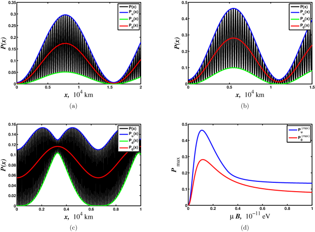
Figure 2: (color online) (a)-(c) The transition probability versus the distance passed by a neutrino beam in matter with the density $\rho=10\thinspace\text{g/cc}$; (a) $\mu B=5\times 10^{-13}\thinspace\text{eV}$, (b) $\mu B=1.1\times 10^{-12}\thinspace\text{eV}$, (c) $\mu B=5\times 10^{-12}\thinspace\text{eV}$. We take that $E_{\nu}=10\thinspace\text{MeV}$, $\delta m^{2}=8\times 10^{-5}\thinspace\text{eV}^{2}$ and $\theta=0.6$, which is quite close to the solar neutrinos’ oscillations parameters. The black line is the function $P(x)$, the blue and green lines are the envelope functions $P_{u,d}(x)$, and the red line is the averaged transition probability $P_{0}(x)$. (d) The dependence of the maximal values of the functions $P(x)$ and $P_{0}(x)$, blue and red lines, respectively, on the magnetic energy $\mu B$ for the given density. This figure is taken from Ref. DvoMaa09 .

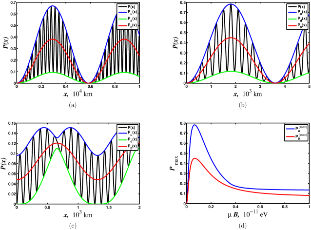
Figure 3: (color online) The same as in Fig. 2 for the density $\rho=50\thinspace\text{g/cc}$; (a) $\mu B=3.5\times 10^{-13}\thinspace\text{eV}$, (b) $\mu B=6.6\times 10^{-13}\thinspace\text{eV}$, (c) $\mu B=5\times 10^{-12}\thinspace\text{eV}$. After Ref. DvoMaa09 .

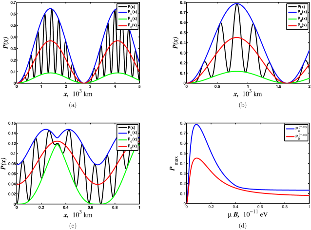
Figure 4: (color online) The same as in Fig. 2 for the density $\rho=100\thinspace\text{g/cc}$; (a) $\mu B=4\times 10^{-13}\thinspace\text{eV}$, (b) $\mu B=8\times 10^{-13}\thinspace\text{eV}$, (c) $\mu B=5\times 10^{-12}\thinspace\text{eV}$. After Ref. DvoMaa09 .

As these plots show, at low matter densities the envelope functions give, at each propagation distance, the range of the possible values of the oscillation probability. At greater matter densities, where the probability oscillates less intensively, the envelope functions are not that useful in analyzing the physical situation.

One can find the maximum value of the upper envelope function, which is also the upper bound for the transition probability, given as

$$P_{u}^{\mathrm{(max)}}=\begin{cases}(S_{+{}}-S_{-{}})^{2},&\text{if $B<B^{\prime}$},\\ \displaystyle\frac{C_{+{}}C_{-{}}(S_{+{}}^{2}-S_{-{}}^{2})^{2}}{C_{+{}}C_{-{}}(S_{+{}}^{2}+S_{-{}}^{2})+(C_{+{}}C_{-{}})^{2}+(S_{+{}}S_{-{}})^{2}},&\text{if $B>B^{\prime}$},\end{cases}$$ (93)

where the value $B^{\prime}$ is the solution of the transcendent algebraic equation, $C_{+{}}C_{-{}}=S_{+{}}S_{-{}}$. The corresponding maximum values of the averaged transition probability $P_{0}(x)$ are given by

$$P_{0}^{\mathrm{(max)}}=\frac{1}{2}[(S_{+{}}S_{-{}})^{2}-4C_{+{}}C_{-{}}],$$ (94)

for arbitrary values of $B$. The values of these maxima depend on the size of the quantity $\mu B$. These dependencies are plotted in Figs. 2(d)-4(d). In the case of rapid oscillations the physically relevant quantities, rather than the maxima, are the averaged values of the transition probability, which are also plotted in these figures.

As Figs. 2(d)-4(d) show, the interplay of the matter effect and the magnetic interaction can lead, for a given magnetic moment $\mu$, to an enhanced spin flavor transition if the magnetic field $B$ has a suitable strength relative to the density of matter $\rho$. In our numerical examples this occurs at $\mu B_{\mathrm{max}}=1.1\times 10^{-12}\thinspace\text{eV}$ for $\rho=10\thinspace\text{g/cc}$, at $\mu B_{\mathrm{max}}=6.6\times 10^{-13}\thinspace\text{eV}$ for $\rho=50\thinspace\text{g/cc}$, and at $\mu B_{\mathrm{max}}=8\times 10^{-13}\thinspace\text{eV}$ for $\rho=100\thinspace\text{g/cc}$. For these values of $\mu B$ both the maxima and the average of the transition probability become considerably larger than for any other values of $\mu B$. Figs. 2(b)-4(b) correspond to the situation of maximal enhancement, whereas Figs. 2(a)-4(a) and Figs. 2(c)-4(c) illustrate the situation above and below the optimal strength $B_{\mathrm{max}}$ of the magnetic field.

It is noteworthy that the enhanced transition probability is achieved towards the lower end of the $\mu B$ region where substantial transitions all occur, that is, at relatively moderate magnetic fields. At larger values of $\mu B$ the maximum of the transition probability approaches towards $\cos^{2}(2\theta)$. Indeed, if $\mu B\gg\max(\Phi,V)$, the transition probability can be written in the form $P(t)=\cos^{2}(2\theta)\sin^{2}(\mu Bt)$ [see Eq. (64)]. It was found in Ref. LikStu95 that neutrino spin flavor oscillations can be enhanced in a very strong magnetic field, with the transition probability being practically equal to unity. This phenomenon can be realized only for Dirac neutrinos with small nondiagonal magnetic moments and small mixing angle. As we can see from Figs. 2(d)-4(d) the situation is completely different for big nondiagonal magnetic moments.

One should notice that for long propagation distances consisting of several oscillation periods of the envelope functions, the enhancement effect would diminish considerably because of averaging. In the numerical examples presented in Figs. 2-4 the period of the envelope function is of the order of $10^{3}-10^{4}\thinspace\text{km}$, which is a typical size of a shock wave with the matter densities we have used in the plots (see, e.g., Ref. Kaw06 ). Thus the enhanced spin flavor transition could take place when neutrinos traverse a shock wave.

Let us recall that the above analysis was made by assuming neutrinos to be Dirac particles. We will see below (see Sec. X) that the corresponding results are quite different in the case of Majorana neutrinos.

VII Spin flavor oscillations between electron and sterile astrophysical neutrinos

In this section we continue with the studies of oscillations of supernova neutrinos on the basis of the effective Hamiltonian derived in Sec. V. In particular, we discuss the possibility of spin flavor oscillations between right polarized electron neutrino and additional sterile neutrino in an expanding envelope formed after a supernova explosion under the influence of a strong magnetic field. It is shown that the resonance enhancement of neutrino oscillations is possible if we take into account the correction to the effective Hamiltonian (81).

As we mentioned in Sec. VI, in general case the solution of the Schrödinger equation based on the effective Hamiltonians (80) and (81) is quite cumbersome and should be analyzed numerically. To study spin flavor oscillations analytically we consider, just for simplicity, the situation when the vacuum mixing angle between different neutrino eigenstates is small, $\theta\ll 1$. If $\theta\ll 1$, the matter interaction term and the the magnetic moments coincide in both flavor and mass eigenstates bases.

A resonance of neutrino oscillations can appear if the difference between two diagonal elements in the effective Hamiltonian is small AkhLanSci97 . In table 1, where we take into account the contributions of both Eqs. (80) and (81),

Table 1: The resonance conditions for the $\nu_{\alpha}^{\mathrm{L,R}}\leftrightarrow\nu_{\beta}^{\mathrm{L,R}}$ oscillations channels which take into account the Hamiltonians (80) and (81).

No.	Oscillations channel	Resonance condition
1	$\nu_{\beta}^{\mathrm{L}}\leftrightarrow\nu_{\alpha}^{\mathrm{R}}$	$\displaystyle\Phi=\frac{f_{\beta}}{2}-\frac{1}{32k^{2}}\left(\frac{m_{1}^{2}f_{\alpha}^{3}}{\mathcal{M}_{1}^{2}}+\frac{m_{2}^{2}f_{\beta}^{3}}{\mathcal{M}_{2}^{2}}\right)$
2	$\nu_{\beta}^{\mathrm{R}}\leftrightarrow\nu_{\alpha}^{\mathrm{L}}$	$\displaystyle\Phi=-\frac{f_{\alpha}}{2}+\frac{1}{32k^{2}}\left(\frac{m_{1}^{2}f_{\alpha}^{3}}{\mathcal{M}_{1}^{2}}+\frac{m_{2}^{2}f_{\beta}^{3}}{\mathcal{M}_{2}^{2}}\right)$
3	$\nu_{\beta}^{\mathrm{L}}\leftrightarrow\nu_{\alpha}^{\mathrm{L}}$	$\displaystyle\Phi=\frac{f_{\beta}-f_{\alpha}}{2}+\frac{1}{32k^{2}}\left(\frac{m_{1}^{2}f_{\alpha}^{3}}{\mathcal{M}_{1}^{2}}-\frac{m_{2}^{2}f_{\beta}^{3}}{\mathcal{M}_{2}^{2}}\right)$
4	$\nu_{\beta}^{\mathrm{R}}\leftrightarrow\nu_{\alpha}^{\mathrm{R}}$	$\displaystyle\Phi=-\frac{1}{32k^{2}}\left(\frac{m_{1}^{2}f_{\alpha}^{3}}{\mathcal{M}_{1}^{2}}-\frac{m_{2}^{2}f_{\beta}^{3}}{\mathcal{M}_{2}^{2}}\right)$

we list the resonance conditions for various oscillations channels. It can be seen from this table that the corrections (81) to the effective Hamiltonian become important when we discuss $\nu_{e,\mu,\tau}^{\mathrm{R}}\leftrightarrow\nu_{s}^{\mathrm{L,R}}$ oscillations channel, where $\nu_{s}$ is the additional sterile neutrino.

As an example, we can study the case of $\nu_{e}^{\mathrm{R}}\leftrightarrow\nu_{s}^{\mathrm{L}}$ oscillations. Putting $\alpha\equiv s$ and $\beta\equiv e$ in table 1 and using Eq. (III), we obtain that $f_{s}=0$, $f_{e}=\sqrt{2}G_{\mathrm{F}}(n_{e}-n_{n}/2)$ and $\mathcal{M}_{2}\equiv\mathcal{M}_{e}=\sqrt{(\mu_{\nu_{e}}B)^{2}+f_{e}^{2}}$. From table 1 we obtain the resonance condition for this oscillations channel as,

$$\delta m^{2}=\frac{1}{4\sqrt{2}E_{\nu}}G_{\mathrm{F}}\left(n_{e}-\frac{n_{n}}{2}\right)m_{\nu_{e}}^{2},$$ (95)

where we discuss the case of small diagonal magnetic moment of an electron neutrino: $\mu_{\nu_{e}}B\ll f_{e}$ and $E_{\nu}=k$ is the neutrino energy. In Appendix B we discuss other small factors which can also contribute to the resonance condition (95).

As an example we consider $\nu_{e}^{\mathrm{R}}\leftrightarrow\nu_{s}^{\mathrm{L}}$ oscillations in an expanding envelope of a supernova explosion. It is known (see, e.g., Refs. Not88 ; BarMoh88 for the most detailed analysis) that right polarized electron neutrinos can be created during the explosion of a core-collapse supernova. Indeed, if a neutrino is a Dirac particle, the spin flip can occur in the following reaction: $\nu_{\mathrm{L}}+(e^{-{}},p,N)\to\nu_{\mathrm{R}}+(e^{-{}},p,N)$, with electrons $e^{-{}}$, protons $p$, and nuclei $N$ in the dense matter of a forming neutron star. This spin flip is due to the interaction of the neutrino diagonal magnetic moment with charged particles. Hence left polarized neutrinos are converted into right polarized ones with energy in the range $(100-200)\thinspace\text{MeV}$ AyaDOlTor00 .

Besides the fact that the creation of right polarized neutrinos can provide additional supernova cooling KuzMikOkr09 , these particles can be observed in a terrestrial detector. When right polarized neutrinos propagate from the supernova explosion site towards the Earth, interacting with the galactic magnetic field, their helicity can change back and they become left polarized neutrinos. Although the flux of this kind of neutrinos is smaller than that of generic left polarized neutrinos BarMoh88 ; LycBli10 , potentially we can detect these particles. The analysis of the neutrino spin precession in the galactic magnetic field is given in Ref. LycBli10 .

Suppose that the flux of right polarized electron neutrinos is crossing an expanding envelope of a supernova. A shock wave can be formed in the envelope Tom05 . Approximately $1\thinspace\text{s}$ after the core collapse, the matter density in the shock wave region $L\sim 10^{8}\thinspace\text{cm}$ can be up to $10^{6}\thinspace\text{g/cm}^{3}$. We can also suppose that the matter density is approximately constant inside the shock wave (see also Sec. VI).

For the electroneutral matter Eq. (95) reads

$$\delta m^{2}\approx 5.0\times 10^{-17}\thinspace\text{eV}^{2}\times(3Y_{e}-1)$$

$$\times\left(\frac{\rho}{10^{6}\thinspace\text{g/cm}^{3}}\right)\left(\frac{E_{\nu}}{100\thinspace\text{MeV}}\right)^{-1}\left(\frac{m_{\nu_{e}}}{1\thinspace\text{eV}}\right)^{2},$$ (96)

where $Y_{e}=n_{e}/(n_{e}+n_{n})$ is the electrons fraction. From Eq. (VII) we can see that for the matter with $Y_{e}>1/3$ and $\rho\sim 10^{6}\thinspace\text{g/cm}^{3}$ and an electron neutrino with $E_{\nu}\sim 100\thinspace\text{MeV}$ and $m_{\nu_{e}}\sim 1\thinspace\text{eV}$ the mass squared difference should be $\delta m^{2}\sim 10^{-17}\thinspace\text{eV}^{2}$.

Note that the possibility of existence of sterile neutrinos closely degenerate in mass with active neutrinos was recently discussed. In Ref. Ker03 it was examined how the fluxes of supernova neutrinos can be altered is presence of the almost degenerate neutrinos. The effect of spin flavor oscillations between active and sterile neutrinos with small $\delta m^{2}$ on the solar neutrino fluxes was discussed in Ref. snusolar . The implications of the CP phases of the mixing between active and sterile neutrinos in the scenario with small $\delta m^{2}$ to the effective mass of an electron neutrinos were considered in Ref. MaaRii10 . In Ref. Esm10 it was examined the possibility to experimentally confirm, e.g., in the IceCube detector, the existence of almost degenerate in masses sterile neutrinos emitted with high energies from extragalactic sources. The range of $\delta m^{2}$ studied in Ref. Ker03 is $10^{-16}\thinspace\text{eV}^{2}<\delta m^{2}<10^{-12}\thinspace\text{eV}^{2}$ which is quite close to the estimates obtained from Eq. (VII). In Ref. Esm10 the sterile neutrinos with even smaller $\delta m^{2}$ were studied: $10^{-19}\thinspace\text{eV}^{2}<\delta m^{2}<10^{-12}\thinspace\text{eV}^{2}$.

Besides the fulfillment of the resonance condition (95), to have the significant $\nu_{e}^{\mathrm{R}}\leftrightarrow\nu_{s}^{\mathrm{L}}$ transitions rate the strength of the magnetic field and distance traveled by the neutrinos beam, which we take to be equal to the shock wave size $L$, should satisfy the condition $\mu BL\approx\pi/2$. We can rewrite this condition as,

$$B\approx 5.3\times 10^{7}\thinspace\text{G}\left(\frac{\mu}{10^{-12}\thinspace\mu_{\mathrm{B}}}\right)^{-1}\left(\frac{L}{10^{3}\thinspace\text{km}}\right)^{-1}.$$ (97)

For the transition magnetic moment $\mu=3\times 10^{-12}\thinspace\mu_{\mathrm{B}}$ Raf90 and $L\sim 10^{8}\thinspace\text{cm}$ (see above), we get that $B\sim 10^{7}\thinspace\text{G}$. Supposing that the magnetic field of a neutron star depends on the distance as $B(r)=B_{0}(R/r)^{3}$, where $R=10\thinspace\text{km}$ is the typical protoneutron star radius and $B_{0}=10^{13}\thinspace\text{G}$ is the magnetic field on the surface of a protoneutron star, we get that at $r=10^{8}\thinspace\text{cm}$ the magnetic field reaches $10^{7}\thinspace\text{G}$, which is consistent with the estimates of Eq. (97). Note that magnetic fields in a supernova explosion can be even higher than $10^{13}\thinspace\text{G}$ and can reach the values of $\sim 10^{16}\thinspace\text{G}$ Aki03 .

VIII Majorana neutrinos in vacuum

In this section we apply the formalism, developed in Secs. II-V for the description of the Dirac neutrinos evolution in various external fields, for the studies of oscillations of Majorana neutrinos. Here we study the evolution of mixed Majorana neutrinos in vacuum. We solve the initial condition problem for the two component neutrino wave functions and find the transition probability. However, besides flavor oscillations, for Majorana particles one can consider transitions between neutrinos and antineutrinos. We study this process also on the basis of relativistic quantum mechanics.

In general case the system of flavor neutrinos can be described with help of the appropriate number of left and right handed spinors Kob80 . We can however suggest that only left handed chirality components $\nu_{\lambda}^{\mathrm{L}}=(1/2)(1-\gamma^{5})\nu_{\lambda}$ are present in our system. It is the case, for example, for neutrinos in frames of the standard model where the right-handed neutrinos are sterile. The general situation when one has both left and right handed particles will be studied in Sec. XI.

The general mass matrix, involving left-handed flavor neutrinos $\nu_{\lambda}^{\mathrm{L}}$, can be diagonalized with help of the matrix transformation Kob80 ,

$$\nu_{\lambda}^{\mathrm{L}}=\sum_{a}U_{\lambda a}\eta_{a},$$ (98)

where $\lambda=\alpha,\beta$ is the flavor index and $\eta_{a}$, $a=1,2$, corresponds to a Majorana particle with a definite mass $m_{a}$. In the simplest case the mixing of the flavor states arises purely from Majorana mass terms between the left-handed neutrinos, and then the mixing matrix $U_{\lambda a}$ is a $2\times 2$ and unitary matrix, i.e., $a=1,2$ and, assuming no CP violation, it can be parameterized in the same way as in Eq. (4).

We study the evolution of this system with the following initial condition [see also Eq. (18)]:

$$\nu_{\alpha}^{\mathrm{L}}(\mathbf{r},0)=0,\quad\nu_{\beta}^{\mathrm{L}}(\mathbf{r},0)=\nu_{\beta}^{(0)}e^{\mathrm{i}\mathbf{k}\mathbf{r}},$$ (99)

where $\mathbf{k}=(0,0,k)$ is the initial momentum and $\nu_{\beta}^{(0)\mathrm{T}}=(0,1)$. The initial state is thus a left-handed neutrino of flavor “$\beta$” propagating along the $z$-axis to the positive direction.

As both the left-handed state $\nu_{\lambda}^{\mathrm{L}}$ and Majorana state $\eta_{a}$ have two degrees of freedom, we will describe them in the following by using two-component Weyl spinors. The Weyl spinor of a free Majorana particle obeys the wave equation (see, e.g., FukYan03p292 ),

$$\mathrm{i}\dot{\eta}_{a}+(\bm{\sigma}\mathbf{p})\eta_{a}+\mathrm{i}m_{a}\sigma_{2}\eta_{a}^{*{}}=0.$$ (100)

Note that Eq. (100) can be formally derived from Eq. (7) if impose the Majorana condition $\psi_{a}=(\psi_{a})^{c}$, where the index “$c$” means the charge conjugation, on the four component spinor $\psi_{a}$. The Majorana condition means that this spinor is represented as $\psi_{a}^{\mathrm{T}}=(\mathrm{i}\sigma_{2}\eta_{a}^{*{}},\eta_{a})$.

The general solution of Eq. (100) can be presented as Cas57

$$\eta_{a}(\mathbf{r},t)= \int\frac{\mathrm{d}^{3}\mathbf{p}}{(2\pi)^{3/2}}e^{\mathrm{i}\mathbf{p}\mathbf{r}}$$

$$\times\sum_{\zeta=\pm 1}\big{[}a_{a}^{(\zeta)}(\mathbf{p})u_{a}^{(\zeta)}(\mathbf{p})e^{-\mathrm{i}E_{a}t}$$

$$+a_{a}^{(\zeta)*{}}(-\mathbf{p})v_{a}^{(\zeta)}(-\mathbf{p})e^{\mathrm{i}E_{a}t}\big{]},$$ (101)

where $E_{a}=\sqrt{m_{a}^{2}+|\mathbf{p}|^{2}}$. As in Sec. II the coefficient $a_{a}^{(\zeta)}(\mathbf{p})$ is time independent and its value is determined by the initial condition (99).

The basis spinors $u_{a}^{(\zeta)}$ and $v_{a}^{(\zeta)}$ in Eq. (VIII) have the form

$$u_{a}^{-{}}(\mathbf{p})= \lambda_{a}w_{-{}},\quad u_{a}^{+{}}(\mathbf{p})=-\lambda_{a}\frac{m_{a}}{E_{a}+|\mathbf{p}|}w_{+{}},$$

$$v_{a}^{+{}}(\mathbf{p})= \lambda_{a}w_{-{}},\quad v_{a}^{-{}}(\mathbf{p})=\lambda_{a}\frac{m_{a}}{E_{a}+|\mathbf{p}|}w_{+{}},$$ (102)

where $w_{\pm{}}$ are helicity amplitudes given by BerLifPit89

$$w_{+{}}= \begin{pmatrix}e^{-i\phi/2}\cos(\vartheta/2)\\ e^{i\phi/2}\sin(\vartheta/2)\ \end{pmatrix},$$

$$w_{-{}}= \begin{pmatrix}-e^{-i\phi/2}\sin(\vartheta/2)\\ e^{i\phi/2}\cos(\vartheta/2)\ \end{pmatrix},$$ (103)

the angles $\phi$ and $\vartheta$ giving the direction of the momentum of the particle, $\mathbf{p}=|\mathbf{p}|\times(\sin\vartheta\cos\phi,\sin\vartheta\sin\phi,\cos\vartheta)$. The normalization factor $\lambda_{a}$ in Eq. (VIII) can be chosen as

$$\lambda_{a}^{-2}=1-\frac{m_{a}^{2}}{(E_{a}+|\mathbf{p}|)^{2}}.$$ (104)

Let us mention the following properties of the helicity amplitudes $w_{\pm{}}$:

$$(\bm{\sigma}\mathbf{p})w_{\pm{}}=\pm|\mathbf{p}|w_{\pm{}},\quad\mathrm{i}\sigma_{2}w_{\pm{}}^{*{}}=\mp w_{\mp{}},\quad w_{\pm{}}(-\mathbf{p})=\mathrm{i}w_{\mp{}}(\mathbf{p}),$$

$$\left(w_{+{}}\otimes w_{-{}}^{\mathrm{T}}\right)-\left(w_{-{}}\otimes w_{+{}}^{\mathrm{T}}\right)=\mathrm{i}\sigma_{2},\quad\left(w_{+{}}\otimes w_{+{}}^{\dagger}\right)+\left(w_{-{}}\otimes w_{-{}}^{\dagger}\right)=1,$$ (105)

which can be immediately obtained from Eq. (VIII) and which are useful in deriving the results given below.

The time-independent coefficients $a_{a}^{\pm{}}(\mathbf{p})$ in Eq. (VIII) have the following form Cas57 :

$$a_{a}^{+{}}(\mathbf{p})= \frac{1}{(2\pi)^{3/2}}\bigg{[}\eta_{a}^{(0){\dagger}}(-\mathbf{p})v_{a}^{+{}}(\mathbf{p})$$

$$+\frac{\mathrm{i}m_{a}}{E_{a}+|\mathbf{p}|}v_{a}^{+{}{\dagger}}(-\mathbf{p})\eta_{a}^{(0)}(\mathbf{p})\bigg{]},$$

$$a_{a}^{-{}}(\mathbf{p})= \frac{1}{(2\pi)^{3/2}}\bigg{[}u_{a}^{-{}{\dagger}}(\mathbf{p})\eta_{a}^{(0)}(\mathbf{p})$$

$$-\frac{\mathrm{i}m_{a}}{E_{a}+|\mathbf{p}|}\eta_{a}^{(0){\dagger}}(-\mathbf{p})u_{a}^{-{}}(-\mathbf{p})\bigg{]},$$ (106)

where $\eta^{(0)}_{a}(\mathbf{p})$ is the Fourier transform of the initial wave function $\eta_{a}$,

$$\eta^{(0)}_{a}(\mathbf{p})=\int\mathrm{d}^{3}\mathbf{p}e^{-\mathrm{i}\mathbf{p}\mathbf{r}}\eta^{(0)}_{a}(\mathbf{r}).$$

Using Eqs. (VIII)-(VIII) we then obtain the following expression for the wave function for the neutrino mass eigenstate:

$$\eta_{a}(\mathbf{r},t)= \int\frac{\mathrm{d}^{3}\mathbf{p}}{(2\pi)^{3}}e^{\mathrm{i}\mathbf{p}\mathbf{r}}\lambda_{a}^{2}$$

$$\times\Bigg{[}\Bigg{\{}\left(e^{-\mathrm{i}E_{a}t}-\left[\frac{m_{a}}{E_{a}+|\mathbf{p}|}\right]^{2}e^{\mathrm{i}E_{a}t}\right)$$

$$\times\left(w_{-{}}\otimes w_{-{}}^{\dagger}\right)$$

$$+\left(e^{\mathrm{i}E_{a}t}-\left[\frac{m_{a}}{E_{a}+|\mathbf{p}|}\right]^{2}e^{-\mathrm{i}E_{a}t}\right)$$

$$\times\left(w_{+{}}\otimes w_{+{}}^{\dagger}\right)\Bigg{\}}\eta^{(0)}_{a}(\mathbf{p})$$

$$-2\frac{m_{a}}{E_{a}+|\mathbf{p}|}\sin(E_{a}t)\sigma_{2}\eta^{(0)*{}}_{a}(-\mathbf{p})\Bigg{]}.$$ (107)

From Eqs. (105) and (VIII) it follows that a mass eigenstate particle initially in the left polarized state $\eta_{a}^{(0)}(\mathbf{r})\sim w_{-{}}(\mathbf{k})e^{\mathrm{i}\mathbf{k}\mathbf{r}}$ is described at later times by

$$\eta_{a}(\mathbf{r},t)\sim \lambda_{a}^{2}\bigg{\{}\left(e^{-\mathrm{i}E_{a}t}-\left[\frac{m_{a}}{E_{a}+|\mathbf{k}|}\right]^{2}e^{\mathrm{i}E_{a}t}\right)e^{\mathrm{i}\mathbf{k}\mathbf{r}}w_{-{}}(\mathbf{k})$$

$$-2\mathrm{i}\frac{m_{a}}{E_{a}+|\mathbf{k}|}\sin(E_{a}t)e^{-\mathrm{i}\mathbf{k}\mathbf{r}}w_{+{}}(\mathbf{k})\bigg{\}}.$$ (108)

Let us notice that the second term in Eq. (VIII) describes an antineutrino state. Indeed the spinor $w_{+{}}(\mathbf{k})$ satisfies the relation, $(\bm{\sigma}\mathbf{k})w_{+{}}(\mathbf{k})=|\mathbf{k}|w_{+{}}(\mathbf{k})$, see Eq. (105). Therefore it corresponds to an antiparticle (see Ref. BerLifPit89p137 ). This term is responsible for the neutrino-to-antineutrino flavor state transition $\nu_{\beta}^{\mathrm{L}}\leftrightarrow(\nu_{\alpha}^{\mathrm{L}})^{c}$.

According to Eqs. (4) and (98), the wave function of the left-handed neutrino of the flavor “$\alpha$” is $\nu_{\alpha}^{\mathrm{L}}=\cos\theta\eta_{1}^{\mathrm{L}}-\sin\theta\eta_{2}^{\mathrm{L}}$. From Eqs. (98) and (VIII) it then follows that the probability of the transition $\nu_{\beta}^{\mathrm{L}}\to\nu_{\alpha}^{\mathrm{L}}$ in vacuum is given by

$$P_{\nu_{\beta}^{\mathrm{L}}\to\nu_{\alpha}^{\mathrm{L}}}(t)= |\nu_{\alpha}^{\mathrm{L}}|^{2}=\sin^{2}(2\theta)\bigg{\{}\sin^{2}(\Phi t)$$

$$+\frac{1}{2|\mathbf{k}|^{2}}\cos(\sigma t)\sin(\Phi t)$$

$$\times[m_{1}^{2}\sin(E_{1}t)-m_{2}^{2}\sin(E_{2}t)]\bigg{\}}$$

$$+\mathcal{O}\left(\frac{m_{a}^{4}}{|\mathbf{k}|^{4}}\right),$$ (109)

where $\sigma$ and $\Phi$ are introduced in Eq. (II).

We can compare Eq. (VIII) with analogous expression for Dirac particles (II). The leading terms in both equations coincide, whereas the next-to-leading terms have different signs. Therefore one can reveal the nature of neutrinos, i.e. say if neutrino mass eigenstates are Dirac or Majorana particles, studying the corrections to the transition probability formulas.

Analogously we can calculate the transition probability for the process $\nu_{\beta}^{\mathrm{L}}\to(\nu_{\alpha}^{\mathrm{L}})^{c}$ using the second term in Eq. (VIII),

$$P_{\nu_{\beta}^{\mathrm{L}}\to(\nu_{\alpha}^{\mathrm{L}})^{c}}(t)= |(\nu_{\alpha}^{\mathrm{L}})^{c}|^{2}$$

$$=\frac{\sin^{2}(2\theta)}{4|\mathbf{k}|^{2}}[m_{1}\sin(E_{1}t)-m_{2}\sin(E_{2}t)]^{2}$$

$$+\mathcal{O}\left(\frac{m_{a}^{4}}{|\mathbf{k}|^{4}}\right).$$ (110)

Note that the next-to-leading term in Eq. (VIII) and leading term in Eq. (VIII) have the same order of magnitude $\sim m_{a}^{2}/|\mathbf{k}|^{2}$.

Before moving to consider Majorana neutrinos in magnetic fields in Sec. IX, we make a general comment concerning the validity of our approach based on relativistic field theory involving (classical) first quantized Majorana fields. It has been stated SchVal81 that the dynamics of massive Majorana fields cannot be described within the classical field theory approach due to the fact that the mass term of the Lagrangian, $\eta^{\mathrm{T}}\mathrm{i}\sigma_{2}\eta$, vanishes when $\eta$ is represented as a $c$-number function (see, e.g., Eq. (XI.2) below). Note that Eq. (100) is a direct consequence of the Dirac equation if we suggest that the four-component wave function satisfies the Majorana condition. Therefore a solution of Eq. (100), i.e., wave functions and energy levels, in principle does not depend on the existence of a Lagrangian resulting in this equation. The wave equations describing elementary particles should follow from the quantum field theory principles. However quite often these quantum equations allow classical solutions (see Ref. Giu96 for many interesting examples). We demonstrate in Secs. II-V (see also Refs. Dvo05 ; Dvo06 ; DvoMaa07 ; Dvo08JPG ; Dvo10 ; Dvo08JPCS ; DvoMaa09 ) that oscillations of Dirac neutrinos in vacuum and various external fields can be described in the framework of the classical field theory. The main result of this section was to show that the quantum Eq. (100) for massive Majorana particles can be solved [see Eq. (VIII)] in the framework of the classical field theory as well.

IX Majorana neutrinos in matter and transversal magnetic field

In this sections we apply the formalism developed in Sec. VIII to the more general case of Majorana neutrinos propagating in background matter and interacting with an external magnetic field. We show that the initial condition problem of the mass eigenstates can be expressed in terms of the Schrödinger equation with an effective Hamiltonian which coincides with previously proposed one LimMar88 .

For describing the evolution of two Majorana mass eigenstates in matter under the influence of an external magnetic field, the wave equation (100) is to be modified to the following form:

$$\mathrm{i}\dot{\eta}_{a}+ \left(\bm{\sigma}\mathbf{p}-\frac{g_{a}}{2}\right)\eta_{a}+\mathrm{i}m_{a}\sigma_{2}\eta_{a}^{*{}}$$

$$-\frac{g}{2}\eta_{b}-\mathrm{i}\mu(\bm{\sigma}\mathbf{B})\sigma_{2}\epsilon_{ab}\eta_{b}^{*{}}=0,\quad a\neq b,$$ (111)

where $\epsilon_{ab}=\mathrm{i}(\sigma_{2})_{ab}$, and $g_{a}$ and $g$ were defined in Eq. (27). Note that Eq. (IX) can be formally derived from Eq. (V) if one neglects vector current interactions, i.e., replace $(1-\gamma^{5})/2$ with $-\gamma^{5}/2$, and takes into account the fact that the magnetic moment matrix of Majorana neutrinos is antisymmetric (see, e.g., Ref. FukYan03p477 ). We will apply the same initial condition (99) as in the vacuum case. It should be mentioned that the evolution of Majorana neutrinos in matter and in a magnetic field has been previously discussed in Ref. Pas96 .

The general solution of Eq. (IX) can be expressed in the following form:

$$\eta_{a}(\mathbf{r},t)=\int\frac{\mathrm{d}^{3}\mathbf{p}}{(2\pi)^{3/2}}e^{\mathrm{i}\mathbf{p}\mathbf{r}}\sum_{\zeta=\pm 1}\big{[}a_{a}^{(\zeta)}(\mathbf{p},t)u_{a}^{(\zeta)}(\mathbf{p})\exp(-\mathrm{i}E_{a}^{(\zeta)}t)+a_{a}^{(\zeta)*{}}(-\mathbf{p},t)v_{a}^{(\zeta)}(-\mathbf{p})\exp(\mathrm{i}E_{a}^{(\zeta)}t)\big{]},$$ (112)

where the energy levels are given in Eq. (29) (see Ref. StuTer05 ). The basis spinors in Eq. (112) can be chosen as

$$u_{a}^{-{}}(\mathbf{p})=\lambda_{a}^{-{}}w_{-{}},\ u_{a}^{+{}}(\mathbf{p})=-\lambda_{a}^{+{}}\frac{m_{a}}{E_{a}^{+{}}+(|\mathbf{p}|-g_{a}/2)}w_{+{}},\ v_{a}^{+{}}(\mathbf{p})=\lambda_{a}^{+{}}w_{-{}},\ v_{a}^{-{}}(\mathbf{p})=\lambda_{a}^{-{}}\frac{m_{a}}{E_{a}^{-{}}+(|\mathbf{p}|+g_{a}/2)}w_{+{}},$$ (113)

where the normalization factors $\lambda_{a}^{(\zeta)}$, $\zeta=\pm{}$, are given by

$$(\lambda_{a}^{(\zeta)})^{-2}=1-\frac{m_{a}^{2}}{[E_{a}+(|\mathbf{p}|-\zeta g_{a}/2)]^{2}}.$$ (114)

Let us consider the propagation of Majorana neutrinos in the transversal magnetic field. Using a similar technique as in the Dirac case in Sec. V and assuming $k\gg m_{a}$, we end up with the following ordinary differential equations for the coefficients $a_{a}^{(\zeta)}$,

$$\mathrm{i}\frac{\mathrm{d}\Psi^{\prime}}{\mathrm{d}t}=H^{\prime}\Psi^{\prime},\quad H^{\prime}=\begin{pmatrix}0&ge^{\mathrm{i}\omega_{-{}}t}/2&0&\mu Be^{\mathrm{i}\Omega_{-{}}t}\\ ge^{-\mathrm{i}\omega_{-{}}t}/2&0&-\mu Be^{-\mathrm{i}\Omega_{+{}}t}&0\\ 0&-\mu Be^{\mathrm{i}\Omega_{+{}}t}&0&-ge^{\mathrm{i}\omega_{+{}}t}/2\\ \mu Be^{-\mathrm{i}\Omega_{-{}}t}&0&-ge^{-\mathrm{i}\omega_{+{}}t}/2&0\ \end{pmatrix},$$ (115)

where $\Psi^{{}^{\prime}\mathrm{T}}=(a_{1}^{-{}},a_{2}^{-{}},a_{1}^{+{}},a_{2}^{+{}})$ and

$$\omega_{\pm{}}=E_{1}^{\pm{}}-E_{2}^{\pm{}}\approx 2\Phi\mp\frac{g_{1}-g_{2}}{2},\quad\Omega_{\mp{}}=E_{1}^{\mp{}}-E_{2}^{\pm{}}\approx 2\Phi\pm\frac{g_{1}+g_{2}}{2},$$ (116)

which should be compared with Eq. (71).

By making the matrix transformation

$$\Psi^{\prime}=\mathcal{U}\Psi,\quad\mathcal{U}=\mathrm{diag}\left\{e^{\mathrm{i}(\Phi+g_{1}/2)t},e^{-\mathrm{i}(\Phi-g_{2}/2)t},e^{\mathrm{i}(\Phi-g_{1}/2)t},e^{-\mathrm{i}(\Phi+g_{2}/2)t}\right\},$$ (117)

we can recast Eq. (115) into the form

$$\mathrm{i}\frac{\mathrm{d}\Psi}{\mathrm{d}t}=H\Psi,\quad H=\mathcal{U}^{\dagger}H^{\prime}\mathcal{U}-\mathrm{i}\mathcal{U}^{\dagger}\dot{\mathcal{U}}=\begin{pmatrix}\Phi+g_{1}/2&g/2&0&\mu B\\ g/2&-\Phi+g_{2}/2&-\mu B&0\\ 0&-\mu B&\Phi-g_{1}/2&-g/2\\ \mu B&0&-g/2&-\Phi-g_{2}/2\ \end{pmatrix}.$$ (118)

Let us note that the analogous effective Hamiltonian has been used in describing the spin flavor oscillations of Majorana neutrinos within the quantum mechanical approach (see, e.g., Ref. LimMar88 ) if we use the basis $\Psi_{QM}^{\mathrm{T}}=(\psi_{1}^{\mathrm{L}},\psi_{2}^{\mathrm{L}},[\psi_{1}^{\mathrm{L}}]^{c},[\psi_{2}^{\mathrm{L}}]^{c})$.

Note that the consistent derivation of the master Eq. (IX) should be done in the framework of the quantum field theory (see, e.g., Ref. SchVal81 ), supposing that the spinors $\eta_{a}$ are expressed via anticommuting operators. This quantum field theory treatment is important to explain the asymmetry of the magnetic moment matrix. However, it is possible to see that the main Eq. (IX) can also be reduced to the standard Schrödinger evolution Eq. (118) for neutrino spin flavor oscillations if we suppose that the wave functions $\eta_{a}$ are $c$-number objects. That is why one can again conclude that classical and quantum field theory methods for studying Majorana neutrinos’ propagation in external fields are equivalent.

X Spin flavor oscillations of Majorana neutrinos in the expanding envelope of a supernova

In this section we discuss the application of the formalism developed in Sec. IX to the description of spin flavor oscillations of Majorana neutrinos in an expanding envelope of a supernova and compare the results with the case of Dirac neutrinos studied in Sec. VI.

The dynamics of the system of two Majorana neutrinos in matter under the influence of an external magnetic field is governed by the Schrödinger equation (118). However, as in Sec. VI, the explicit analytical solution of this equation is quite cumbersome. That is why we again consider the situation when $n_{e}=n_{p}=n_{n}=n$, which results in $g_{1}=-g_{2}$ (see Eqs. (III) and (37) as well as Sec. VI). In this case the eigenvalues of the Hamiltonian (118) $\lambda=\pm\mathcal{E}_{\pm{}}$ are given by

$$\mathcal{E}_{\pm{}}= \frac{1}{2}\sqrt{V^{2}+4(\mu B)^{2}+4\Phi^{2}\pm 4VR},\quad$$

$$R= \sqrt{(\Phi\cos 2\theta)^{2}+(\mu B)^{2}},$$ (119)

where $V=G_{\mathrm{F}}n/\sqrt{2}$ as in Sec VI. The time evolution of the wave function is described by the formula,

$$\Psi(t)= \sum_{\zeta=\pm 1}\Big{[}\left(U_{\zeta}\otimes U_{\zeta}^{\dagger}\right)\exp{(-\mathrm{i}\mathcal{E}_{\zeta}t)}$$

$$+\left(V_{\zeta}\otimes V_{\zeta}^{\dagger}\right)\exp{(\mathrm{i}\mathcal{E}_{\zeta}t)}\Big{]}\Psi_{0},$$ (120)

where $U_{\zeta}$ and $V_{\zeta}$ are the eigenvectors of the Hamiltonian (118), given as

$$U_{\zeta}=\frac{1}{N_{\zeta}}\begin{pmatrix}-x_{\zeta}\\ -y_{\zeta}\\ 1\\ -z_{\zeta}\ \end{pmatrix},\quad V_{\zeta}=\frac{1}{N_{\zeta}}\begin{pmatrix}-y_{\zeta}\\ x_{\zeta}\\ z_{\zeta}\\ 1\ \end{pmatrix},$$ (121)

where

$$x_{\zeta}= \frac{\mu B(\mathcal{E}_{\zeta}+\Phi)}{\Sigma_{\zeta}}V\sin 2\theta,$$

$$y_{\zeta}= \frac{\mu B}{\mathcal{E}_{\zeta}+\Phi-V\cos 2\theta/2}\left[1+\frac{(\mathcal{E}_{\zeta}+\Phi)}{2\Sigma_{\zeta}}V^{2}\sin^{2}(2\theta)\right],$$

$$z_{\zeta}= \frac{V\sin 2\theta}{2(\mathcal{E}_{\zeta}+\Phi+V\cos 2\theta/2)}\left[1+\frac{2(\mu B)^{2}(\mathcal{E}_{\zeta}+\Phi)}{\Sigma_{\zeta}}\right],$$

$$\Sigma_{\zeta}= \frac{V}{2}[2\mathcal{E}_{\zeta}(\mathcal{E}_{\zeta}+\Phi)-V^{2}/2+\Phi V\cos 2\theta]\cos 2\theta$$

$$+\zeta RV(\mathcal{E}_{\zeta}+\Phi-V\cos 2\theta/2).$$ (122)

The normalization coefficient $N_{\zeta}$ in Eq. (121) is given by $N_{\zeta}=\sqrt{1+x_{\zeta}^{2}+y_{\zeta}^{2}+z_{\zeta}^{2}}$.

Proceeding along the same lines as in Sec. VI, we obtain from Eqs. (98) and (X)-(X) the probability of the process $\nu_{\beta}^{\mathrm{L}}\to\nu_{\alpha}^{\mathrm{R}}$ as,

$$P_{\nu_{\beta}^{\mathrm{L}}\to\nu_{\alpha}^{\mathrm{R}}}(t)= [C_{+{}}\cos(\mathcal{E}_{+{}}t)+C_{-{}}\cos(\mathcal{E}_{-{}}t)]^{2}$$

$$+[S_{+{}}\sin(\mathcal{E}_{+{}}t)+S_{-{}}\sin(\mathcal{E}_{-{}}t)]^{2},$$ (123)

where

$$C_{\zeta}= -\frac{1}{N_{\zeta}^{2}}[\sin 2\theta(x_{\zeta}+y_{\zeta}z_{\zeta})+\cos 2\theta(y_{\zeta}-x_{\zeta}z_{\zeta})],$$

$$S_{\zeta}= \frac{1}{N_{\zeta}^{2}}(y_{\zeta}+x_{\zeta}z_{\zeta}).$$ (124)

Consistently with Eq. (99), we have taken the initial wave function as

$$\Psi_{0}^{\mathrm{T}}=(\sin\theta,\cos\theta,0,0).$$ (125)

With help of Eqs. (X) and (X) it is easy to check that $C_{+{}}+C_{-{}}=0$ guaranteeing $P(0)=0$.

Note that formally Eq. (X) corresponds to the transitions $\nu_{\beta}^{\mathrm{L}}\to\nu_{\alpha}^{\mathrm{R}}$. However, virtually it describes oscillations between active neutrinos $\nu_{\beta}^{\mathrm{L}}\leftrightarrow(\nu_{\alpha}^{\mathrm{L}})^{c}$ since $\nu_{\alpha}^{\mathrm{R}}=(\nu_{\alpha}^{\mathrm{L}})^{c}$ for Majorana particles.

As in the case of Eq. (VI), Eq. (X) can be treated analytically for relatively small values of the effective potential $V$. The ensuing envelope functions $P_{u,d}=P_{0}\pm\sqrt{P_{c}^{2}+P_{s}^{2}}$ depend on the coefficients $C_{\zeta}$ and $S_{\zeta}$ in the same way as in Eq. (VI). The transition probabilities at various values of the matter density and the magnetic field are presented in Fig. 5.

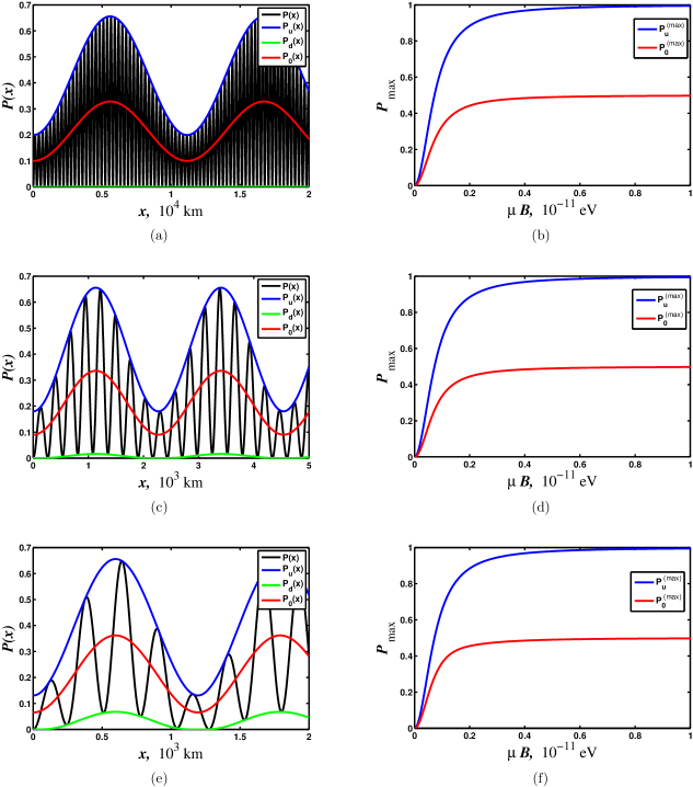
Figure 5: (color online) (a), (c) and (e) The transition probability versus the distance passed by a neutrino beam. The neutrino parameters have the same values as in Figs. 2-4, $E_{\nu}=10\thinspace\text{MeV}$, $\delta m^{2}=8\times 10^{-5}\thinspace\text{eV}^{2}$ and $\theta=0.6$. The magnetic energy is equal to $\mu B=10^{-12}\thinspace\text{eV}$. The black line is the function $P(x)$, the blue and green lines are the envelope functions $P_{u,d}(x)$ and the red line is the averaged transition probability $P_{0}(x)$. (b), (d) and (f) The dependence of the maximal values of the functions $P(x)$ and $P_{0}(x)$, blue and red lines respectively, on the magnetic energy for the given density. Panels (a) and (b) correspond to the matter density $\rho=10\thinspace\text{g/cc}$, (c) and (d) to $\rho=50\thinspace\text{g/cc}$ and (e) and (f) to $\rho=100\thinspace\text{g/cc}$. This figure is taken from Ref. DvoMaa09 .

Despite the formal similarity between Dirac and Majorana transition probabilities [see Eqs. (VI) and (X)] the actual dynamics is quite different in these two cases, as one can see by comparing Figs. 2(d)-4(d) and Fig. 5, panels (b), (d) and (f). In particular, in the Majorana case $P_{u}^{\mathrm{(max)}}=4|C_{+{}}C_{-{}}|$ for arbitrary $B$, to be compared with Eq. (93), while the function $P_{0}^{\mathrm{(max)}}$ has the same form as in the Dirac case given in Eq. (94). In contrast with the Dirac case, the averaged transition probability does not achieve its maximal value at some moderate magnetic field $B_{\mathrm{max}}$ value, but both $P_{u}^{\mathrm{max}}$ and $P_{0}^{\mathrm{max}}$ are monotonically increasing functions of the strength of the magnetic field with 1 and 1/2 as their asymptotic values, respectively. We can understand this behavior when we recall that, at $\mu B\gg\max(\Phi,V)$, the effective Hamiltonian Eq. (118) becomes

$$H_{\infty}=\mathrm{i}\mu B\gamma^{2},\quad\mathrm{i}\gamma^{2}=\begin{pmatrix}0&0&0&1\\ 0&0&-1&0\\ 0&-1&0&0\\ 1&0&0&0\ \end{pmatrix}.$$ (126)

The Schrödinger equation with the effective Hamiltonian (126) has the formal solution

$$\Psi(t)=\exp(-\mathrm{i}H_{\infty}t)\Psi(0)=[\cos(\mu Bt)+\gamma^{2}\sin(\mu Bt)]\Psi(0).$$ (127)

Using Eqs. (98), (125) and (127) we then immediately arrive to the following expression for the transition probability, $P(t)=|\nu_{\alpha}^{\mathrm{R}}|^{2}=\sin^{2}(\mu Bt)$, which explains the behavior of the function $P_{u}^{\mathrm{(max)}}$ at strong magnetic fields. Note that the analogous result was also obtained in Ref. LikStu95 .

Finally, it is worth of noticing that in contrast to the Dirac case, the behavior of the transition probability in the Majorana case is qualitatively similar for different matter densities and different magnetic fields [see Fig. 5, panels (a), (c), and (e)].

The problem of Majorana neutrinos’ spin flavor oscillations was studied in Refs. AndSatPRD03 ; AndSatJCAP03 with help of numerical codes. For example, in Ref. AndSatPRD03 the evolution equation for three neutrino flavors propagating inside a presupernova star with zero metallicity, e.g., corresponding to W02Z model WooHegWea02 , was solved for the realistic matter and magnetic field profiles. Although our analytical transition probability formula (X) is valid only for the constant matter density and magnetic field strength, it is interesting to compare our results with the numerical simulations of Ref. AndSatPRD03 . In those calculations the authors used magnetic fields $B\sim 10^{10}\thinspace\text{G}$ and magnetic moments $\sim 10^{-12}\thinspace\mu_{\mathrm{B}}$ that give us the magnetic energy $\mu B\sim 10^{-11}\thinspace\text{eV}$. This value is the maximal magnetic energy used in our work.

It was found in Ref. AndSatPRD03 that spin flavor conversion is practically adiabatic for low-energy neutrinos corresponding to $E_{\nu}\sim 5\thinspace\text{MeV}$ inside the region where $Y_{e}\approx 0.5$ and the averaged transition probability for the channel $\nu_{\mu}\to\bar{\nu}_{e}$ is close $0.5$. This big transition probability is due to the RSF-H and RSF-L resonances at the distance $\approx 0.01R_{\odot}$. Even so that we study two neutrino oscillations scheme, we obtained the analogous behavior of $P_{0}^{\mathrm{(max)}}$ (see Fig. 5). However, in our case this big transition probability is due to the presence of the strong magnetic field (see Refs. GiuStu09 ; LikStu95 ). We cannot compare our transition probability formula (X) with the results of Ref. AndSatPRD03 for higher energies, $E_{\nu}>25\thinspace\text{MeV}$, since spin flavor oscillations become strongly nonadiabatic for these kinds of energies and one has to take into account the coordinate dependence of the matter density which should decrease with radius as $1/r^{3}$ Kac02 .

XI Evolution of neutrinos emitted by classical sources

In this section we present an alternative approach to the description of neutrino flavor oscillations which involves the studies of the evolution of mixed massive neutrinos in vacuum under the influence of external classical fields Dvo09 . These fields are supposed to be localized in space and treated as “sources” which emit flavor neutrinos.

As in Secs. II-V we consider a number of flavor neutrinos $\nu_{\lambda}$, which, in principle, can be arbitrary: $\lambda=e,\mu,\tau,\dotsc$. Note that we will formulate the dynamics of the system in terms of the left $\nu_{\lambda}^{\mathrm{L}}$ and right $\nu_{\lambda}^{\mathrm{R}}$ handed chiral components of the neutrino spinors.

The external sources are denoted as $J_{\lambda}^{\mu}$. It should be noted that, if one describes the emission of mixed massive neutrinos in any process within the quantum field theory, there is a nonzero probability of emission of neutrinos of different flavors Shr80 . Although a source of one particular flavor can prevail, one should always consider the situation when the sources of all flavors are present.

The Lorentz invariant Lagrangian describing the evolution of this system has the form,

$$\mathcal{L}= \sum_{\lambda}\left(\overline{\nu_{\lambda}^{\mathrm{L}}}\mathrm{i}\gamma^{\mu}\partial_{\mu}\nu_{\lambda}^{\mathrm{L}}+\overline{\nu_{\lambda}^{\mathrm{R}}}\mathrm{i}\gamma^{\mu}\partial_{\mu}\nu_{\lambda}^{\mathrm{R}}\right)$$

$$-\sum_{\lambda\lambda^{\prime}}\Big{(}m_{\lambda\lambda^{\prime}}^{\mathrm{D}}\overline{\nu_{\lambda}^{\mathrm{L}}}\nu_{\lambda^{\prime}}^{\mathrm{R}}+m_{\lambda\lambda^{\prime}}^{\mathrm{L}}\left(\nu_{\lambda}^{\mathrm{L}}\right)^{\mathrm{T}}C\nu_{\lambda^{\prime}}^{\mathrm{L}}$$

$$+m_{\lambda\lambda^{\prime}}^{\mathrm{R}}\left(\nu_{\lambda}^{\mathrm{R}}\right)^{\mathrm{T}}C\nu_{\lambda^{\prime}}^{\mathrm{R}}+\text{h.c.}\Big{)}$$

$$+\sum_{\lambda}\left(\overline{\nu_{\lambda}^{\mathrm{L}}}\gamma_{\mu}\ell_{\lambda}^{\mathrm{L}}J_{\lambda}^{\mu}+\text{h.c.}\right),$$ (128)

where $\left(m_{\lambda\lambda^{\prime}}^{\mathrm{D}}\right)$, $\left(m_{\lambda\lambda^{\prime}}^{\mathrm{L}}\right)$, $\left(m_{\lambda\lambda^{\prime}}^{\mathrm{R}}\right)$ are the Dirac as well as (left and right) Majorana mass matrices and $C=\mathrm{i}\gamma^{2}\gamma^{0}$ is the charge conjugation matrix. These mass matrices should satisfy certain requirements which are discussed in Ref. Kob80 . The Lagrangian (XI) is CPT-invariant. In this section we adopt the notations for Dirac matrices as in Ref. ItzZub84p385 . The analogous mass terms are generated in theoretical models based on the type-II seesaw mechanism (see, e.g., Ref. SchVal80 ).

The external fields $J_{\lambda}^{\mu}=J_{\lambda}^{\mu}(\mathbf{r},t)$ can be arbitrary functions. If we suppose that neutrinos interact with external sources in frames of the electroweak model, the spinor $\ell_{\lambda}$ in Eq. (XI) is the charged $\mathrm{SU}(2)$ isodoublet partner of $\nu_{\lambda}$. For example, we can study the neutrino emission in a process like the inverse $\beta$-decay: $p+e^{-}\to\nu_{e}+n$. In this case the external fields in Eq. (XI) are (see, e.g., Ref. Oku90p36 )

$$J_{\nu_{e}}^{\mu}= -\sqrt{2}G_{\mathrm{F}}\bar{\varPsi}_{n}\gamma^{\mu}(1-\alpha\gamma^{5})\varPsi_{p},$$

$$J_{\nu_{\mu}}^{\mu}= 0,\quad J_{\nu_{\tau}}^{\mu}=0,$$ (129)

where $\varPsi_{p}$ and $\varPsi_{n}$ are the wave functions of a proton and a neutron, $\alpha\approx 1.25$. In Eq. (XI) we assume that a source consists of electrons, protons and neutrons.

To proceed in the analysis of the dynamics of the system (XI) we should diagonalize the mass term of the Lagrangian. The diagonalized Lagrangian is expressed in terms of the Majorana fields with different masses Kob80 . In general case the number of these Majorana fields is double than the number of flavors in the initial Lagrangian. In the following we discuss the case when only Dirac mass term is presented. Then we study the general situation.

XI.1 Dirac mass term

In this section we suppose that only Dirac mass matrix is present in Eq. (XI). Analogously to the discussion in Sec. II we introduce the new set of spinor fields $\psi_{a}$. In our situation the mixing matrix is a square unitary matrix $(U_{\lambda a})$,

$$\nu_{\lambda}=\sum_{a}U_{\lambda a}\psi_{a}.$$ (130)

By definition the mass eigenstates $\psi_{a}$ are Dirac particles.

When we transform the Lagrangian (XI) using Eq. (130), it is rewritten in the following way:

$$\mathcal{L}=\sum_{a}\bar{\psi}_{a}(\mathrm{i}\gamma^{\mu}\partial_{\mu}-m_{a})\psi_{a}+\sum_{a}(\bar{\psi}_{a}\xi_{a}+\text{h.c.}),$$ (131)

where $\xi_{a}$ is the external source for the fermion $\psi_{a}$,

$$\xi_{a}=\sum_{\lambda}U_{a\lambda}^{\dagger}\gamma_{\mu}^{\mathrm{L}}\ell_{\lambda}f_{\lambda}^{\mu}.$$ (132)

Using Eqs. (131) and (132) we receive the inhomogeneous Dirac equation for the fermion $\psi_{a}$,

$$(\mathrm{i}\gamma^{\mu}\partial_{\mu}-m_{a})\psi_{a}=-\xi_{a}.$$ (133)

As in Sec. II the masses $m_{a}$ are the eigenvalues of the matrix $(m_{\lambda\lambda^{\prime}}^{\mathrm{D}})$.

The solution to Eq. (132) for the arbitrary spinor $\xi_{a}$ is expressed with help of the retarded Green function for a spinor field (see Ref. BogShi80p140 ),

$$\psi_{a}(\mathbf{r},t)=\int\mathrm{d}^{3}\mathbf{r}^{\prime}\mathrm{d}t^{\prime}S^{\mathrm{ret}}_{a}(\mathbf{r}-\mathbf{r}^{\prime},t-t^{\prime})\xi_{a}(\mathbf{r}^{\prime},t^{\prime}).$$ (134)

The explicit form of $S^{\mathrm{ret}}_{a}(\mathbf{r},t)$ can be also found in Ref. BogShi80p140 ,

$$S^{\mathrm{ret}}_{a}(\mathbf{r},t)=(\mathrm{i}\gamma^{\mu}\partial_{\mu}+m_{a})D^{\mathrm{ret}}_{a}(\mathbf{r},t).$$ (135)

In Eq. (135) $D^{\mathrm{ret}}_{a}(\mathbf{r},t)$ is the retarded Green function for a scalar field BogShi80p140 ,

$$D^{\mathrm{ret}}_{a}(\mathbf{r},t)= \int\frac{\mathrm{d}^{4}p}{(2\pi)^{4}}\frac{e^{\mathrm{i}px}}{m_{a}^{2}-p^{2}+\mathrm{i}\epsilon p^{0}}$$

$$= \frac{1}{2\pi}\theta(t)\left\{\delta(s^{2})-\theta(s^{2})\frac{m_{a}}{2s}J_{1}(m_{a}s)\right\},$$ (136)

where $\theta(t)$ is the Heaviside step function, $J_{1}(z)$ is the first order Bessel function, $s=\sqrt{t^{2}-r^{2}}$ and $r=|\mathbf{r}|$.

To proceed in further calculations it is necessary to define the behavior of the external sources. We assume that the sources are localized in space and emit harmonic radiation,

$$\ell_{\lambda}(\mathbf{r},t)J_{\lambda}^{\mu}(\mathbf{r},t)=\theta(t)l_{\lambda}J_{\lambda}^{(0)\mu}e^{-\mathrm{i}Et}\delta^{3}(\mathbf{r}),$$ (137)

where $l_{\lambda}=\ell^{(0)}_{\lambda}$ is the time independent component of the spinor $\ell_{\lambda}$, $J_{\lambda}^{(0)\mu}$ is the amplitude of the function $J_{\lambda}^{\mu}(\mathbf{r},t)$, and $E$ is the frequency of the source. Using Eqs. (132) and (137) we obtain for $\xi_{a}$,

$$\xi_{a}(\mathbf{r},t)= \theta(t)\xi_{a}^{(0)}e^{-\mathrm{i}Et}\delta^{3}(\mathbf{r}),$$

$$\xi_{a}^{(0)}= \sum_{\lambda}U_{a\lambda}^{\dagger}\gamma_{\mu}^{\mathrm{L}}l_{\lambda}J_{\lambda}^{(0)\mu}.$$ (138)

With help of Eqs. (135)-(XI.1) we can rewrite Eq. (134) in the following way:

$$\psi_{a}(\mathbf{r},t)= \left(\mathrm{i}\gamma^{\mu}\frac{\partial}{\partial x^{\mu}}+m_{a}\right)$$

$$\times\left\{e^{-\mathrm{i}Et}\int_{0}^{t}\mathrm{d}\tau D^{\mathrm{ret}}_{a}(\mathbf{r},\tau)e^{\mathrm{i}E\tau}\right\}\xi_{a}^{(0)}.$$ (139)

One can see that two major terms appear in Eq. (XI.1) [see also Eq. (XI.1)] while integrating over $\tau$

$$\int_{0}^{t}\mathrm{d}\tau D^{\mathrm{ret}}_{a}(\mathbf{r},\tau)e^{\mathrm{i}E\tau}=\mathcal{I}_{1}+\mathcal{I}_{2}.$$ (140)

They are

$$\mathcal{I}_{1} =\frac{1}{2\pi}\int_{0}^{t}\mathrm{d}\tau\delta(s^{2})e^{\mathrm{i}E\tau}=\frac{\theta(t-r)}{4\pi r}e^{\mathrm{i}Er},$$ (141)

$$\mathcal{I}_{2} =-\frac{m_{a}}{4\pi}\int_{0}^{t}\mathrm{d}\tau\theta(s^{2})\frac{J_{1}(m_{a}s)}{s}e^{\mathrm{i}E\tau}$$

$$=-\frac{m_{a}}{4\pi}\theta(t-r)\int_{0}^{x_{m}}\mathrm{d}x\frac{J_{1}(m_{a}x)}{\sqrt{r^{2}+x^{2}}}e^{\mathrm{i}E\sqrt{r^{2}+x^{2}}},$$ (142)

where $x_{m}=\sqrt{t^{2}-r^{2}}$ and $s=\sqrt{\tau^{2}-r^{2}}$. It is interesting to notice that both $\mathcal{I}_{1}$ and $\mathcal{I}_{2}$ in Eqs. (141) and (XI.1) are equal to zero if $t<r$. It means that the initial perturbation from a source placed at the point $\mathbf{r}=0$ reaches a detector placed at the point $\mathbf{r}$ only after the time $t>r$.

Despite the integral $\mathcal{I}_{1}$ in Eq. (141) is expressed in terms of the elementary functions, the integral $\mathcal{I}_{2}$ in Eq. (XI.1) cannot be computed analytically for arbitrary $r$ and $t$. However some reasonable assumptions can be made to simplify the considered expression. Suppose that an observer is at the fixed distance from a source. As we have already mentioned one detects a signal starting from $t>r$. It is obvious that a nonstationary rapidly oscillating signal is detected when the wave front just arrives to a detector, i.e. when $t\gtrsim r$. The situation is analogous to waves propagating on the water surface. Therefore, if we suppose that one starts observing particles when the non-stationary signal attenuates, i.e. $t\gg r$ or $x_{m}\to\infty$, we can avoid relaxation phenomena. In this case the integral $\mathcal{I}_{2}$ can be computed analytically,

$$\mathcal{I}_{2}=-\frac{1}{4\pi r}(e^{\mathrm{i}Er}-e^{\mathrm{i}p_{a}r}),$$ (143)

where $p_{a}=\sqrt{E^{2}-m_{a}^{2}}$ is the analog of the particle momentum.

To obtain Eq. (143) we use the known values of the integrals,

$$\int_{0}^{\infty}\mathrm{d}x \frac{J_{\nu}(mx)}{\sqrt{r^{2}+x^{2}}}\sin(E\sqrt{r^{2}+x^{2}})$$

$$= \frac{\pi}{2}J_{\nu/2}\left[\frac{r}{2}\left(E-\sqrt{E^{2}-m^{2}}\right)\right]$$

$$\times J_{-\nu/2}\left[\frac{r}{2}\left(E+\sqrt{E^{2}-m^{2}}\right)\right],$$

$$\int_{0}^{\infty}\mathrm{d}x \frac{J_{\nu}(mx)}{\sqrt{r^{2}+x^{2}}}\cos(E\sqrt{r^{2}+x^{2}})$$

$$= -\frac{\pi}{2}J_{\nu/2}\left[\frac{r}{2}\left(E-\sqrt{E^{2}-m^{2}}\right)\right]$$

$$\times N_{-\nu/2}\left[\frac{r}{2}\left(E+\sqrt{E^{2}-m^{2}}\right)\right],$$ (144)

and the fact that the Bessel and Neumann functions of $\pm 1/2$ order

$$J_{1/2}(z)= N_{-1/2}(z)=\sqrt{\frac{2}{\pi z}}\sin z,$$

$$J_{-1/2}(z)= \sqrt{\frac{2}{\pi z}}\cos z,$$ (145)

are expressed in terms of the elementary functions. The approximations made in derivation of Eq. (143) are analysed in Appendix C.

Using Eqs. (XI.1)-(XI.1) we obtain the field distribution of the fermion $\psi_{a}$ in the following form:

$$\psi_{a}(\mathbf{r},t)=e^{-\mathrm{i}Et+\mathrm{i}p_{a}r}O_{a}\frac{\xi_{a}^{(0)}}{4\pi r},$$ (146)

where $O_{a}=\gamma^{0}E-(\bm{\gamma}\mathbf{n})p_{a}+m_{a}$ and $\mathbf{n}$ is the unit vector towards a detector. It should be noted that in deriving Eq. (146) we differentiate only exponential rather than the factor $1/r$ because the derivative of $1/r$ is proportional to $1/r^{2}$. Such a term is negligible at large distances from a source. We also remind that Eq. (146) is valid for $t\gg r$.

Let us turn to the description of the evolution of the fields $\nu_{\lambda}$. Using Eqs. (130) and (146), we obtain the corresponding wave function,

$$\nu_{\lambda}(\mathbf{r},t)=e^{-\mathrm{i}Et}\sum_{a\lambda^{\prime}}U_{\lambda a}U_{a\lambda^{\prime}}^{\dagger}e^{\mathrm{i}p_{a}r}O_{a}\gamma_{\mu}^{\mathrm{L}}l_{\lambda^{\prime}}\frac{J_{\lambda^{\prime}}^{(0)\mu}}{4\pi r}.$$ (147)

As in Secs. II-V we study the evolution of only two fermions. The mixing matrix is given in Eq. (4). We also choose the amplitudes of the sources in the following way: $J_{\alpha}^{(0)\mu}=0$, $J_{\beta}^{(0)\mu}\equiv J^{\mu}\neq 0$ and $l_{\beta}\equiv l$. This choice of the sources corresponds to the emission of neutrinos of the flavor “$\beta$” and detection of the neutrinos belonging to the flavor “$\alpha$” at the distance $r$ from a source. Using Eqs. (4) and (147) we obtain the wave functions of each of the particles $\nu_{\alpha,\beta}$,

$$\nu_{\alpha}(\mathbf{r},t)= \sin\theta\cos\theta e^{-\mathrm{i}Et}\frac{J^{\mu}}{4\pi r}$$

$$\times(e^{\mathrm{i}p_{1}r}O_{1}-e^{\mathrm{i}p_{2}r}O_{2})\gamma_{\mu}^{\mathrm{L}}l,$$

$$\nu_{\beta}(\mathbf{r},t)= e^{-\mathrm{i}Et}\frac{J^{\mu}}{4\pi r}$$

$$\times(\sin^{2}\theta e^{\mathrm{i}p_{1}r}O_{1}+\cos^{2}\theta e^{\mathrm{i}p_{2}r}O_{2})\gamma_{\mu}^{\mathrm{L}}l.$$ (148)

In the following we discuss the high frequency approximation, $E\gg m_{1,2}$, which corresponds to the emission of ultrarelativistic neutrinos.

The probability to detect a neutrino of the flavor “$\lambda$” can be calculated as $P_{\lambda}(\mathbf{r},t)=|\nu_{\lambda}(\mathbf{r},t)|^{2}$. Finally using Eq. (XI.1) we get for the probabilities,

$$P_{\alpha}(r)= -2E^{2}\frac{J^{{\dagger}\mu}J^{\nu}}{(4\pi r)^{2}}\langle T_{\mu\nu}\rangle$$

$$\times\left\{\sin^{2}(2\theta)\sin^{2}\left(\frac{\delta m^{2}}{4E}r\right)+\mathcal{O}\left(\frac{m_{a}^{2}}{E^{2}}\right)\right\},$$

$$P_{\beta}(r)= -2E^{2}\frac{J^{{\dagger}\mu}J^{\nu}}{(4\pi r)^{2}}\langle T_{\mu\nu}\rangle$$

$$\times\bigg{\{}1-\sin^{2}(2\theta)\sin^{2}\left(\frac{\delta m^{2}}{4E}r\right)$$

$$+\mathcal{O}\left(\frac{m_{a}^{2}}{E^{2}}\right)\bigg{\}},$$ (149)

where $\langle T_{\mu\nu}\rangle=l^{\dagger}\gamma_{\mu}^{\dagger}(\bm{\alpha}\mathbf{n})\gamma_{\nu}l$. It is possible to calculate the components of the tensor $\langle T_{\mu\nu}\rangle$. They depend on the properties of the fermion $\ell_{\beta}\equiv\ell$,

$$\langle T_{00}\rangle=-(\mathbf{v}\mathbf{n}),\quad\langle T_{0i}\rangle=\langle T_{i0}\rangle^{*}=n_{i}-\mathrm{i}[\mathbf{n}\times\bm{\zeta}]_{i},$$

$$\langle T_{ij}\rangle=\delta_{ij}(\mathbf{v}\mathbf{n})-(v_{i}n_{j}+v_{j}n_{i})+\mathrm{i}\varepsilon_{ijk}n_{k},$$ (150)

where $\mathbf{v}=\langle\bm{\alpha}\rangle$ is the velocity of fermion $\ell$ and $\bm{\zeta}=\langle\bm{\Sigma}\rangle$ is its spin.

Let us discuss the simplified case when the spatial components of the four-vector $J^{\mu}$ are equal to zero: $\mathbf{J}=0$. It corresponds to the neutrino emission by a nonmoving and unpolarized source. Using Eqs. (XI.1) and (150) we can find the transition and survival probabilities in the following way:

$$P_{\beta\to\alpha}(r)\sim \sin^{2}(2\theta)\sin^{2}\left(\frac{\delta m^{2}}{4E}r\right),$$ (151)

$$P_{\beta\to\beta}(r)\sim 1-\sin^{2}(2\theta)\sin^{2}\left(\frac{\delta m^{2}}{4E}r\right),$$ (152)

where we drop the common factor $2E^{2}(\mathbf{v}\mathbf{n})|J^{0}|^{2}/(4\pi r)^{2}$ to have the probabilities normalized to unity. It should be noted that Eqs. (151) and (152) are the same as the common formulae for the description of neutrino flavor oscillations in vacuum Kob80 ; GriPon69 .

XI.2 General mass term

When both Dirac and Majorana mass matrices are present in Eq. (XI), left and right handed chiral components should be transformed independently (see also Ref. Kob80 ),

$$\nu_{\lambda}^{\mathrm{L}}=\sum_{a}U_{\lambda a}\Psi_{a}^{\mathrm{L}},\quad\nu_{\lambda}^{\mathrm{R}}=\sum_{a}V_{\lambda a}\Psi_{a}^{\mathrm{R}},$$ (153)

with help of the matrices $(U_{\lambda a})$ and $(V_{\lambda a})$ to diagonalize the general mass term. Note that these matrices are rectangular and nonhermitian. The modern parameterization for these matrices is given in Ref. Xin08 .

However one cannot say whether particles $\Psi_{a}^{\mathrm{L,R}}$ are Majorana or Dirac although they correspond to definite mass eigenstates. That is why we introduce a new field $\psi_{a}=\Psi_{a}^{\mathrm{L}}+(\Psi_{a}^{\mathrm{L}})^{c}$ which is Majorana by definition.

The Lagrangian for the particles $\psi_{a}$ takes the form,

$$\mathcal{L}= \sum_{a}\Big{(}\overline{\psi_{a}^{\mathrm{L}}}\mathrm{i}\gamma^{\mu}\partial_{\mu}\psi_{a}^{\mathrm{L}}-m_{a}\overline{\psi_{a}^{\mathrm{L}}}\psi_{a}^{\mathrm{R}}$$

$$+\overline{\psi_{a}^{\mathrm{L}}}\xi_{a}^{\mathrm{R}}+\text{h.c.}\Big{)},$$ (154)

where the external sources $\xi_{a}\equiv\xi_{a}^{\mathrm{R}}$ have the same form as in Eq. (132).

As we mentioned in Sec. VIII, Majorana spinors are equivalent to two component Weil spinors Cas57 . Hence we can rewrite the spinors $\psi_{a}^{\mathrm{L,R}}$ and $\xi_{a}$ as

$$\psi_{a}^{\mathrm{L}}=\begin{pmatrix}0\\ \eta_{a}\end{pmatrix},\quad\psi_{a}^{\mathrm{R}}=\begin{pmatrix}\mathrm{i}\sigma_{2}\eta_{a}^{*{}}\\ 0\end{pmatrix},\quad\xi_{a}=\begin{pmatrix}\phi_{a}\\ 0\end{pmatrix},$$ (155)

where

$$\phi_{a}=\sum_{\lambda}U_{a\lambda}^{\dagger}\chi_{\lambda}J_{\lambda}^{0}.$$ (156)

To obtain Eq. (156) we suppose that, as in Sec. XI.1, the vectors $J_{\lambda}^{\mu}$ have only time component $J_{\lambda}^{0}$. We also assume that $\left(\ell^{\mathrm{L}}_{\lambda}\right)^{\mathrm{T}}=(0,\chi_{\lambda})$. To derive Eq. (156) it is crucial that only left handed currents interactions are presented in Eq. (XI).

It is useful to rewrite the Lagrangian (XI.2) in terms of the two component spinors $\eta_{a}$ and $\phi_{a}$ FukYan03p292 ,

$$\mathcal{L}= \sum_{a}\mathrm{i}\eta_{a}^{\dagger}(\partial_{t}-\bm{\sigma}\bm{\nabla})\eta_{a}$$

$$+\sum_{a}\left(\frac{\mathrm{i}}{2}m_{a}\eta_{a}^{\dagger}\sigma_{2}\eta_{a}^{*{}}+\eta_{a}^{\dagger}\phi_{a}+\text{h.c.}\right).$$ (157)

Using Eq. (XI.2) we can receive the wave equation for two-component spinors,

$$\left(\frac{\partial}{\partial t}-\bm{\sigma}\bm{\nabla}\right)\eta_{a}+m_{a}\sigma_{2}\eta_{a}^{*{}}=\mathrm{i}\phi_{a}.$$ (158)

The solutions of Eq. (158) have the form (see, e.g., Ref. FukYan03p292 ),

$$\eta_{a}(\mathbf{r},t)=\int\mathrm{d}^{3}\mathbf{r}^{\prime}\mathrm{d}t^{\prime}\mathcal{S}^{\mathrm{ret}}_{a}(\mathbf{r}-\mathbf{r}^{\prime},t-t^{\prime})\phi_{a}(\mathbf{r}^{\prime},t^{\prime}),$$ (159)

$$\eta_{a}^{*{}}(\mathbf{r},t)=\int\mathrm{d}^{3}\mathbf{r}^{\prime}\mathrm{d}t^{\prime}\mathcal{R}^{\mathrm{ret}}_{a}(\mathbf{r}-\mathbf{r}^{\prime},t-t^{\prime})\phi_{a}(\mathbf{r}^{\prime},t^{\prime}),$$ (160)

where the retarded Green functions are expressed as (see also Ref. FukYan03p292 ),

$$\mathcal{S}_{a}^{\mathrm{ret}}(\mathbf{r},t)= \mathrm{i}\tilde{\sigma}^{\mu}\partial_{\mu}D_{a}^{\mathrm{ret}}(\mathbf{r},t),$$

$$\mathcal{R}_{a}^{\mathrm{ret}}(\mathbf{r},t)= \mathrm{i}m_{a}\sigma_{2}D_{a}^{\mathrm{ret}}(\mathbf{r},t).$$ (161)

Here $\partial_{\mu}=(\partial_{t},\bm{\nabla})$, $\tilde{\sigma}^{\mu}=(\sigma^{0},\bm{\sigma})$, $\sigma^{0}$ is the $2\times 2$ unit matrix, $\bm{\sigma}$ are Pauli matrices, and $D_{a}^{\mathrm{ret}}(\mathbf{r},t)$ is given in Eq. (XI.1). One can check that Eq. (159) and (160), along with the definition of the retarded Green functions (XI.2), represent the solutions to Eq. (158) by means of direct substituting.

Let us assume that the sources $\phi_{a}$ depend on time and spatial coordinates as in Sec. XI.1,

$$\phi_{a}(\mathbf{r},t)= \theta(t)\phi_{a}^{(0)}e^{-\mathrm{i}Et}\delta^{3}(\mathbf{r}),$$

$$\phi_{a}^{(0)}= \sum_{\lambda}U^{\dagger}_{a\lambda}J_{\lambda}\chi^{(0)}_{\lambda},$$ (162)

where $\chi^{(0)}_{\lambda}$ is the time independent component of $\chi_{\lambda}$. In deriving of Eq. (XI.2) from Eq. (156) we introduce the new quantities $J_{\lambda}\equiv J_{\lambda}^{(0)0}$, where $J_{\lambda}^{(0)0}$ is the time independent part of $J_{\lambda}^{0}$, to simplify the notations.

On the basis of Eqs. (159)-(XI.2) and using the technique developed in Sec. XI.1 we get the particles wave functions,

$$\eta_{a}(\mathbf{r},t)= \mathrm{i}\tilde{\sigma}^{\mu}\partial_{\mu}[e^{-\mathrm{i}Et+\mathrm{i}p_{a}r}]\frac{\phi_{a}^{(0)}}{4\pi r},$$ (163)

$$\eta_{a}^{*{}}(\mathbf{r},t)= \mathrm{i}m_{a}\sigma_{2}e^{-\mathrm{i}Et+\mathrm{i}p_{a}r}\frac{\phi_{a}^{(0)}}{4\pi r}.$$ (164)

To derive Eqs. (163) and (164) we suppose that $t\gg r$. The derivatives in Eq. (163) are applied on the exponent only because of the same reasons as in Sec. XI.1.

Using Eqs. (153), (163) and (164) as well as the following identity:

$$\left(\nu_{\lambda}^{\mathrm{L}}\right)^{c}= \left(\nu_{\lambda}^{c}\right)^{\mathrm{R}}=\sum_{a}U_{\lambda a}^{*{}}\psi_{a}^{\mathrm{R}},$$

$$\left(\nu_{\lambda}^{\mathrm{L}}\right)^{c}= C\left(\overline{\nu_{\lambda}^{\mathrm{L}}}\right)^{\mathrm{T}},$$ (165)

we get the wave functions of $\nu_{\lambda}^{\mathrm{L}}$ and $\left(\nu_{\lambda}^{\mathrm{L}}\right)^{c}$ as

$$\nu_{\lambda}^{\mathrm{L}}(\mathbf{r},t)= \frac{2E}{4\pi r}e^{-\mathrm{i}Et}\sum_{a\lambda^{\prime}}e^{\mathrm{i}p_{a}r}U_{\lambda a}U_{a\lambda^{\prime}}^{\dagger}$$

$$\times J_{\lambda^{\prime}}\begin{pmatrix}0\\ \tilde{\chi}^{(0)}_{\lambda^{\prime}}\end{pmatrix},$$ (166)

$$\left(\nu_{\lambda}^{\mathrm{L}}\right)^{c}(\mathbf{r},t)= -\frac{2E}{4\pi r}e^{-\mathrm{i}Et}\sum_{a\lambda^{\prime}}\frac{m_{a}}{2E}e^{\mathrm{i}p_{a}r}U_{\lambda a}^{*{}}U_{a\lambda^{\prime}}^{\dagger}$$

$$\times J_{\lambda^{\prime}}\begin{pmatrix}\chi^{(0)}_{\lambda^{\prime}}\\ 0\end{pmatrix},$$ (167)

where $\tilde{\chi}^{(0)}_{\lambda^{\prime}}=(1/2)[1-(\bm{\sigma}\mathbf{n})]\chi^{(0)}_{\lambda^{\prime}}$. In deriving of Eq. (XI.2) we suppose that

$$[E-p_{a}(\bm{\sigma}\mathbf{n})]\approx E[1-(\bm{\sigma}\mathbf{n})],$$ (168)

that is valid for relativistic neutrinos.

It is possible to construct two four component Majorana spinors from two-component Weil spinors,

$$\psi_{a}^{(1)}=\begin{pmatrix}\mathrm{i}\sigma_{2}(\eta_{a})^{*{}}\\ \eta_{a}\end{pmatrix},\quad\psi_{a}^{(2)}=\begin{pmatrix}\mathrm{i}\sigma_{2}\eta_{a}^{*{}}\\ (\eta_{a}^{*{}})^{*{}}\end{pmatrix},$$ (169)

where $\eta_{a}$ and $\eta_{a}^{*{}}$ are defined in Eqs. (163) and (164). One can see that these spinors satisfy the Majorana condition $\left[\psi_{a}^{(1,2)}\right]^{c}=\psi_{a}^{(1,2)}$. We use the spinor $\psi_{a}^{(1)}$ to receive Eq. (XI.2) and $\psi_{a}^{(2)}$ for Eq. (XI.2). In this case we get that $\nu_{\lambda}^{\mathrm{L}}$ and $\left(\nu_{\lambda}^{\mathrm{L}}\right)^{c}$ are obtained as a result of the evolution of particles emitted from the same source.

It should be mentioned that both $\nu_{\lambda}^{\mathrm{L}}$ and $\left(\nu_{\lambda}^{\mathrm{L}}\right)^{c}$ in Eqs. (XI.2) and (XI.2) propagate forward in time. To explain this fact let us discuss the complex conjugated equation (159). Performing the same computations one arrives to the analog of Eq. (XI.2) which would depend on time as $e^{\mathrm{i}Et}$. However this wave function describes a particle emitted by the source different from that discussed here. Indeed, if we studied the complex conjugated Eq. (159), the integrand there would be $\mathcal{S}^{\mathrm{ret*{}}}_{a}\phi_{a}^{*{}}$. It would mean that the source in Eq. (XI.2) would be proportional to $\phi_{a}^{(0)*{}}e^{\mathrm{i}Et}$, that, in its turn, would signify that $\left(\nu_{\lambda}^{\mathrm{L}}\right)^{c}$ would be emitted in a process involving a lepton which is a charge conjugated counterpart to that discussed here.

Let us illustrate this problem on a more physical example. Suppose that we study a neutrino emission in a process like the inverse $\beta$-decay,

$$p+\ell_{\lambda}^{-{}}\to n+\nu_{\lambda}\Rightarrow n+\sum_{a}U_{\lambda a}\psi_{a}^{\mathrm{L}},$$ (170)

where $p$, $n$ and $\ell_{\lambda}^{-{}}$ stand for a proton, a neutron and for a negatively charged lepton. The complex conjugated Eq. (159) would correspond to a process,

$$n+\ell_{\lambda}^{+{}}\to p+\tilde{\nu}_{\lambda}\Rightarrow p+\sum_{a}U_{\lambda a}^{*{}}\left(\psi_{a}^{\mathrm{L}}\right)^{c}$$

$$\Rightarrow p+\sum_{a}U_{\lambda a}^{*{}}\psi_{a}^{\mathrm{R}},$$ (171)

where $\tilde{\nu}_{\lambda}$ and $\ell_{\lambda}^{+{}}$ denote an antineutrino and a positively charged lepton, which is the charge conjugated counterpart to $\ell_{\lambda}^{-{}}$. In Eq. (XI.2) we use the facts that only left handed interactions exist in nature and the fields $\psi_{a}$ describe Majorana particles. As one can see, Eqs. (170) and (XI.2) represent two different processes. Hence, if we used $(\eta_{a})^{*{}}$ to obtain $\left(\nu_{\lambda}^{\mathrm{L}}\right)^{c}(\mathbf{r},t)$, i.e. after a beam of neutrinos passes some distance $r$, it would correspond to the initial reaction (XI.2) rather than (170). Note that the same result also follows from Eq. (169) if we replace $\psi_{a}^{(1)}\leftrightarrow\psi_{a}^{(2)}$ there.

Let us suppose for simplicity that the momentum of the fermion $\ell_{\lambda}$ is parallel to the neutrino momentum. It takes place if a relativistic incoming lepton is studied. We also assume that this fermion is in a state with the definite helicity,

$$\frac{1}{2}[1-(\bm{\sigma}\mathbf{n})]\chi^{(0)}_{\lambda}=\chi^{(0)}_{\lambda}.$$ (172)

This expression is again natural for the relativistic fermion $\ell_{\lambda}$. One can notice that the Lagrangian (XI) is written in terms of the left handed chiral projections of $\ell_{\lambda}$. Therefore, if we study a relativistic lepton, it will have its spin directed oppositely to the particle momentum as one can see from Eq. (172).

Using Eqs. (XI.2), (XI.2) and (172) as well as the orthonormality of the two-component spinors $\chi^{(0)}_{\lambda}$, $\left(\chi^{(0){\dagger}}_{\lambda}\chi^{(0)}_{\lambda^{\prime}}\right)=\delta_{\lambda\lambda^{\prime}}$, we get the probabilities to detect $\nu_{\lambda}^{\mathrm{L}}$ and $\left(\nu_{\lambda}^{\mathrm{L}}\right)^{c}$ as

$$P_{\nu_{\lambda}^{\mathrm{L}}}(r)\sim \sum_{ab,\lambda^{\prime}}e^{\mathrm{i}(p_{a}-p_{b})r}$$

$$\times U_{\lambda a}U_{a\lambda^{\prime}}^{\dagger}U_{b\lambda}^{\dagger}U_{\lambda^{\prime}b}|J_{\lambda^{\prime}}|^{2},$$ (173)

$$P_{\left(\nu_{\lambda}^{\mathrm{L}}\right)^{c}}(r)\sim \sum_{ab,\lambda^{\prime}}\frac{m_{a}m_{b}}{(2E)^{2}}e^{\mathrm{i}(p_{a}-p_{b})r}$$

$$\times U_{\lambda a}^{*{}}U_{a\lambda^{\prime}}^{\dagger}U_{b\lambda}^{\mathrm{T}}U_{\lambda^{\prime}b}|J_{\lambda^{\prime}}|^{2}.$$ (174)

In Eqs. (XI.2) and (XI.2) we drop the factor $(2E)^{2}/(4\pi r)^{2}$.

We can see that Eqs. (XI.2) and (XI.2) contain the oscillating exponent. This our result reproduces the usual formulae for neutrino oscillations in vacuum Kob80 . It should be also noticed that the expressions for the probabilities depend on $r$ rather than on $t$ in contrast to our previous works Dvo05 ; Dvo06 ; Dvo08JPCS ; DvoMaa07 ; Dvo10 ; Dvo08JPG ; DvoMaa09 . Note that the problem whether neutrino oscillations happen in space or in time was also discussed in Ref. AkhSmi09 . The similar coordinate dependence of the probabilities was obtained in Refs. Kob82 ; GiuKimLeeLee93 where the problem of neutrino oscillations in vacuum was studied.

It was mentioned in Ref. Kob82 that oscillations between active and sterile neutrinos are possible in case of the nonunitary matrix $(U_{\lambda a})$, i.e. the presence of only Majorana mass terms is not sufficient for the existence of this kind of transitions. The situation is analogous to that considered in the pioneering work PontecorvoOsc where oscillations between neutrinos and antineutrinos were studied. In Eq. (XI.2) we obtain that the probability to detect $\left(\nu_{\lambda}^{\mathrm{L}}\right)^{c}$ is suppressed by the factor $m_{a}m_{b}/E^{2}$. It is in agreement with the results of Refs. Kob82 ; SchVal81v23 as well as with Eq. (VIII).

XII Quantum field theory description of neutrino oscillations in background matter

In the present section we study neutrino oscillations in background matter (see Sec. III) in frames of the quantum field theory approach. In particular we will be interested to examine the influence of background matter on the transitions between neutrinos and antineutrinos discussed in Secs. VIII and XI.2.

Despite we could receive satisfactory results for the description of neutrino-to-antineutrino transitions in vacuum in frames of the relativistic quantum mechanics approach [see Eqs. (VIII) and (XI.2)] the accurate treatment of this process has to be done within the quantum field theory because of the following reason. For the case of Majorana neutrinos, particles are identical to their antiparticles and only in frames of the quantum field theory one has the most accurate description of antiparticle states. Moreover, as we have seen in Sec. VIII, “antineutrino” states appear along with the small factor $m_{a}/E_{\nu}$. Typically various approaches to the description of neutrino oscillations give contradictory results at this order of accuracy Beu02 . That is why we will use the quantum field theory treatment to capture such a tiny effect.

As in Sec. XI, we will study the system of flavor neutrinos $\nu_{\lambda}$, $\lambda=e,\mu,\tau,\dotsc$, propagating in dense background matter between two spatial points, $\mathbf{x}_{1}$ and $\mathbf{x}_{2}$. We suggest that emission and absorption of neutrinos is due to the interaction with leptons $l_{\lambda}^{\pm{}}$ and heavy nucleons $N$. i.e these interactions are localized in two spatial regions: a “source” and a “detector”. On the contrary, the neutrino interaction with background matter is uniformly distributed along the total neutrino propagation distance $\mathbf{L}=\mathbf{x}_{2}-\mathbf{x}_{1}$.

In general case the dynamics of the system of mixed massive neutrinos should be formulated in frames of the left $\nu_{\lambda}^{\mathrm{L}}$ and right $\nu_{\lambda}^{\mathrm{R}}$ handed projections of flavor neutrinos [see also Eq. (XI)],

$$\mathcal{L}= \sum_{\lambda}\left(\overline{\nu_{\lambda}^{\mathrm{L}}}\mathrm{i}\gamma^{\mu}\partial_{\mu}\nu_{\lambda}^{\mathrm{L}}+\overline{\nu_{\lambda}^{\mathrm{R}}}\mathrm{i}\gamma^{\mu}\partial_{\mu}\nu_{\lambda}^{\mathrm{R}}\right)$$

$$-\sum_{\lambda\lambda^{\prime}}\Big{(}m_{\lambda\lambda^{\prime}}^{\mathrm{D}}\overline{\nu_{\lambda}^{\mathrm{L}}}\nu_{\lambda^{\prime}}^{\mathrm{R}}+m_{\lambda\lambda^{\prime}}^{\mathrm{L}}\left(\nu_{\lambda}^{\mathrm{L}}\right)^{\mathrm{T}}C\nu_{\lambda^{\prime}}^{\mathrm{L}}$$

$$+m_{\lambda\lambda^{\prime}}^{\mathrm{R}}\left(\nu_{\lambda}^{\mathrm{R}}\right)^{\mathrm{T}}C\nu_{\lambda^{\prime}}^{\mathrm{R}}+\text{h.c.}\Big{)}$$

$$-\sum_{\lambda}\overline{\nu_{\lambda}^{\mathrm{L}}}\gamma_{\mu}\nu_{\lambda^{\prime}}^{\mathrm{L}}f_{\lambda\lambda^{\prime}}^{\mu}-\sqrt{2}G_{\mathrm{F}}\left(j^{\mu}J_{\mu}+\text{h.c.}\right),$$ (175)

where $m_{\lambda\lambda^{\prime}}^{\mathrm{D}}$ and $m_{\lambda\lambda^{\prime}}^{\mathrm{L,R}}$ are Dirac and Majorana mass matrices defined in Sec. XI, and

$$j^{\mu}=\sum_{\lambda}\overline{\nu_{\lambda}^{\mathrm{L}}}\gamma^{\mu}l_{\lambda}^{\mathrm{L}},$$ (176)

is the neutrino-lepton current. The effective potential of the neutrino interaction with background matter $f_{\lambda\lambda^{\prime}}^{\mu}$ [see Eq. (III)] is supposed to be coordinate independent, whereas the nuclear current $J_{\mu}$ is localized in space. We will take into account the interaction with background matter exactly. As in Sec. III here we study the general case and consider the matrix $(f_{\lambda\lambda^{\prime}}^{\mu})$ to be nondiagonal. Note that in Eq. (XII) right handed neutrinos do not participate in interactions with other particles, i.e. they are sterile.

As we will see below, the transitions between neutrinos and antineutrinos manifest in the process like $(N_{1},N_{2})+l_{\beta}^{-{}}\to(\text{neutrinos})\to(N_{1}^{\prime},N_{2}^{\prime})+l_{\alpha}^{+{}}$. It should be noted that in this process massive neutrinos appear as virtual particles rather than show up explicitly Kob82 ; GiuKimLeeLee93 . The $S$-matrix element for this kind of reaction has the form Kob82 ,

$$S= -\frac{1}{2!}\left(\sqrt{2}G_{\mathrm{F}}\right)^{2}\int\mathrm{d}^{4}x\mathrm{d}^{4}y$$ (177)

$$\times\langle l_{\alpha}^{+{}};N_{1}^{\prime}N_{2}^{\prime}\left|T\{j^{\mu}(x)J_{\mu}(x)j^{\nu}(y)J_{\nu}(y)\}\right|l_{\beta}^{-{}};N_{1}N_{2}\rangle,$$

where $N_{1,2}$ and $N_{1,2}^{\prime}$ are states of the initial and final nucleons. This process is schematically illustrated in Fig 6.

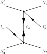
Figure 6: The Feynmann diagram corresponding to the lepton-nuclei scattering, $(N_{1},N_{2})+l_{\beta}^{-{}}\to(\text{neutrinos})\to(N_{1}^{\prime},N_{2}^{\prime})+l_{\alpha}^{+{}}$, with the $S$-matrix element given in Eq. (177).

Note that the propagation of internal neutrinos is shown by a broad line which means that it accounts for the interaction with background matter exactly.

Now we have to diagonalize the mass matrices $m_{\lambda\lambda^{\prime}}^{\mathrm{D}}$ and $m_{\lambda\lambda^{\prime}}^{\mathrm{L,R}}$ in Eq. (XII) by means of the matrix transformations (153), with the rectangular matrices $(U_{\lambda a})$ and $(V_{\lambda a})$ being nonunitary and independent. The amplitude of the process shown in Fig. 6 is nonzero if virtual neutrinos correspond to Majorana fields. That is why we introduce a new Majorana field $\psi_{a}=\Psi_{a}^{\mathrm{L}}+(\Psi_{a}^{\mathrm{L}})^{c}$ as in Sec. XI.2.

Let us rewrite the Lagrangian (XII) in terms of the Majorana fields $\psi_{a}$,

$$\mathcal{L}= \sum_{a}\bar{\psi}_{a}(\mathrm{i}\gamma^{\mu}\partial_{\mu}-m_{a})\psi_{a}-$$

$$-\sum_{ab}g_{ab}^{\mu}\overline{\psi_{a}^{\mathrm{L}}}\gamma_{\mu}\psi_{b}^{\mathrm{L}}-(\text{sources}),$$ (178)

where $(g_{ab}^{\mu})$ is the matrix of the effective potentials of the neutrino interaction with matter in the mass eigenstates basis which is defined in Eq. (25). In Eq. (XII) we do not present the expression for the sources in the explicit form since they are supposed to be localized in space.

With help of Eq. (153) the $T$-product of the neutrino-lepton currents in Eq. (177) takes the form,

$$\langle l_{\alpha}^{+{}}\left|T\{j_{\mu}(x)j_{\nu}(y)\}\right|l_{\beta}^{-{}}\rangle=\frac{e^{\mathrm{i}p_{\alpha}x-\mathrm{i}p_{\beta}y}}{2\mathcal{V}\sqrt{E_{\alpha}E_{\beta}}}\sum_{ab}U_{\alpha a}^{*{}}U_{\beta b}^{*{}}u^{\mathrm{T}}(-p_{\alpha})\left(\gamma_{\mu}^{\mathrm{L}}\right)^{\mathrm{T}}\langle 0|T\{\left[\bar{\psi}_{a}(x)\right]^{\mathrm{T}}\bar{\psi}_{b}(y)\}|0\rangle\gamma_{\nu}^{\mathrm{L}}u(p_{\beta}),$$ (179)

where $u(p_{\alpha,\beta})$ are the outgoing and incoming spinors with four momenta $p_{\alpha,\beta}=(E_{\alpha,\beta},\mathbf{p}_{\alpha,\beta})$ and $\mathcal{V}$ is the normalization volume. In Eq. (179) we use the representation of lepton states in the form of a plane wave from Ref. BerLifPit89 .

Since the mass of the nucleons is much bigger that the energies of leptons, we can suggest that they are at rest, i.e. we replace the nucleon currents

$$J_{\mu}(x)=\delta_{0\mu}\delta(\mathbf{x}-\mathbf{x}_{2}),\quad J_{\mu}(x)=\delta_{0\mu}\delta(\mathbf{y}-\mathbf{x}_{1}),$$ (180)

in Eq. (177).

The $T$-product of Majorana neutrino fields in Eq. (179) can be rewritten as (see, e.g., Ref. FukYan03p292 )

$$\langle 0|T\{\left[\bar{\psi}_{a}(x)\right]^{\mathrm{T}}\bar{\psi}_{b}(y)\}|0\rangle=-CS_{ab}(x-y),$$ (181)

where $C$ is the charge conjugation matrix and $S_{ab}(x-y)=\langle 0|T\{\psi_{a}(x)\bar{\psi}_{b}(y)\}|0\rangle$ is the usual Feynmann propagator corresponding to a Dirac particle.

To simplify the calculations we suggest that the matrix $(g_{ab}^{\mu})$ in Eq. (XII) is close to diagonal. Under this assumption the propagator in Eq. (181) has the diagonal form: $S_{ab}(x)=\delta_{ab}S_{a}(x)$. The explicit form of the function $S_{a}(x)$ is given in Appendix D. Moreover, as in Secs. III and V, we will study the situation of nonmoving and unpolarized matter, with matrix $(g_{ab}^{\mu})$ having only the zeroth component.

Using the results of Appendix D we can represent the $S$-matrix element in Eq. (177) as

$$S= 2\pi\delta(E_{\alpha}-E_{\beta})\frac{G_{\mathrm{F}}^{2}}{4\mathcal{V}\sqrt{E_{\alpha}E_{\beta}}}M_{\beta\alpha},$$

$$M_{\beta\alpha}= -\frac{e^{\mathrm{i}\mathbf{p}_{\beta}\mathbf{x}_{1}-\mathrm{i}\mathbf{p}_{\alpha}\mathbf{x}_{2}}}{2\pi L}$$

$$\times\sum_{a}m_{a}U_{\alpha a}^{*{}}U_{\beta a}^{*{}}\bar{u}(p_{\alpha})F_{a}u(p_{\beta}),$$ (182)

where

$$F_{a}= \frac{1}{2|g_{a}|p_{a}}\bigg{[}e^{\mathrm{i}k_{1}L}\left(\frac{g_{a}^{2}}{2}+|g_{a}|p_{a}-g_{a}k_{1}(\bm{\alpha}\mathbf{n})\right)$$

$$-e^{\mathrm{i}k_{2}L}\left(\frac{g_{a}^{2}}{2}-|g_{a}|p_{a}-g_{a}k_{2}(\bm{\alpha}\mathbf{n})\right)\bigg{]}$$

$$\times(1-\gamma^{5}),$$ (183)

and $k_{1,2}^{2}=(p_{a}\pm|g_{a}|/2)^{2}$, $p_{a}=\sqrt{E^{2}-m_{a}^{2}}$ is the neutrino “momentum”, $E=E_{\alpha}=E_{\beta}$ is the energy of leptons which is conserved since nucleons are supposed to be at rest.

Let us discuss the case of high energy leptons with $E_{\lambda}\gg m_{\lambda}$, where $m_{\lambda}$ is the lepton mass. In this case the biggest contribution to the matrix element of the total process arises from the channel in which the helicity of leptons changes from $-1/2$ to $1/2$. Thus the matrix element in Eq. (XII) takes the form,

$$M(l_{\beta}^{-{}}\to l_{\alpha}^{+{}})\approx -\frac{2e^{\mathrm{i}\mathbf{p}_{\beta}\mathbf{x}_{1}-\mathrm{i}\mathbf{p}_{\alpha}\mathbf{x}_{2}}}{\pi L}\sum_{a}Em_{a}U_{\alpha a}^{*{}}U_{\beta a}^{*{}}\langle F_{a}\rangle$$

$$\times e^{-\mathrm{i}\varphi/2}\sin\frac{\vartheta}{2},$$ (184)

where the spherical angles $\varphi$ and $\vartheta$ fix the direction of the outgoing lepton momentum with respect to the incoming lepton momentum, which, for simplicity, is chosen to be directed along the vector $\mathbf{L}$.

Using Eq. (XII) we can calculate the function $F_{a}$ in Eq. (XII) in the high energy leptons approximation,

$$\langle F_{a}\rangle= \bar{u}(p_{\alpha})F_{a}u(p_{\beta})$$ (185)

$$=\begin{cases}\displaystyle\left(1-\frac{|g_{a}|}{2p_{a}}\right)e^{\mathrm{i}(p_{a}-|g_{a}|/2)L},&\displaystyle\text{if $p_{a}>\frac{|g_{a}|}{2}$},\\ 0,&\displaystyle\text{if $p_{a}<\frac{|g_{a}|}{2}$}.\end{cases}$$

The details of the averaging over the lepton states in Eqs. (XII) and (185) can be found in Ref. Kob82 .

Finally the total cross section for the leptons scattering $(N_{1},N_{2})+l_{\beta}^{-{}}\to(\text{neutrinos})\to(N_{1}^{\prime},N_{2}^{\prime})+l_{\alpha}^{+{}}$ can be presented in the following form:

$$\sigma(l_{\beta}^{-{}}\to l_{\alpha}^{+{}})\sim \frac{G_{\mathrm{F}}^{4}E^{2}}{L^{2}}\sum_{ab}m_{a}m_{b}U_{\alpha a}^{*{}}U_{\beta a}^{*{}}U_{\alpha b}U_{\beta b}$$

$$\times\langle F_{a}\rangle\langle F_{b}^{*{}}\rangle\frac{v_{\alpha}}{v_{\beta}},$$ (186)

where $v_{\alpha,\beta}$ are the velocities of outgoing and incoming leptons. If we study the most general Lagrangian (XII), which contains both Dirac and Majorana mass matrices, Eqs. (185) and (XII) involve transitions between neutrinos and antineutrinos studied in Refs. Kob82 ; SchVal81v23 (see also Secs. VIII and XI).

Using Eqs. (185) and (XII) one can conclude that for light neutrinos with $m_{a}\ll E$ the matter contribution is negligible since $p_{a}\approx E-m_{a}^{2}/2E\gg|g_{a}|$. However the situation is completely different in the case of heavy neutrinos which are not excluded in some theoretical models Atr09 . If we study the neutrino propagation in the dense nuclear matter with $|g_{a}|\sim\text{eV}$, the “momentum” of such heavy neutrinos can be comparable with the effective potential of matter interaction at the appropriate choice of lepton energy. Nevertheless we can see in Eq. (185) that the contribution of such heavy mass eigenstates to neutrino-to-antineutrino transitions will be strongly suppressed by interaction with background matter. Note that such a behavior of the transition probability in presence of background matter is in agreement with the results of Ref. EspTan97 where oscillations between neutrinos and antineutrinos were studied in frames of the standard quantum mechanical approach.

In the derivation of the main results (185) and (XII) we neglected the contribution of the nondiagonal elements of the matrix $(g_{ab}^{\mu})$. One can expect that this contribution can be responsible for the enhancement of the probability of neutrino-to-antineutrino transitions as it can for neutrino flavor oscillation in matter (see Sec. III). If one takes into account these nondiagonal elements, the neutrino propagator in Eq. (181) also acquires nondiagonal entries. It is rather difficult to analyze this kind of “nondiagonal” propagators analytically. Thus, the approach for the description of neutrino oscillations based on the quantum field theory does not seem to be applicable for the situation of big nondiagonal elements of the matrix $(g_{ab}^{\mu})$.

XIII Conclusion

In conclusion we mention that in the present work we summarized our resent achievements in the theoretical description of neutrino oscillations in vacuum and external fields. Basically we studied three approaches: relativistic quantum mechanics approach (Secs. II-V, VIII, and IX), classical external sources method (Sec. XI), and quantum field theory treatment of neutrino oscillations (Sec. XII).

The formulation of the initial condition problem (2) for the system of flavor neutrinos is the main feature of the relativistic quantum mechanics method. Then one looks for wave functions of flavor neutrinos at subsequent moments of time. In vacuum the Cauchy problem for neutrino mass eigenstates (3) can be solved exactly [see Eq. (12)] giving us neutrino wave functions for arbitrary initial condition. When we study the time evolution of flavor neutrinos in presence of external fields within this formalism, we can reduce the dynamics of the system to a Schrödinger like equation [see, e.g., Eqs. (74) and (118)].

Note that, using this formalism, one solves not only the problem of the structure of the effective Hamiltonian but also we clearly point out what kind of space of wave functions this effective Hamiltonian acts in. In frames of the standard quantum mechanical approach GriPon69 ; LimMar88 one studies the evolution of a quantum mechanical neutrino “wave function” $\nu^{\mathrm{T}}=(\nu_{\alpha},\nu_{\beta},\dotsc)$, but the origin of the components of this wave function is disguised. Using the relativistic quantum mechanics method one immediately gets the answer to this questions. If we take the coefficients $a_{a}^{(\zeta)}$ of the decomposition of a four component neutrino wave function over the basis spinors [see, e.g., Eqs. (V) and (112)] and then make a certain transformation, like in Eqs. (73) and (117), of these coefficients, we arrive to the quantum mechanical neutrino “wave function”.

Note that in our approach the coefficients $a_{a}^{(\zeta)}$ are $c$-numbers rather than operators as in quantum field theory. It means that this method may be called as a classical field theory treatment of neutrino oscillations since we do not use second quantized neutrino wave functions.

Besides resolving the conceptual problem of neutrino oscillations, the relativistic quantum mechanics method can be applicable for the description of neutrino oscillations not only in vacuum (Sec. II), but also in background matter (Sec. III), spin flavor oscillations in an external magnetic field (Sec. IV), and in the combination of background matter and a magnetic field (Sec. V). Note that both Dirac and Majorana neutrinos can be treated within this formalism (see Secs. VIII and IX).

When we study the evolution of neutrinos in an external field, we use exact solutions of wave equations in this external field. That is why our treatment is valid for arbitrary strength of external fields. Moreover, the dynamics of mixed neutrinos is usually described in the mass eigenstates basis. In general case, external fields, like interaction with background matter or with an external electromagnetic field, are not diagonal in this basis [see Eqs. (25) and (45)], i.e. the neutrino mass eigenstates are not independent in presence of an external field [see, e.g., Eq. (V)]. Nevertheless in frames of the relativistic quantum mechanics method we can treat this kind of coupled mass eigenstates and receive results which are consistent with the standard quantum mechanical approach.

As it was mentioned above, the relativistic quantum mechanics method is a field theory counterpart of the usual quantum mechanical description of neutrino oscillation in a sense that it allows one to describe the evolution of mixed massive neutrinos from the first principles and thus it throws daylight upon some unclear issues of the quantum mechanical approach. However, trying to follow quantum mechanical approach as close as possible, we also adopted some of its weaknesses. For example, as in the quantum mechanical description, in frames of our method neutrino “wave functions” evolve in time rather than in space. It is, however, a contradiction with the majority of the experiments where one measures neutrino oscillations in space rather than in time.

Among other disadvantages of the present method we mention its limited applicability to description of neutrinos with small initial momentum in the case of nondiagonal external fields in the mass eigenstates basis. In this situation the ordinary differential equations for $a_{a}^{(\zeta)}(t)$ and $b_{a}^{(\zeta)}(t)$ evolution [see, e.g., Eq. (III)] start to entangle, making possible the transitions between “positive” and “negative” energy states. Thus, for example, instead of $4\times 4$ effective Schrödinger equation for spin flavor oscillations one gets $8\times 8$ differential equation, which is quite difficult for the analysis.

We should also mention the fact that to get the consistency with the quantum mechanical approach, one should consider rather broad initial wave packet [see Eq. (18)] which is rather difficult to implement in practice. In Sec II we also demonstrated, for the case of neutrino evolution in vacuum, that spatially limited initial wave packets do not reveal flavor oscillations since they propagate as massless particles.

As we mentioned above, the relativistic quantum mechanics approach predicts neutrino oscillations in time rather than in space as they are observed in experiments. To resolve this contradiction in Sec. XI we developed a new approach to the description of neutrino oscillations in vacuum which is based on the consideration of flavor neutrinos emitted by classical sources. Within this method one could study neutrino oscillations in space of both Dirac [Eqs. (151) and (152)] and Majorana [Eqs. (XI.2)] neutrinos. For the case of Majorana neutrinos we could also describe the transitions between neutrinos and antineutrinos [see Eq. (XI.2)]. This our result is also consistent with the previous studies Kob82 ; SchVal81v23 . In frames of this formalism we exactly take into account neutrino masses as well as examine what kind of neutrino sources could give us a stable oscillations picture (see also Appendix C).

However, the external classical source approach is not free from disadvantages. This method is based on the use of the retarded Green functions [Eqs. (135) and (XI.2)] in the neutrino mass eigenstates basis. Thus, if one tries to apply this formalism for the description of neutrino oscillations in an external field, which, as we mentioned above, is typically nondiagonal in the mass eigenstate basis, one encounters a problem to find a nondiagonal retarded Green function. It is quite difficult to calculate this kind of function analytically. Thus this approach is unlikely to be applicable to the description of neutrino oscillations in an external field, in contrast to the relativistic quantum mechanics method with gives satisfactory results in presence of external fields at least for ultrarelativistic neutrinos, unless we study a special case of an external field which is diagonal in the neutrino mass eigenstates basis.

We made an attempt to describe transitions between neutrinos and antineutrinos using the relativistic quantum mechanics method [Eq. (VIII)] and the external classical source approach [Eq. (XI.2)] and obtained the corresponding transition probability formulae which resemble the previously derived ones Kob82 ; SchVal81v23 . However, in case of Majorana neutrinos, particles are identical to their antiparticles. The concept of antiparticles is an inherent component of quantum field theory. Thus the approaches based on classical physics do not seem to be an appropriate tool for the description of oscillations between neutrinos and antineutrinos. That is why in Sec. XII we use the quantum field theory method to study particles and antiparticles in background matter in case of Majorana neutrinos. Note that the analogous method for the description of neutrino oscillations in vacuum was previously used in Refs. Kob82 ; GiuKimLeeLee93 ; Beu02 .

It should be noted that oscillations between neutrinos and antineutinos manifest in ($0\nu 2\beta$)-decay Bil10 . During this process two nucleons inside a nucleus exchange a virtual Majorana neutrino. That is why it is important to examine the influence of dense nuclear matter on the process of Majorana neutrinos propagation.

In our analysis we considered the situation when the interaction with matter is diagonal in the mass eigenstates basis since the case of a nondiagonal neutrino propagator is rather difficult to study analytically. This difficulty is analogous to that in the external classical source approach. Nevertheless we found that this type of matter interaction suppresses transitions between neutrinos and antineutrinos. Moreover, in case of hypothetical very heavy Majorana neutrinos the transition probability vanishes [see Eqs. (185) and (XII)]. It means that one cannot explore the presence of this kind of heavy neutrinos studying ($0\nu 2\beta$)-decay.

In Secs. VI, VII, and X we discussed several applications of the results obtained in frames of the relativistic quantum mechanics method to the studies of astrophysical neutrinos emitted during the core collapse of a supernova. First we studied spin flavor oscillations of Dirac (Sec. VI) and Majorana (Sec. X) neutrinos in an expanding envelope under the influence of the magnetic field of a supernova. It was found that for Dirac neutrinos the amplification of neutrino oscillations can be achieved in a moderate magnetic field [see Figs. 2(d)-4(d)]. On the contrary, in the Majorana neutrinos case, neutrino oscillations can be enhanced only in a strong magnetic field [see Fig. 5(b), (d) and (f)].

In Sec. VII another channel of oscillations of astrophysical neutrinos was considered. We studied the possibility of spin flavor oscillations between electron and additional quasi-degenerate in mass sterile neutrinos. We obtained that the correction (81) to the effective Hamiltonian (80), found in frames of the relativistic quantum mechanics method, results in the appearance of the new resonance in this oscillations channel.

Finally in Appendix A we present the general solution of the ordinary differential equations for the coefficients $a_{a}^{(\zeta)}$ which one encounters in the relativistic quantum mechanics method. In Appendix B we discuss the validity of the relativistic quantum mechanics approach to the description of neutrino spin flavor oscillations. In particular, we analyze various factors which influence oscillations between electron and sterile neutrinos with very small $\delta m^{2}$ (see also Sec. VII). In Appendix C we study how neutrino wave functions converge to the values corresponding to the stable oscillations picture in the external classical source approach (Sec. XI). In Appendix D we present the details of the calculation of the $S$-matrix element involving transitions between neutrinos and antineutrinos in frames of the quantum field theory description of neutrino oscillations (Sec. XII).

Summarizing we can say that a theoretical approach for the description of neutrino oscillations should satisfy the following requirements: the evolution equation governing the dynamics of mixed neutrinos should be derived from Lorentz invariant Lagrangian of the system and thus it should account for the relativistic invariance, at least implicitly; and such a method should be applicable in presence of various external fields. Among various theoretical approaches BerGuzNis10 ; Beu03 the relativistic quantum mechanics method is likely to be most appropriate formalism for the description of neutrino oscillations.

Appendix A Solution to the ordinary differential equations for the functions $a_{a}^{(\zeta)}$

In this Appendix we describe the formalism for the analysis of ordinary differential equations for the functions $a_{a}^{(\zeta)}$ which one encounters in Secs. III and IV.

Let us study the time evolution of the two component spinor $\mathbf{Z}^{\mathrm{T}}=(Z_{1},Z_{2})$ which is governed by the Schrödinger equation of the form,

$$\mathrm{i}\dot{\mathbf{Z}}=H\mathbf{Z},$$ (187)

where the Hamiltonian has the following form:

$$H=g\begin{pmatrix}0&e^{\mathrm{i}\omega t}\\ e^{-\mathrm{i}\omega t}&0\ \end{pmatrix}.$$ (188)

Here $g$ and $\omega$ are real parameters. Eq. (187) should be supplied with the initial condition $\mathbf{Z}(0)$. To find the solution of Eqs. (187) and (188) we introduce the new spinor $\mathbf{Z}^{\prime}$ by the relation, $\mathbf{Z}=\mathcal{U}\mathbf{Z}^{\prime}$, where the unitary matrix $\mathcal{U}$ reads

$$\mathcal{U}=\begin{pmatrix}e^{\mathrm{i}\omega t/2}&0\\ 0&e^{-\mathrm{i}\omega t/2}\ \end{pmatrix}.$$ (189)

Now Eq. (187) is rewritten in the following way:

$$\mathrm{i}\dot{\mathbf{Z}}^{\prime}=H^{\prime}\mathbf{Z}^{\prime},$$ (190)

with the new Hamiltonian $H^{\prime}$ which is obtained with help of Eqs. (187)-(189),

$$H^{\prime}=\mathcal{U}^{\dagger}H\mathcal{U}-\mathrm{i}\mathcal{U}^{\dagger}\dot{\mathcal{U}}=\begin{pmatrix}\omega/2&g\\ g&-\omega/2\ \end{pmatrix}.$$ (191)

Note that the initial condition for the spinor $\mathbf{Z}^{\prime}(0)$ is the same as for $\mathbf{Z}(0)$, $\mathbf{Z}^{\prime}(0)=\mathbf{Z}(0)$, due to the special form of the matrix $\mathcal{U}$ in Eq. (189).

Supposing that the Hamiltonian $H^{\prime}$ in Eqs. (190) and (191) does not depend on time we get the solution to Eq. (190) as

$$\mathbf{Z}^{\prime}(t)= \exp{(-\mathrm{i}H^{\prime}t)}\mathbf{Z}^{\prime}(0)$$

$$=\left(\cos\varOmega t-\mathrm{i}(\bm{\sigma}\mathbf{n})\sin\varOmega t\right)\mathbf{Z}^{\prime}(0),$$ (192)

where $\mathbf{n}=(g,0,\omega/2)/\varOmega$ is the unit vector and $\varOmega=\sqrt{g^{2}+(\omega/2)^{2}}$. Using Eqs. (189) and (A) we arrive to the expressions for the components of $\mathbf{Z}$ written in terms of the initial condition $\mathbf{Z}(0)$:

$$Z_{1}(t)= \left(\cos\varOmega t-\mathrm{i}\frac{\omega}{2\varOmega}\sin\varOmega t\right)e^{\mathrm{i}\omega t/2}Z_{1}(0)$$

$$-\mathrm{i}\frac{g}{\varOmega}\sin(\varOmega t)e^{\mathrm{i}\omega t/2}Z_{2}(0),$$

$$Z_{2}(t)= \left(\cos\varOmega t+\mathrm{i}\frac{\omega}{2\varOmega}\sin\varOmega t\right)e^{-\mathrm{i}\omega t/2}Z_{2}(0)$$

$$-\mathrm{i}\frac{g}{\varOmega}\sin(\varOmega t)e^{-\mathrm{i}\omega t/2}Z_{1}(0),$$ (193)

which can be directly applied for the analysis of ordinary differential equations from Secs. III and IV.

To get the solution of Eq. (III) we identify the components of the spinor $\mathbf{Z}$ with $a_{1,2}^{-{}}$ and the parameter $\omega$ with $\omega_{-{}}$ (see Sec. III). Finally we arrive to Eq. (III). We can also apply Eq. (A) to obtain the solution of Eq. (53). For this purpose one considers two cases:

• For $\mathbf{Z}^{\mathrm{T}}=(a_{1}^{+{}},a_{2}^{+{}})$, $g=-\mu B$, $\omega=\omega_{+{}}$ and $\varOmega=\Omega_{+{}}$;

• For $\mathbf{Z}^{\mathrm{T}}=(a_{1}^{-{}},a_{2}^{-{}})$, $g=\mu B$, $\omega=\omega_{-{}}$ and $\varOmega=\Omega_{-{}}$.

Using these formulae together with Eqs. (A) we readily arrive to Eqs. (IV)-(56). Note that the dynamics of the system (187) and (188) is analogous to the quantum mechanical description of neutrino spin flavor oscillation in a twisting magnetic field studied in Ref. Smi91 .

Appendix B Analysis of approximations made in the derivation of the effective Hamiltonian

In this Appendix we analyze the validity of the relativistic quantum mechanics approach for the description of neutrino spin flavor oscillations used in Sec. V. The correction to the effective Hamiltonian (81) is a rather small quantity. Therefore we should evaluate other factors which can also give the contributions, comparable with Eq. (81), to the effective Hamiltonian. In this section we analyze the contributions to the effective Hamiltonian from longitudinal magnetic field, matter polarization and possible corrections from the new interactions.

First we should remind that we use the relativistic quantum mechanics approach, with the external fields being independent of spatial coordinates. If external fields depend on the spatial coordinates, Dirac wave packets theory reveals various additional phenomena such as particles creation by the external field inhomogeneity ItzZub84p80 . For the approximation of the spatially constant external fields to be valid, the typical length scale of the external field variation $L_{\mathrm{ext}}$ should be much greater than the Compton length of a neutrino ItzZub84p80 : $L_{\mathrm{ext}}\gg\lambdabar_{C}=\hbar/m_{\nu}c$ DvoStu02 . For a neutrino with $m_{\nu}\sim 1\thinspace\text{eV}$ this condition reads $L_{\mathrm{ext}}\gg 10^{-5}\thinspace\text{cm}$, that is fulfilled for almost all realistic external fields.

A general remark on the “perturbative” approach used in Sec. V should be made. In the modified Eq. (III), which includes the interaction with the magnetic field, the terms containing $a_{a}^{\pm{}}$ and $a_{a}^{\mp{}}$ are coupled and the coupling terms are proportional to $g$ and $\mu B$ (V). As we demonstrate in Sec. II, mass eigenstates decouple in vacuum are their values depend on the initial condition only. While solving the modified Eq. (III), we could just take a term linear in $g$ and $\mu B$ (see, e.g., Eq. (IV) as well as Refs. Dvo06 ; DvoMaa07 ). However we take into account these terms exactly in the further analysis [see Eqs. (71) and (74)]. It is equivalent to the summation of all terms in the perturbation series.

While deriving the effective Hamiltonian (74) in Sec. V we supposed that magnetic field is transverse with respect to the neutrino motion. The effect of the longitudinal magnetic field on neutrino oscillations was studied in Ref. AkhKhl88 . It was found there that diagonal entries of the effective Hamiltonian receive additional small contributions $\mu_{a}B_{\parallel{}}(m_{a}/k)$. In order to neglect the longitudinal magnetic field contribution in comparison with our corrections (81), its strength should satisfy the condition,

$$\frac{B_{\parallel{}}}{B_{\perp{}}}\ll\frac{1}{16kB_{\perp{}}|\mu_{a}m_{a}-\mu_{b}m_{b}|}\left|\frac{m_{a}^{2}g_{a}^{3}}{\mathcal{M}_{a}^{2}}-\frac{m_{b}^{2}g_{b}^{3}}{\mathcal{M}_{b}^{2}}\right|,$$ (194)

where $B_{\perp{}}$ is the transverse component of the magnetic field.

A regular magnetic field of a supernova typically has both poloidal and toriodal components. Of course, an irregular turbulent magnetic field can be also present but its length scale appears to be quite small. A toroidal magnetic field can be $\sim 10^{16}\thinspace\text{G}$ and is concentrated near the equator of the star at the distance $\sim 10\thinspace\text{km}$ from the star center ArdBisMoi05 . Thus in our case a toroidal magnetic field is unlikely to significantly contribute to the dynamics of neutrino oscillations.

Let us evaluate the fraction of neutrinos for which the new correction (81) to the effective Hamiltonian gives bigger contribution to the resonance enhancement of oscillations compared to that of the longitudinal component of the poloidal magnetic field. Using Eq. (194) we find that these neutrinos should be emitted inside the solid angle near the equatorial plane with the spread $2\vartheta$, where $\vartheta\sim B_{\parallel{}}/B_{\perp{}}$. Assuming the radially symmetric neutrino emission we find that about 10% of the total neutrino flux is affected by the new resonance (95), i.e. the influence of the longitudinal magnetic field is negligible for oscillations of such particles.

The next important approximation made in the deviation of Eq. (74) was the assumption of negligible polarization of matter which can be not true if we study rather strong magnetic fields. The effect of matter polarization on neutrino oscillations was previously discussed in Refs. DvoStu02 ; Nun97 ; LobStu01 . Matter polarization produces the following contributions to the diagonal entries of the effective Hamiltonian DvoStu02 ; LobStu01 : $g_{a}(\bm{\lambda}_{f}\bm{\beta}_{\nu})$ (left polarized neutrinos) and $g_{a}(\bm{\lambda}_{f}\bm{\beta}_{\nu})(m_{a}/k)$ (right polarized neutrinos). Here $\bm{\beta}_{\nu}$ is the neutrino velocity and $\bm{\lambda}_{f}$ is the mean polarization vector of background fermions and we keep only the leading order in $m_{a}/k$.

First we estimate the contribution to the right polarized neutrinos effective potential. It is clear that one should take into account only the polarization of electrons since nucleons are much heavier. For the weakly degenerate electrons we should discuss the case of weak field limit (see Ref. Nun97 ), since $2eB/m_{e}^{2}\sim 10^{-8}\ll 1$, where $m_{e}$ is the electron’s mass and $B\sim 10^{7}\thinspace\text{G}$. Since the temperature inside the shock wave region can be about several MeV Sum05 the electrons are relativistic. Hence their mean polarization can be estimated as, $|\bm{\lambda}_{f}|\sim\mu_{\mathrm{B}}Bm_{e}/3T_{e}^{2}$, where $T_{e}$ is the temperature of electrons. Therefore we get that the new correction to the effective Hamiltonian (81) becomes bigger than the contribution of matter polarization to the effective potential of right polarized neutrinos at $T_{e}>4\thinspace\text{MeV}$.

To evaluate the contribution $g_{a}(\bm{\lambda}_{f}\bm{\beta}_{\nu})$ to the effective Hamiltonian, which corresponds to the left polarized neutrinos effective potential, we notice that the vector $\bm{\lambda}_{f}$ should be directed along the external magnetic field. For this term to be much less than the new correction to the effective Hamiltonian (81), the angle $\vartheta$, defined above, should be very small: $\vartheta\ll 10^{-8}$, for $T_{e}\sim 4\thinspace\text{MeV}$. It means that we can neglect the polarization effects only if neutrinos are emitted very close the equator of a star. We should, however, remind that this kind of matter polarization term contributes only to $(H_{QM})_{22}$ in Eq. (80) since only this entry corresponds to $\nu_{e}^{\mathrm{L}}$. Thus the presence of the term $g_{a}(\bm{\lambda}_{f}\bm{\beta}_{\nu})$ does not directly affect our results since we study $\nu_{e}^{\mathrm{R}}\leftrightarrow\nu_{s}^{\mathrm{L}}$ oscillations channel (see also Table 1).

The presence of big Dirac neutrino magnetic moments implies the existence of new interactions, beyond the standard model, which electromagnetically couple left and right polarized neutrinos. It is probable that these new interactions also contribute to the effective potential of the right polarized neutrino interaction with background matter. Despite this additional effective potential is likely to be small, one should evaluate it and compare with the correction (81).

The most generic $\mathrm{SU}(2)_{L}\times\mathrm{U}(1)_{Y}$ gauge invariant and remormalizable interaction which produces Dirac neutrino magnetic moment was discussed in Ref. Bel05 . It was found that neutrino magnetic moments arise from the effective Lagrangian involving the dimension $n=6$ operators $\mathcal{O}_{j}$,

$$\mathcal{L}_{\mathrm{eff}}=\sum_{j}\frac{C_{j}}{\Lambda^{2}}\mathcal{O}_{j}+\text{h.c.},$$ (195)

where $\Lambda\sim 1\thinspace\text{TeV}$ is a scale of the new physics and $C_{j}$ are the effective operator coupling constants. The sum in Eq. (195) spans all the operators of the given dimension.

One of the operators $\mathcal{O}_{j}$ also contributes to the effective potential of a right-handed neutrino in matter,

$$\mathcal{O}=\kappa\bar{L}\tau_{a}\tilde{\phi}\sigma^{\mu\nu}\nu_{\mathrm{R}}W_{\mu\nu}^{a},$$ (196)

where $\kappa$ is the coupling constant, $\tau_{a}$ are Pauli matrices, $L^{\mathrm{T}}=(\nu_{\mathrm{L}},e_{\mathrm{L}})$ is the $\mathrm{SU}(2)_{L}$ isodoublet, $\tilde{\phi}=\mathrm{i}\tau_{2}\phi^{*{}}$, with $\phi$ being a Higgs field, and $W_{\mu\nu}^{a}=\partial_{\mu}W_{\nu}^{a}-\partial_{\nu}W_{\mu}^{a}-\kappa\epsilon_{abc}W_{\mu}^{b}W_{\nu}^{c}$ is the $\mathrm{SU}(2)_{L}$ field strength tensor.

Assuming the spontaneous symmetry breaking at the electroweak scale, $\phi^{\mathrm{T}}\to(0,v/\sqrt{2})$, we can rewrite the Lagrangian in the form,

$$\mathcal{L}_{\mathrm{eff}}=\frac{C\kappa v}{\sqrt{2}}\bar{e}_{\mathrm{L}}\sigma^{\mu\nu}\nu_{\mathrm{R}}(W_{\mu\nu}^{1}-\mathrm{i}W_{\mu\nu}^{2})+\text{h.c.},$$ (197)

which implies that a process $e^{-{}}+\nu_{\mathrm{R}}\to e^{-{}}+\nu_{\mathrm{L}}$ should happen in background matter.

Using the results of Ref. Bel05 we can evaluate the contribution of the Lagrangian (197) to the effective Hamiltonian (80) as

$$\delta V_{\mathrm{R}}\sim V_{sm}\left(\frac{\mu_{\nu}}{\mu_{\mathrm{B}}}\right)^{2}\left(\frac{E_{\nu}}{m_{e}}\right)^{2}\frac{|\kappa|^{2}}{G_{\mathrm{F}}M_{W}^{2}},$$ (198)

where $V_{sm}\sim G_{\mathrm{F}}n_{e}$ is the standard model effective potential and $M_{W}$ is the $W$ boson mass. Taking $\mu_{\nu}\sim 10^{-12}\mu_{\mathrm{B}}$, $E_{\nu}\sim 100\thinspace\text{MeV}$ and $m_{\nu}\sim 1\thinspace\text{eV}$ (see Sec. VII) we can get that the ratio of the correction to the effective potential (198) and new correction (81) is $\sim 10^{-4}$. It means that the influence of new interactions, which generate neutrino magnetic moments, are not important for neutrino spin flavor oscillations.

Now let us estimate the influence of the diagonal magnetic moments $\mu_{a}$ on the dynamics of spin flavor oscillations. It was found in Ref. LycBli10 that to get the significant $\nu_{e}^{\mathrm{R}}$ luminosity $\sim 10^{50}\thinspace\text{erg/s}$ the diagonal magnetic moment should be $\mu_{\nu_{e}}=10^{-13}\thinspace\mu_{\mathrm{B}}$. Eq. (95) was obtained under the assumption $\mu_{\nu_{e}}\ll\mu$. In Eq. (97) we use $\mu=3\times 10^{-12}\thinspace\mu_{\mathrm{B}}$, i.e. the condition of the Eq. (95) validity is satisfied. In Fig. 7 we present the numerical solution of the Schrödinger equation (74).

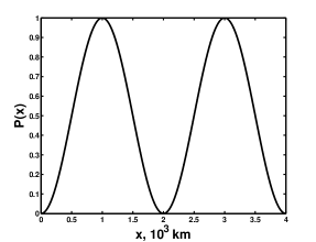
Figure 7: The numerical transition probability for neutrinos with $\mu=3\times 10^{-12}\thinspace\mu_{\mathrm{B}}$, $\mu_{\nu_{e}}=10^{-13}\thinspace\mu_{\mathrm{B}}$, $E=100\thinspace\mathrm{MeV}$, $m_{\nu_{e}}=1\thinspace\mathrm{eV}$ and $\delta m^{2}=5\times 10^{-17}\thinspace\mathrm{eV}^{2}$ moving in background matter with $\rho=10^{6}\thinspace\mathrm{g/cm}^{3}$ and interacting with the magnetic field $B=10^{7}\thinspace\mathrm{G}$. After Ref. Dvo10 .

We remind that our simplified model with $\mu_{\nu_{e}}=0$ gives the transition probability $P(x)=\sin^{2}(\mu Bx)$ if the resonance condition (95) is fulfilled. As one can see on Fig. 7 there is almost no difference in the dynamics of spin flavor oscillations in our simplified model and more realistic situation which involves non-zero diagonal magnetic moment of an electron neutrino.

Appendix C Evaluation of integrals

In this Appendix we calculate the integrals which one encounters while studying neutrino oscillations in the model with classical sources in Sec. XI. It is interesting to evaluate the inexactitude which is made when we approach to the limit $x_{m}\to\infty$ in Eq. (XI.1). Let us discuss two functions

$$F(r,t)= \int_{0}^{x_{m}}\mathrm{d}x\frac{J_{1}(mx)}{\sqrt{r^{2}+x^{2}}}e^{\mathrm{i}E\sqrt{r^{2}+x^{2}}}$$

$$=\int_{0}^{y_{m}}\mathrm{d}y\frac{J_{1}(\rho y)}{\sqrt{1+y^{2}}}e^{\mathrm{i}\mathcal{E}\sqrt{1+y^{2}}},$$ (199)

$$F_{0}(r)= \frac{1}{\rho}(e^{\mathrm{i}\mathcal{E}}-e^{\mathrm{i}P}).$$ (200)

These functions are proportional to $\mathcal{I}_{2}$ in Eqs. (XI.1) and (143) respectively. In Eqs. (C) and (200) we use dimensionless parameters $\rho=mr$, $\mathcal{E}=Er=\gamma\rho$, $\gamma=E/m$, $y_{m}=\sqrt{(t/r)^{2}-1}$ and $P=\sqrt{\mathcal{E}^{2}-\rho^{2}}$.

In case we study neutrinos, we get that $\mathcal{E}\gg\rho\gg 1$ in almost all realistic situations. For example, suppose we study a neutrino emitted in a supernova explosion is our Galaxy. The typical distance is $r\sim 10\thinspace\text{kpc}$. Taking $m\sim 1\thinspace\text{eV}$ and $E\sim 10\thinspace\text{MeV}$, we receive that $\mathcal{E}\sim 10^{35}$ and $\rho\sim 10^{28}$.

Basing on the analysis of Sec. XI.1 we can rewrite Eq. (C) as

$$F(r,t)= F_{0}(r)-\delta F,$$

$$\delta F= \int_{y_{m}}^{+\infty}\mathrm{d}y\frac{J_{1}(\rho y)}{\sqrt{1+y^{2}}}e^{\mathrm{i}\mathcal{E}\sqrt{1+y^{2}}}.$$ (201)

Using the fact that $\rho\gg 1$, $y_{m}\gg 1$ and the representation for the Bessel function,

$$J_{1}(z)\approx\sqrt{\frac{2}{\pi z}}\cos\left(z-\frac{3\pi}{4}\right)\quad\text{at}\quad z\to+\infty,$$ (202)

we obtain for the function $\delta F$ in Eq. (C) the following expression:

$$\delta F\approx -\frac{1}{\sqrt{2\pi\rho}}\big{\{}\mathrm{ci}([\gamma+1]\rho y_{m})+\mathrm{ci}([\gamma-1]\rho y_{m})$$

$$+\mathrm{i}[\mathrm{si}([\gamma+1]\rho y_{m})+\mathrm{si}([\gamma-1]\rho y_{m})]\big{\}},$$ (203)

where $\mathrm{ci}(z)$ and $\mathrm{si}(z)$ are cosine and sine integrals. Using the asymptotic expression,

$$|\mathrm{ci}(z)|\sim|\mathrm{si}(z)|\sim\frac{1}{z}\quad\text{at}\quad z\to+\infty,$$ (204)

we obtain that the function $\delta F$ approaches to zero as $1/(y_{m}\rho^{3/2})$ at great values of $y_{m}$ and $\rho$. Note that this result remains valid for a particle with an arbitrary $\gamma$ factor, i.e. rapid oscillations of the function $\delta F$ will attenuate even for slow particles. This analysis substantiates the approximations made in Sec. XI.1.

Finally let us illustrate the behavior of the functions $F(r,t)$ and $F_{0}(r)$. On Fig. 8 we present the absolute values of these functions versus $t$.

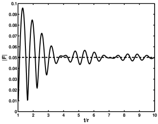
Figure 8: The absolute values of the functions $F(r,t)$ and $F_{0}(r)$ versus $t$. This figure is taken from Ref. Dvo09 .

This figure is plotted for $\rho=1$ and $\mathcal{E}=10$. The solid line is the absolute value of the function $F(r,t)$ and the dashed line of the function $F_{0}(r)$. As we mention in Sec. XI.1 the relaxation phenomena occur when $t\gtrsim r$. It can be also seen on Fig. 8. It is possible to notice that $|F(r,t)|\to|F_{0}(r)|$ at great values of $t$ as it is predicted in Sec. XI.1.

Appendix D Calculation of the $S$-matrix element

In this Appendix we present the detailed calculation of the $S$-matrix element in Sec. XII. Note that analogous calculation for the case of virtual neutrinos propagating in vacuum, i.e. when the matrix $(f_{\lambda\lambda^{\prime}}^{\mu})$ is absent in Eq. (XII), is presented in Ref. Kob82 .

Using Eqs. (179)-(181) as well as after the spatial integration and the elimination of the combinatorial factor we can cast Eq. (177) in the form,

$$S= \frac{G_{\mathrm{F}}^{2}}{\mathcal{V}\sqrt{E_{\alpha}E_{\beta}}}\int\mathrm{d}x_{0}\mathrm{d}y_{0}e^{\mathrm{i}\mathbf{p}_{\beta}\mathbf{x}_{1}-\mathrm{i}\mathbf{p}_{\alpha}\mathbf{x}_{2}}e^{\mathrm{i}E_{\alpha}x_{0}-\mathrm{i}E_{\beta}y_{0}}$$

$$\times\bar{u}(p_{\alpha})\gamma^{0}P_{\mathrm{R}}S_{a}(\mathbf{L},x_{0}-y_{0})P_{\mathrm{R}}\gamma^{0}u(p_{\beta}),$$ (205)

where we use the fact that $u^{\mathrm{T}}(-p_{\alpha})C=\bar{u}(p_{\alpha})$. The integration with respect to $x_{0}$ and $y_{0}$ can be performed with help of the new variables: $T=(x_{0}+y_{0})/2$ and $t=x_{0}-y_{0}$. After this integration one gets the energy conservation $\delta$-function in Eq. (XII).

The Fourier transform of the neutrino propagator $S_{a}(x)$ in Eq. (D) was found in Ref. PivStu05 and has the form,

$$S_{a}(k)=\frac{(k^{2}-m_{a}^{2}-g_{a}^{2}/4-\mathrm{i}\sigma_{\mu\nu}\gamma^{5}g_{a}^{\mu}k^{\nu})(\gamma^{\mu}k_{\mu}+m+\gamma_{\mu}\gamma^{5}g_{a}^{\mu}/2)}{(k^{2}-m^{2}-g_{a}^{2}/4)^{2}-(g_{a}k)^{2}+k^{2}g_{a}^{2}},$$ (206)

where $g_{a}^{\mu}\equiv g_{aa}^{\mu}$ are the diagonal elements of the matrix $(g_{ab}^{\mu})$ [see Eq. (25)].

In case of the nonmoving and unpolarized matter the momentum integration in Eq. (D) can be performed using the calculus of residues. Finally we arrive to the following result:

$$\int e^{\mathrm{i}\mathbf{k}\mathbf{L}}\frac{\mathrm{d}^{3}\mathbf{k}}{(2\pi)^{3}}\frac{p_{a}^{2}-g_{a}^{2}/4-\mathbf{k}^{2}-g_{a}(\bm{\alpha}\mathbf{k})}{(\mathbf{k}^{2}-k_{1}^{2})(\mathbf{k}^{2}-k_{2}^{2})}(1-\gamma^{5})\\ \approx-\frac{F_{a}}{4\pi L},$$ (207)

where $F_{a}$ is defined in Eq. (XII). In Eq. (207) we neglect several small terms since $k_{1,2}L\gg 1$.

It is convenient to perform momentum integration in Eq. (207) using cylindrical coordinates pointing $\mathbf{L}$ along the $z$-axis. Note that the integration over $k_{\phi}$ is trivial and gives $2\pi$ since the terms in the integrand [see also Eq. (206)] containing $k_{\phi}$ just vanish. The result of the integration over $\mathbf{k}$ can be presented in the form,

$$\int\frac{\mathrm{d}^{2}\mathbf{k}}{(2\pi)^{2}}\frac{F(k_{\rho},k_{z})}{(\mathbf{k}^{2}-k_{1}^{2})(\mathbf{k}^{2}-k_{2}^{2})}=J_{a}+J_{b}+J_{c},$$ (208)

where $\mathrm{d}^{2}\mathbf{k}=k_{\rho}\mathrm{d}k_{\rho}\mathrm{d}k_{z}$ and

$$J_{a}= \int_{0}^{k_{2}}\frac{k_{\rho}\mathrm{d}k_{\rho}}{(2\pi)^{2}}\int_{-\infty}^{+\infty}\mathrm{d}k_{z}\frac{F(k_{\rho},k_{z})}{(k_{z}^{2}-k_{z1}^{\prime 2})(k_{z}^{2}-k_{z2}^{\prime 2})},$$

$$J_{b}= \int_{k_{2}}^{k_{1}}\frac{k_{\rho}\mathrm{d}k_{\rho}}{(2\pi)^{2}}\int_{-\infty}^{+\infty}\mathrm{d}k_{z}\frac{F(k_{\rho},k_{z})}{(k_{z}^{2}-k_{z1}^{\prime 2})(k_{z}^{2}+k_{z2}^{\prime\prime 2})}$$

$$J_{c}= \int_{k_{1}}^{+\infty}\frac{k_{\rho}\mathrm{d}k_{\rho}}{(2\pi)^{2}}\int_{-\infty}^{+\infty}\mathrm{d}k_{z}\frac{F(k_{\rho},k_{z})}{(k_{z}^{2}+k_{z1}^{\prime\prime 2})(k_{z}^{2}+k_{z2}^{\prime\prime 2})}.$$ (209)

Here we use the notations $k_{z1,2}^{\prime}=\sqrt{k_{1,2}^{2}-k_{\rho}^{2}}$ and $k_{z1,2}^{\prime\prime}=\sqrt{k_{\rho}^{2}-k_{1,2}^{2}}$. The contours of the integration for each of the integrals in Eq. (D) are shown in Fig 9.

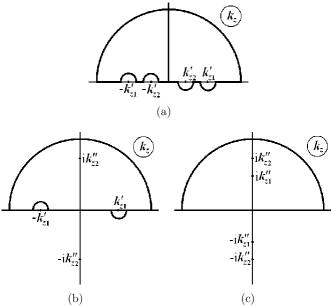
Figure 9: Integration contours for each of the integrals in Eq. (D). The panel (a) corresponds to $J_{a}$, (b) to $J_{b}$, and (c) to $J_{c}$.

References

- (1) K. Abe, et al. (Super-Kamiokande Collaboration), submitted to Phys. Rev. D, 1010.0118 [hep-ex]; B. Aharmim, et al. (SNO Collaboration), Phys. Rev. C 81, 055504 (2010), 0910.2984 [nucl-ex]; G. Bellini, et al. (Borexino Collaboration), Phys. Rev. D 82, 033006 (2010), 0808.2868 [astro-ph]; J. N. Abdurashitov, et al. (SAGE Collaboration), Phys. Rev. C 80, 015807 (2009), 0901.2200 [nucl-ex].
- (2) J. N. Bahcall and M. H. Pinsonneault, Phys. Rev. Lett. 92, 121301 (2004), astro-ph/0402114.
- (3) R. Wendell, et al. (Super-Kamiokande Collaboration), Phys. Rev. D 81, 092004 (2010), 1002.3471 [hep-ex]. B. Aharmim, et al. (SNO Collaboration), Phys. Rev. D 80, 012001 (2009), 0902.2776 [hep-ex].
- (4) R. Abbasi, et al. (IceCube Collaboration), Astropart. Phys. 34, 48 (2010), 1004.2357 [astro-ph.HE].
- (5) K. Hirata, et al. (Kamiokande II Collaboration), Phys. Rev. Lett. 58, 1490 (1987); R. M. Bionta, et al. (IMB Collaboration), Phys. Rev. Lett. 58, 1494 (1987); E. N. Alekseev et al., JETP Lett. 45, 589 (1987); V. L. Dadykin, et al., JETP Lett. 45, 593 (1987).
- (6) A. Gando, et al. (KamLAND Collaboration), Phys. Rev. D 83, 052002 (2011), 1009.4771 [hep-ex]; P. Adamson, et al. (MINOS Collaboration), Phys. Rev. D 82, 051102(R) (2010), 1006.0996 [hep-ex]; N. Agafonova, et al. (OPERA Collaboration), Phys. Lett. B 691, 138 (2010), 1006.1623 [hep-ex]; A. A. Aguilar-Arevalo, et al. (MiniBooNE Collaboration), Phys. Rev. Lett. 102, 101802 (2009), 0812.2243 [hep-ex].
- (7) Y. Kurimoto, et al. (SciBooNE Collaboration), Phys. Rev. D 81, 111102(R) (2010), 1005.0059 [hep-ex].
- (8) R. N. Mohapatra and A. Yu. Smirnov, Ann. Rev. Nucl. Part. Sci. 56, 569 (2006), hep-ph/0603118.
- (9) L. Wolfenstein, Phys. Rev. D 17, 2369 (1978); S. P. Mikheev and A. Yu. Smirnov, Sov. J. Nucl. Phys. 42, 913 (1985).
- (10) A. Cisneros, Astrophys. Space Sci. 10, 87 (1971); M. B. Voloshin, M. I. Vysotskiĭ, and L. B. Okun’, Sov. Phys. JETP 64, 446 (1986).
- (11) P. C. de Holanda and A. Yu. Smirnov, JCAP 0302, 001 (2003), hep-ph/0212270.
- (12) C. Biggio, M. Blennow, and E. Fernandez-Martinez, JHEP 0908, 090 (2009), 0907.0097 [hep-ph].
- (13) A. Yu. Ignatiev and G. C. Joshi, Phys. Rev. D 51, 2411 (1995), hep-ph/9407346; M. Dvornikov and A. Studenikin, Phys. Rev. D 69, 073001 (2004), hep-ph/0305206; M. Dvornikov and A. Studenikin, JETP 99, 254 (2004), hep-ph/0411085.
- (14) C. Giunti and A. Studenikin, Phys. Atom. Nucl. 72, 2089 (2009), 0812.3646 [hep-ph].
- (15) M. Fukugita and T. Yanagida, Physics of Neutrinos and Applications to Astrophysics (Springer, Berlin, 2003), pp. 461–479.
- (16) F. T. Avignone, III, S. R. Elliott, and J. Engel, Rev. Mod. Phys. 80, 481 (2008), 0708.1033 [nucl-ex].
- (17) S. M. Bilenky, Lect. Notes Phys. 817, 139 (2010), 1001.1946 [hep-ph].
- (18) J. Argyriades, et al. (NEMO Collaboration), Phys. Rev. C 80, 032501(R) (2009), 0810.0248 [hep-ex]; C. Arnaboldi, et al. (CUORICINO Collaboration), Phys. Rev. C 78, 035502 (2008), 0802.3439 [hep-ex].
- (19) S. M. Bilenky and B. Pontecorvo, Phys. Rept. 41, 225 (1978).
- (20) C.-S. Lim and W. J. Marciano, Phys. Rev. D 37, 1368 (1988).
- (21) B. Kayser, Phys. Rev. D 24, 110 (1981).
- (22) C. Guinti, JHEP 0211, 017 (2002), hep-ph/0205014.
- (23) A. D. Dolgov, et al., Eur. Phys. J. C 44, 431 (2005), hep-ph/0506203.
- (24) L. Stodolsky, Phys. Rev. D 58, 036006 (1998), hep-ph/9802387.
- (25) A. E. Bernardini, M. M. Guzzo, and C. C. Nishi, 1004.0734 [hep-ph].
- (26) I. Yu. Kobzarev, et al., Sov. J. Nucl. Phys. 35, 708 (1982).
- (27) C. Giunti, et al., Phys. Rev. D 48, 4310 (1993), hep-ph/9305276; W. Grimus and P. Stockinger, Phys. Rev. D 54, 3414 (1996), hep-ph/9603430.
- (28) A. Ioannisian and A. Pilaftsis, Phys. Rev. D 59, 053003 (1999), hep-ph/9809503.
- (29) D. V. Naumov and V. A. Naumov, J. Phys. G 37, 105014 (2010), 1008.0306 [hep-ph].
- (30) M. Blasone and G. Vitiello, Ann. Phys. 244, 283 (1995), hep-ph/9501263; Erratum ibid. 249, 363 (1996).
- (31) J. Wu, et al., Phys. Rev. D 82, 013006 (2010), 1005.3260 [hep-ph].
- (32) C. Anastopoulos and N. Savvidou, 1005.4307 [quant-ph].
- (33) M. Dvornikov, Phys. Lett B 610, 262 (2005), hep-ph/0411101; in Proceedings of the IPM School and Conference on Lepton and Hadron Physics, ed. by Y. Farzan, eConf C0605151 (2007), hep-ph/0609139.
- (34) M. Dvornikov, Eur. Phys. J. C 47, 437 (2006), hep-ph/0601156.
- (35) M. Dvornikov and J. Maalampi, Phys. Lett. B 657, 217 (2007), hep-ph/0701209.
- (36) M. Dvornikov, J. Phys. Conf. Ser. 110, 082005 (2008), 0708.2975 [hep-ph].
- (37) M. Dvornikov, J. Phys. G 35, 025003 (2008), 0708.2328 [hep-ph].
- (38) M. S. Dvornikov, Phys. Atom. Nucl. 72, 116 (2009), hep-ph/0610047.
- (39) M. Dvornikov and J. Maalampi, Phys. Rev. D 79, 113015 (2009), 0809.0963 [hep-ph].
- (40) M. Dvornikov, 1008.3115 [hep-ph].
- (41) A. E. Bernardini and S. De Leo, Phys. Rev. D 70, 053010 (2004), hep-ph/0411134; Eur. Phys. J. C 37, 471 (2004), hep-ph/0411153; Phys. Rev. D 71, 076008 (2005), hep-ph/0504239; C. C. Nishi, Phys. Rev. D 73, 053013 (2006), hep-ph/0506109.
- (42) K. Kiers and N. Weiss, Phys. Rev. D 57, 3091 (1998), hep-ph/9710289.
- (43) R. N. Mohapatra, New J. Phys. 6, 82 (2004), hep-ph/0411131.
- (44) I. Yu. Kobzarev, et al., Sov. J. Nucl. Phys. 32, 823 (1980).
- (45) J. Schechter and J. W. F. Valle, Phys. Rev. D 22, 2227 (1980).
- (46) N. N. Bogoliubov and D. D. Shirkov, Introduction to the Theory of Quantized Fields, (Wiley, New York, 1980), third ed., p. 607.
- (47) V. Gribov and B. Pontecorvo, Phys. Lett B 28, 493 (1969).
- (48) P. M. Morse and H. Feshbach, Methods of Theoretical Physics, (McGraw-Hill, New York, 1953), vol. 1, Chapter 7, pp. 854–857.
- (49) M. Dvornikov and A. Studenikin, JHEP 0209, 016 (2002), hep-ph/0202113.
- (50) A. E. Lobanov, and A. I. Studenikin, Phys. Lett. B 515, 94 (2001), hep-ph/0106101. A. Grigiriev, A. Lobanov, and A. Studenikin, Phys. Lett. B 535, 187 (2002), hep-ph/0202276.
- (51) A. Studenikin and A. Ternov, Phys. Lett B 608, 107 (2005), hep-ph/0412408. A. E. Lobanov, Phys. Lett B 619, 136 (2005), hep-ph/0506007.
- (52) M. Deniz, et al. (TEXONO Collaboration), Phys. Rev. D 82, 033004 (2010), 1006.1947 [hep-ph].
- (53) T. Kikuchi, H. Minakata, and S. Uchinami, JHEP 0903, 114 (2009), 0809.3312 [hep-ph].
- (54) A. G. Beda, et al., Phys. Atom. Nucl. 70, 1873 (2007), 0705.4576 [hep-ex].
- (55) E. Kh. Akhmedov and M. Yu. Khlopov, Sov. J. Nucl. Phys. 47, 689 (1988).
- (56) A. M. Egorov, A. E. Lobanov, and A. I. Studenikin, Phys. Lett. B 491, 137 (2000), hep-ph/9910476.
- (57) I. M. Ternov, V. G. Bagrov, and A. M. Khapaev, JETP 21, 613 (1965).
- (58) S. E. Woosley, A. Heger, and T. A. Weaver, Rev. Mod. Phys. 74, 1015 (2002).
- (59) G. G. Likhachev and A. I. Studenikin, JETP 81, 419 (1995).
- (60) S. Kawagoe, et al., J. Phys. Conf. Ser. 39, 294 (2006).
- (61) E. Kh. Akhmedov, A. Lanza, and D. W. Sciama, Phys. Rev. D 56, 6117 (1997), hep-ph/9702436.
- (62) D. Nötzold, Phys. Rev. D 38, 1658 (1988).
- (63) R. Barbieri and R. N. Mohapatra, Phys. Rev. Lett. 61, 27 (1988).
- (64) A. Ayala, J. C. D’Olivo, and M. Torres, Nucl. Phys. B 564, 204 (2000), hep-ph/9907398; A. V. Kuznetsov and N. V. Mikheev, JCAP 0711, 204 (2000), 0709.0110 [hep-ph].
- (65) A. V. Kuznetsov, N. V. Mikheev, and A. A. Okrugin, Int. J. Mod. Phys. A 24, 5977 (2009), 0907.2905 [hep-ph].
- (66) O. Lychkovskiy and S. Blinnikov, Phys. Atom. Nucl. 73, 614 (2010), 0905.3658 [hep-ph].
- (67) R. Tòmas, et al., JCAP 0409, 015 (2004), astro-ph/0407132.
- (68) P. Keränen, et al., Phys. Lett. B 574, 162 (2003), hep-ph/0307041; ibid. 597, 374 (2004), hep-ph/0401082.
- (69) V. A. Kutvitskiĭ, V. B. Semikoz, and D. D. Sokoloff, Astron. Rep. 53, 166 (2009), 0809.3172 [astro-ph]; C. R. Das, J. Pulido, and M. Picariello, Phys. Rev. D 79, 073010 (2010), 0902.1310 [hep-ph].
- (70) J. Maalampi and J. Riittinen, Phys. Rev. D 81, 037301 (2010), 0912.4628 [hep-ph].
- (71) A. Esmaili, Phys. Rev. D 81, 013006 (2010), 0909.5410 [hep-ph].
- (72) G. G. Raffelt, Phys. Rev. Lett. 64, 2856 (1990).
- (73) S. Akiyama, et al., Astrophys. J 584, 954 (2003), astro-ph/0208128.
- (74) See pp. 292–296 in Ref. FukYan03p461 .
- (75) K. M. Case, Phys. Rev. 107, 307 (1957).
- (76) V. B. Berestetskiĭ, E. M. Lifschitz, and L. P. Pitaevskiĭ, Quantum Electrodynamics (Moscow, Nauka, 1989), pp. 108–112.
- (77) See pp. 137–141 in Ref. BerLifPit89 .
- (78) J. Schechter and J. W. F. Valle, Phys. Rev. D 24, 1883 (1981).
- (79) D. Giulini, et al., Decoherence and the Appearence of a Classical World in Quantum Theory (Springer, Berlin, 1996).
- (80) See pp. 477–478 in Ref. FukYan03p461 .
- (81) S. Pastor, Master’s Thesis (University of Valencia, 1996).
- (82) S. Ando and K. Sato, Phys. Rev. D 68, 023003 (2003), hep-ph/0305052.
- (83) S. Ando and K. Sato, JCAP 0310, 001 (2003), hep-ph/0309060.
- (84) M. Kachelrieß, et al., Phys. Rev. D 65, 073016 (2002), hep-ph/0108100.
- (85) R. E. Shrock, Phys. Lett. B 96, 159 (1980).
- (86) C. Itzykson and J.-B. Zuber, Quantum Field Theory (McGraw-Hill, Ney York, 1980), pp. 692–969.
- (87) L. B. Okun’, Leptons and Quarks (Nauka, Moscow, 1990), 2nd ed., pp. 36–41.
- (88) See pp. 140–141 and 602–607 in Ref. BogShi80 .
- (89) Z.-Z. Xing, Phys. Lett. B 660, 515 (2008), 0709.2220 [hep-ph].
- (90) E. Kh. Akhmedov and A. Yu. Smirnov, Phys. Atom. Nucl. 72, 1363 (2009), 0905.1903 [hep-ph].
- (91) B. Pontecorvo, JETP 7, 172 (1958); for the contemporary description see pp. 286–287 in Ref. FukYan03p461 .
- (92) J. Schechter and J. W. F. Valle, Phys. Rev. D 23, 1666 (1981); A. de Gouvêa, B. Kayser, and R. N. Mohapatra, Phys. Rev. D 67, 053004 (2003), hep-ph/0211394.
- (93) S. Esposito and N. Tancredi, Mod. Phys. Lett. A 12, 1829 (1997), hep-ph/9705351.
- (94) M. Beuthe, Phys. Rev. D 66, 013003 (2002), hep-ph/0202068.
- (95) A. Atre, et al., JHEP 0905, 030 (2009), 0901.3589 [hep-ph].
- (96) M. Beuthe, Phys. Rep. 375, 105 (2003), hep-ph/0109119.
- (97) A. Yu. Smirnov, Phys. Lett B 260, 161 (1991); E. Kh. Akhmedov, P. I. Krastev, and A. Yu. Smirnov, Z. Phys. C 48, 701 (1991).
- (98) See pp. 60–63 in Ref. ItzZub84p385 .
- (99) N. V. Ardeljan, S. G. Bisnovatyi-Kogan, and S. G. Moiseenko, MNRAS 359, 333 (2005), astro-ph/0410234.
- (100) H. Nunokawa, et al., Nucl. Phys. B 501, 17 (1997), hep-ph/9701420.
- (101) K. Sumiyoshi, et al., Astrophys. J. 629, 922 (2005), astro-ph/0506620.
- (102) N. F. Bell, et al., Phys. Rev. Lett. 95, 151802 (2005), hep-ph/0504134.
- (103) I. Pivovarov and A. Studenikin, PoS HEP2005, 191 (2006), hep-ph/0512031.