Attempt-time Monte Carlo: an alternative for simulation of stochastic jump processes with time-dependent transition rates

Abstract

We present a new method for simulating Markovian jump processes with time-dependent transitions rates, which avoids the transformation of random numbers by inverting time integrals over the rates. It relies on constructing a sequence of random time points from a homogeneous Poisson process, where the system under investigation attempts to change its state with certain probabilities. With respect to the underlying master equation the method corresponds to an exact formal solution in terms of a Dyson series. Different algorithms can be derived from the method and their power is demonstrated for a set of interacting two-level systems that are periodically driven by an external field.

I Introduction

Stochastic jump processes with time-dependent transition rates are of general importance for many applications in physics and chemistry, in particular for describing the kinetics of chemical reactions Gibson/Bruck:2000 ; Anderson:2007 ; Astumian:2007 and the non-equilibrium dynamics of driven systems in statistical mechanics Crooks:1999 ; Seifert:2005 ; Esposito/VandenBroeck:2010 . With respect to applications in interdisciplinary fields they play an important role in connection with queuing theories.

In general a system with $N$ states is considered that at random time instants performs transitions from one state to another. In case of a Markovian jump dynamics the probability for the system to change its state in the time interval $[t,t+\Delta t[$ is independent of the history and given by $w_{ij}(t)\Delta t+o(\Delta t)$, where $j$ and $i\neq j$ are the initial and target state, respectively, and $w_{ij}(t)$ the corresponding transition rate at time $t$ ($w_{jj}(t)=0$). This implies that, if the systems is in the state $j$ at time $t_{0}$, it will stay in this state until a time $t>t_{0}$ with probability $\phi_{j}(t,t_{0})=\exp[-\int_{t_{0}}^{t}d\tau\,w_{j}^{\rm tot}(\tau)]$, where $w_{j}^{\rm tot}(\tau)=\sum_{i}w_{ij}(\tau)$ is the total escape rate from state $j$ at time $\tau$. The probability to perform a transition to the target state $i$ in the time interval $[t,t+dt[$ then is $w_{ij}(t)\phi_{j}(t,t_{0})dt$, i. e.

$$\psi_{ij}(t,t_{0})=w_{ij}(t)\exp\left[-\int_{t_{0}}^{t}d\tau\,w_{j}^{\rm tot}(\tau)\right]$$ (1)

is the probability density for the first transition to state $i$ to occur at time $t$ after the system was in state $j$ at time $t_{0}$. Any algorithm that evolves the system according to Eq. (1) generates stochastic trajectories with the correct path probabilities.

The first algorithm of this kind was developed by Gillespie Gillespie:1978 in generalization of the continuous-time Monte-Carlo algorithm introduced by Bortz et al. Bortz/etal:1975 for time-independent rates. We call it the reaction time algorithm (RTA) in the following. The RTA consists of drawing a random time $t$ from the first transition time probability density $\psi_{j}^{\rm tot}(t,t_{0})=\sum_{i}\psi_{ij}(t,t_{0})=w_{j}^{\rm tot}\phi_{j}(t,t_{0})=-\partial_{t}\phi_{j}(t,t_{0})$ to any other state $i\neq j$, and a subsequent random selection of the target state $i$ with probability $w_{ij}(t)/w_{j}^{\rm tot}(t)$. In practice these two steps can be performed by generating two uncorrelated and uniformly distributed random numbers $r_{1}$, $r_{2}$ in the unit interval $[0,1[$ with some random number generator, where the first is used to specify the transition time $t$ via

$$W_{j}(t,t_{0})=\int_{t_{0}}^{t}d\tau w_{j}^{\rm tot}(\tau)=-\log(1-r_{1})$$ (2)

and the second is used to select the target state $i$ by requiring

$$\sum_{k=1}^{i-1}\frac{w_{kj}(t)}{w_{j}^{\rm tot}(t)}\leq r_{2}<\sum_{k=1}^{i}\frac{w_{kj}(t)}{w_{j}^{\rm tot}(t)}$$ (3)

Both steps, however, lead to some unpleasant problems in the practical realization.

The first step according to Eq. (2) requires the calculation of $W_{j}(t,t_{0})$ and the determination of its inverse $\tilde{W}_{j}(.,t_{0})$ with respect to $t$ in order to obtain the transition time $t=\tilde{W}_{j}(-\log(1-r_{1}),t_{0})$. While this is always possible, since $w_{j}^{\rm tot}>0$ and accordingly $W_{j}(t,t_{0})$ is a monotonously increasing function of $t$, it can be CPU time consuming in case $W_{j}(t,t_{0})$ cannot be explicitly given in an analytical form and one needs to implement a root finding procedure.

The second step according to Eq. (3) can be cumbersome in case there are many states ($N$ large) and a systematic grouping of the $w_{ij}(t)$ to only a few classes is not possible. This situation in particular applies to many-particle systems, where $N$ typically grows exponentially with the number of particles, and the interactions (or a coupling to spatially inhomogeneous time-dependent external fields) can lead to a large number of different transitions rates. Moreover, even for systems with simple interactions (as, for example, Ising spin systems), where a grouping is in principle possible, the subdivision of the unit interval underlying Eq. (3) cannot be strongly simplified for time-dependent rates.

A way to circumvent Eq. (3) is the use of the First Reaction Time Algorithm (FRTA) for time dependent rates Jansen:1995 , or modifications of it Anderson:2007 . In the FRTA one draws random first transition times $t_{k}$ from the probability densities $\psi_{kj}(t_{k},t_{0})=w_{kj}(t_{k})\exp[-\int_{t_{0}}^{t_{k}}d\tau\,w_{kj}(\tau)]$ for the individual transitions to each of the target states $k$ and performs the transition $i$ with the smallest $t_{i}=\min_{k}\{t_{k}\}$ at time $t_{i}$. This is statistically equivalent to the RTA, since for the given initial state $j$, the possible transitions to all target states are independent of each other. In short-range interacting systems, in particular, many of the random times $t_{k}$ can be kept for determining the next transition following $i$. In fact, all transitions from the new state $i$ to target states $k$ can be kept for which $w_{ki}(\tau)=w_{kj}(\tau)$ for $\tau>t$ (see Ref. Einax/Maass:2009 for details). However, the random times $t_{k}$ need to be drawn from $\psi_{kj}(t_{k},t_{0})$ and this unfortunately involves the same problems as discussed above in connection with Eq. (2).

II Algorithms

We now present a new “attempt time algorithm” (ATA) that allows one to avoid the problems associated with the generation of the transition time in Eq. (2). Starting with the system in state $j$ at time $t_{0}$ as before, one first considers a large time interval $T$ and determines a number $\mu_{j}^{\rm tot}$ satisfying

$$\mu_{j}^{\rm tot}\geq\max_{t_{0}\leq\tau\leq t_{0}+T}\{w_{j}^{\rm tot}(\tau)\}\,\,.$$ (4)

In general this can by done easily, since $w_{j}^{\rm tot}(\tau)$ is a known function. In particular for bounded transition rates it poses no difficulty, as, for example, in the case of Glauber rates or a periodic external driving, where $T$ could be chosen as the time period. If an unlimited growth of $w_{j}^{\rm tot}$ with time were present (an unphysical situation for long times), $T$ can be chosen self-consistently by requiring that the time $t$ for the next transition to another state $i\neq j$ (see below) must be smaller than $t_{0}+T$.

Next an attempt time interval $\Delta t_{1}$ is drawn from the exponential density $F_{j}(\Delta t_{1})=\mu_{j}^{\rm tot}\exp(-\mu_{j}^{\rm tot}\Delta t_{1})$ and the resulting attempt transition time $t_{1}=t_{0}+\Delta t_{1}$ is rejected with probability $p_{j}^{\rm rej}(t_{1})=1-w_{j}^{\rm tot}(t_{1})/\mu_{j}^{\rm tot}$. If it is rejected, a further attempt time interval $\Delta t_{2}$ is drawn from $F_{j}(\Delta t_{2})$, corresponding to an attempt transition time $t_{2}=t_{1}+\Delta t_{2}$, and so on until an attempt time $t<t_{0}+T$ is eventually accepted. Then a transition to a target state $i$ is performed at time $t$ with probability $w_{ij}(t)/w_{j}^{\rm tot}(t)$, using the target state selection of Eq. (3).

In order to show that this method yields the correct first transition probability density $\psi_{ij}(t,t_{0})$ from Eq. (1), let us first consider a sequence, where exactly $n\geq 0$ attempts at some times $t_{1}<\ldots<t_{n}$ are rejected and then the $(n+1)$th attempt leads to a transition to the target state $i$ in the time interval $[t,t+dt[$. The corresponding probability density $\psi_{ij}^{(n)}(t,t_{0})$ is given by

$$\psi_{ij}^{(n)} (t,t_{0})=\int_{t_{0}}^{t}dt_{n}\int_{t_{0}}^{t_{n-1}}dt_{n-1}\ldots\int_{t_{0}}^{t_{2}}dt_{1}\frac{w_{ij}(t)}{w_{j}^{\rm tot}(t)}$$

$$\times\left[1-p_{j}^{\rm rej}(t)\right]F_{j}(t-t_{n})\prod_{m=1}^{n}p_{j}^{\rm rej}(t_{m})F_{j}(t_{m}-t_{m-1})$$ (5)

$$=\frac{w_{ij}(t)e^{-\mu_{j}^{\rm tot}(t-t_{0})}}{n!}\left[\int_{t_{0}}^{t}d\tau\,\mu_{j}^{\rm tot}p_{j}^{{\rm rej}}(\tau)\right]^{n}$$

$$=\frac{w_{ij}(t)e^{-\mu_{j}^{\rm tot}(t-t_{0})}}{n!}\left[\mu_{j}^{\rm tot}(t-t_{0})-\int_{t_{0}}^{t}d\tau\,w_{j}^{\rm tot}(\tau)\right]^{n}.$$

Summing over all possible $n$ hence yields

$$\psi_{j}(t,t_{0})=\sum_{n=0}^{\infty}\psi_{ij}^{(n)}(t,t_{0})=w_{ij}(t)\exp\left[-\int_{t_{0}}^{t}d\tau\,w_{j}^{\rm tot}(\tau)\right]$$ (6)

from Eq. (1).

It is clear that for avoiding the root finding of Eq. (2) by use of the ATA, one has to pay the price for introducing rejections. If the typical number of rejections can be kept small and an explicit analytical expression for $t$ cannot be derived from Eq. (2), the ATA should become favorable in comparison to the RTA. Moreover, the ATA can be implemented in a software routine independent of the special form of the $w_{ij}(\tau)$ for applicants who are not interested to invest special thoughts on how to solve Eq. (2).

One may object that the ATA still entails the problem connected with the cumbersome target state selection by Eq. (3). However, as the RTA has the first reaction variant FRTA, the ATA has a first attempt variant. In this first attempt time algorithm (FATA) one first determines, instead of $\mu_{j}^{\rm tot}$ from Eq. (4), upper bounds for the individual transitions to all target states $k\neq j$ ($\mu_{jj}=0$),

$$\mu_{kj}\geq\max_{t_{0}\leq\tau\leq t_{0}+T}\{w_{kj}(\tau)\}\,\,.$$ (7)

Thereon random time intervals $\Delta t_{k}$ are drawn from $F_{kj}(\Delta t_{k})=\mu_{kj}\exp(-\mu_{kj}\Delta t_{k})$, yielding corresponding attempt transition times $t_{k}^{(1)}=t_{0}+\Delta t_{k}$. The transition to the target state $k^{\prime}$ with the minimal $t_{k^{\prime}}^{(1)}=\min_{k}\{t_{k}^{(1)}\}=t_{1}$ is attempted and rejected with probability $p_{k^{\prime}k}^{\rm rej}(t_{k^{\prime}}^{(1)})=1-w_{k^{\prime}k}(t_{k^{\prime}}^{(1)})/\mu_{k^{\prime}k}$. If it is rejected, a further time interval $\Delta t_{k^{\prime}}^{(2)}$ is drawn from $F_{k^{\prime}j}(\Delta t_{k^{\prime}}^{(2)})$, yielding $t_{k^{\prime}}^{(2)}=t_{k^{\prime}}^{(1)}+\Delta t_{k^{\prime}}^{(2)}$, while the other attempt transition times are kept, $t_{k}^{(2)}=t_{k}^{(1)}$ for $k\neq k^{\prime}$ (it is not necessary to draw new time intervals for these target states due to the absence of memory in the Poisson process). The target state $k^{\prime\prime}$ with the new minimal $t_{k^{\prime\prime}}^{(2)}=\min_{k}\{t_{k}^{(2)}\}=t_{2}$ is then attempted and so on until eventually a transition to a target state $i$ is accepted at a time $t<t_{0}+T$. The determination of the minimal times can be done effectively by keeping an ordered stack of the attempt times. Furthermore, as in the FRTA, one can, after a successful transition to a target state $i$ at time $t$, keep the (last updated) attempt times $t_{k}$ for all target states that are not affected by this transition (i. e. for which $w_{ki}(\tau)=w_{kj}(\tau)$ for $\tau\geq t$). Overall one can view the procedure implied by the FATA as that each state $k$ has a next attempt time $t_{k}$ (with $t_{j}=\infty$ if the system is in state $j$) and that the next attempt is made to the target state with the minimal $t_{k}$. After each attempt, updates of some of the $t_{k}$ are made as described above in dependence of whether the attempt was rejected or accepted.

In order to prove that the FATA gives the $\psi_{j}(t,t_{0})$ from Eq. (1), we show that the probability densities $\chi_{ij}(t,t_{n})=[w_{ij}(t)/w_{j}^{\rm tot}(t)](1-p_{j}^{\rm rej}(t))F_{j}(t-t_{n})=w_{ij}(t)\exp[-\mu_{j}^{\rm tot}(t-t_{n})]$ and $\eta_{j}(t_{m},t_{m-1})=p_{j}^{\rm rej}(t_{m})F_{j}(t_{m}-t_{m-1})=[\mu_{j}^{\rm tot}-w_{j}^{\rm tot}]\exp[-\mu_{j}^{\rm tot}(t_{m}-t_{m-1})]$ appearing in Eq. (II) are generated, if we set $\mu_{j}^{\rm tot}=\sum_{k}\mu_{kj}$ (note that Eq. (4) is automatically satisfied by this choice). These probability densities have the following meaning: $\chi_{ij}(t,t_{n})dt$ is the probability that, if the system is in state $j$ at time $t_{n}$, the next attempt to a target state occurs in the time interval $[t,t+dt[$, the attempt is accepted, and it changes the state from $j$ to $i$; $\eta_{j}(t_{m},t_{m-1})dt_{m}$ is the probability that, after the attempt time $t_{m}$, the next attempt occurs in $[t_{m},t_{m}+dt_{m}[$ with $t_{m}>t_{m-1}$ and is rejected.

In the FATA the probability $\kappa_{lj}(t_{m},t_{m-1})dt_{m}$ that, when starting at time $t_{m-1}$, the next attempt is occurring in $[t_{m},t_{m}+dt_{m}[$ to a target state $l$ is given by

$$\kappa_{lj}(t_{m},t_{m-1}) =\mu_{lj}\exp[-\mu_{lj}(t_{m}-t_{m-1})]$$

$$\hskip 8.5359pt\times\prod_{k\neq l}\int_{t_{m}-t_{m-1}}^{\infty}d\tau\,\mu_{kj}\exp(-\mu_{kj}\tau)$$

$$=\mu_{lj}\exp[-\mu_{j}^{\rm tot}(t_{m}-t_{m-1})]\,\,.$$ (8)

The product ensures that $t_{m}$ is the minimal time (the lower bound in the integral can be set equal to $(t_{m}-t_{m-1})$ for all $k\neq l$ due to the absence of memory in the Poisson process). The probability that this attempted transition is rejected is $p_{lj}^{\rm rej}(t_{m})=1-w_{lj}(t_{m})/\mu_{lj}$ and accordingly, by summing over all target states $l$, we obtain

$$\eta_{j}(t_{m},t_{m-1}) =\sum_{l}p_{lj}^{\rm rej}(t_{m})\mu_{lj}\exp[-\mu_{j}^{\rm tot})(t_{m}-t_{m-1})]$$

$$=[\mu_{j}^{\rm tot}-w_{j}^{\rm tot}(t_{m})]\exp[-\mu_{j}^{\rm tot}(t_{m}-t_{m-1})]$$ (9)

in agreement with the expression appearing in Eq. (II). Furthermore, when starting from time $t_{n}$, the probability density $\chi_{ij}(t,t_{n})$ referring to the joint probability that the next attempted transition occurs in $[t,t+dt[$ to state $i$ and is accepted is given by

$$\chi_{ij}(t,t_{n})=\frac{w_{ij}(t)}{\mu_{ij}}\kappa_{ij}(t,t_{n})=w_{ij}(t)\exp[-\mu_{j}^{\rm tot}(t-t_{n})]\,\,.$$ (10)

Hence one recovers the decomposition in Eq. (II) with $\mu_{j}^{\rm tot}=\sum_{k}\mu_{kj}$.

Before discussing an example, it is instructive to see how the ATA (and RTA) can be associated with a solution of the underlying master equation

$$\frac{\partial}{\partial t}\,\mathbb{G}(t,t^{\prime})=-\mathbb{M}(t)\,\mathbb{G}(t,t^{\prime})\,\,,\qquad\mathbb{G}(t^{\prime},t^{\prime})=\mathbb{I}$$ (11)

where $\mathbb{G}(t,t^{\prime})$ is the matrix of transition probabilities $G_{ij}(t,t^{\prime})$ for the system to be in state $i$ at time $t$ if it was in state $j$ at time $t^{\prime}\leq t$, and $\mathbb{M}(t)$ is the transition rate matrix with elements $M_{ij}(t)=-w_{ij}(t)$ for $i\neq j$ and $M_{jj}(t)=-\sum_{i\neq j}M_{ij}(t)=w_{j}^{\rm tot}(t)$. Let us decompose $\mathbb{M}(t)$ as $\mathbb{M}(t)=\mathbb{D}+\mathbb{A}(t)$, where $\mathbb{D}=\mathrm{diag}\left\{\mu_{1}^{\rm tot},\ldots,\mu_{N}^{\rm tot}\right\}$. If $\mathbb{A}(t)$ were missing, the solution of the master equation (11) would be $\mathbb{G}_{0}(t,t^{\prime})=\mathrm{diag}\left\{\exp(-\mu_{1}^{\rm tot}(t-t^{\prime}),\ldots,\exp(-\mu_{N}^{\rm tot}(t-t^{\prime})\right\}$. Hence, when introducing $\tilde{\mathbb{A}}(t,t^{\prime})=\mathbb{G}_{0}^{-1}(t,t^{\prime})\mathbb{A}(t)\mathbb{G}_{0}(t,t^{\prime})=\mathbb{G}_{0}(t^{\prime},t)\mathbb{A}(t)\mathbb{G}_{0}(t,t^{\prime})$ in the “interaction picture”, the solution of the master equation can be written as

$$\mathbb{G}(t,t^{\prime}) =\mathbb{G}_{0}(t,t^{\prime})\left[\mathbb{I}+\int_{t^{\prime}}^{t}dt_{1}\tilde{\mathbb{A}}(t_{1},t^{\prime})\right.$$

$$\hskip 8.5359pt+\left.\int_{t^{\prime}}^{t}dt_{2}\int_{t^{\prime}}^{t_{2}}dt_{1}\tilde{\mathbb{A}}(t_{2},t^{\prime})\tilde{\mathbb{A}}(t_{1},t^{\prime})+\ldots\right]$$ (12)

Inserting $\mathbb{I}=\mathbb{D}^{-1}\mathbb{D}$ after each matrix $\tilde{\mathbb{A}}$, one arrives at

$$\mathbb{G}(t,t^{\prime})=\mathbb{G}_{0}(t,t^{\prime})+\int_{t^{\prime}}^{t}dt_{1}\mathbb{G}_{0}(t,t_{1})\mathbb{B}(t_{1})F_{0}(t_{1},t^{\prime})$$

$${}+\int_{t^{\prime}}^{t}dt_{2}\int_{t^{\prime}}^{t_{2}}dt_{1}\mathbb{G}_{0}(t,t_{2})\mathbb{B}(t_{2})\mathbb{F}_{0}(t_{2},t_{1})\mathbb{B}(t_{1})\mathbb{F}_{0}(t_{1},t^{\prime})$$

$$+\ldots$$ (13)

where $\mathbb{F}_{0}(t,t^{\prime})=\mathbb{D}\,\mathbb{G}_{0}(t,t^{\prime})=\mathrm{diag}\{\mu_{1}^{\rm tot}\exp[-\mu_{1}^{\rm tot}(t-t^{\prime})],\ldots,$ $\mu_{N}^{\rm tot}\exp[-\mu_{N}^{\rm tot}(t-t^{\prime})]\}$, and $\mathbb{B}(t)=\mathbb{A}(t)\mathbb{D}^{-1}$ has the matrix elements $B_{ij}(t)=-w_{ij}(t)/\mu_{j}^{\rm tot}$ for $i\neq j$ and $B_{jj}(t)=1-w_{j}^{\rm tot}(t)/\mu_{j}^{\rm tot}$.

Equation (13) resembles the ATA: The transition probabilities $G_{ij}(t,t^{\prime})$ are decomposed into paths with an arbitrary number $n=0,1,2,\ldots$ of “Poisson points”, where transitions are attempted. The times between successive attempted transitions are exponentially distributed according to the matrix elements of $\mathbb{F}_{0}$ and the attempted transitions are accepted or rejected according to the probabilities encoded in the diagonal and non-diagonal elements of the $\mathbb{B}$ matrix, respectively. The $\mathbb{G}_{0}$ entering Eq. (13) takes care that after the last attempt in a path with exactly $n$ attempted transitions no further attempt occurs and the system remains in the target state $i$. The RTA can be associated with an analogous formal solution of the master equation if one replaces $\mathbb{G}_{0}(t,t^{\prime})$ by $\mathbb{G}_{0}^{\rm RTA}(t,t^{\prime})=\mathrm{diag}\left\{w_{1}^{\rm tot}(t)\exp[-\int_{t^{\prime}}^{t}d\tau\,w_{1}^{\rm tot}(\tau)],\ldots,\right.$ $\left.w_{N}^{\rm tot}(t)\exp[-\int_{t^{\prime}}^{t}d\tau\,w_{N}^{\rm tot}(\tau)]\right\}$ and $\mathbb{B}(t)$ by $\mathbb{B^{\rm RTA}}(t)$ with elements $B_{ij}^{\rm RTA}(t)=(1-\delta_{ij})w_{ij}(t)/w_{j}^{\rm tot}(t)$ (the diagonal elements are zero since the RTA is rejection-free).

III Example

Let us now demonstrate the implementation of the FATA in an example. To this end we consider three mutually coupled two-level systems that are periodically driven. For an arbitrary given $i$, $i=1,2,3$, the state $|\,i,\pm\,\rangle$ has the energy $\pm E(t)$. The occupancy of the state $|\,i,\pm\,\rangle$ is specified by the occupation number $n_{i}=\pm 1$. For example, if $n_{i}=-1$, the $i$-th two level system resides in the state $|\,i,-\,\rangle$ and it possesses the energy $-E(t)$. The coupling is described by the (positive) interaction parameter $V$. The total energy of the three coupled two-level systems is given by the expression

$$H(\mathbf{n},t)=V(n_{1}n_{2}+n_{1}n_{3}+n_{2}n_{3})+E(t)\sum_{i=1}^{3}n_{i}\,\,,$$ (14)

where $\mathbf{n}=(n_{1},n_{2},n_{3})$ specifies the microstate of the compound system. The periodic driving is considered to change energies of the individual two-level systems as

$$E(t)=\frac{\Delta E}{2}\,\sin(\omega t)\,,$$ (15)

where $\Delta E>0$ is the amplitude of modulation and $\omega$ its frequency. Due to contact of the compound system with a heat reservoir at temperature $T$, transitions between its microstates occur. Assume that in the initial state $\mathbf{m}$ one and only one occupation number differs from the corresponding occupation number in the final state $\mathbf{n}$. Then instantaneous value of the detailed-balanced Glauber jump rates connecting these two states reads

$$w(\mathbf{m}\rightarrow\mathbf{n},t)=\frac{\nu}{1+\exp\left\{\beta\left[H(\mathbf{n},t)-H(\mathbf{m},t)\right]\right\}}\,\,.$$ (16)

The other pairs of microstates are not connected, that is, the transition rates between them vanish. In the above expression, $\nu$ designates an attempt frequency, and $\beta$ is the inverse temperature. In the following we will use $k_{\rm B}T$ as our energy unit and $\nu^{-1}$ as our time unit.

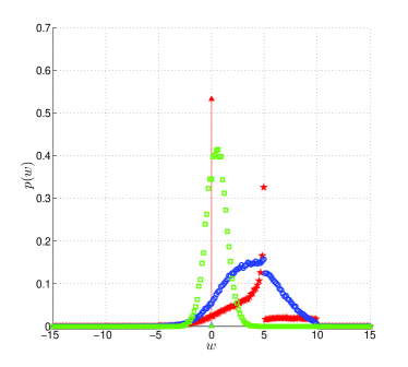
Figure 1: Work distributions $p(w)$ as obtained from the FATA for $\Delta E=V=5$ and $\omega=0.1$ (squares, green color), 1 (circles, blue color), and $\omega=10$ (stars, red color).

In current research of non-equilibrium systems, in particular of processes in small molecular systems, the investigation of distributions of microscopic work receives much attention. Among others, this is largely motivated by questions concerning the optimization of processes, and by the connection of the work distributions to fluctuation theorems. These theorems allow one to obtain equilibrium thermodynamic quantities from the study of non-equilibrium processes and they are useful for getting a deeper insight into the manifestation of the second law of thermodynamics. At the same time, the analytical expressions for the work distribution are rarely attainable (one exception is reported in Chvosta:2007 ). It is therefore interesting to see how the FATA can be employed for studies in this research field. To be specific, we focus on the stationary state and calculate work distributions within one period of the external driving. For these distributions we check the detailed fluctuation theorem of Crooks Crooks:1999 , as generalized by Hatano and Sasa Hatano/Sasa:2001 to steady states (for a nice summary of different forms of detailed and integral fluctuation theorems, see Esposito/VandenBroeck:2010 ).

In our model, due to the possibility of thermally activated transitions between the eight microstates, the state vector $\mathbf{n}$ must be understood as a stochastic process. We designate it as $\mathbf{n}(t)$, and let $\mathbf{n}^{{\rm tr}}(t)$ denotes its arbitrary fixed realization. The instantaneous energy of the compound system along this realization is then $H(\mathbf{n}^{{\rm tr}}(t),t)$. The work done on the system during the $m$th period $[m\tau,(m+1)\tau]$, $\tau=2\pi/\omega$, if the system evolves along the realization in question, is given by

$$w^{{\rm tr}}_{m} =\int_{m\tau}^{(m+1)\tau}dt\,\frac{\partial}{\partial t}H(\mathbf{n}^{{\rm tr}}(t),t)$$

$$=\frac{\omega\Delta E}{2}\sum_{i=1}^{3}\int_{m\tau}^{(m+1)\tau}dt\,n^{{\rm tr}}_{i}(t)\cos(\omega t)\,\,.$$ (17)

In the stationary limit $m\to\infty$ ($m\gg 1$) we can drop the index $m$. According to the detailed fluctuation theorem, the work distribution $p(w)$ should, in our case (time-symmetric situation with respect to the initial microstate distribution for starting forward and backward paths), obey the relation $p(w)\exp(-w)=p(-w)$.

Figure 1 shows the results for $p(w)$ obtained from the FATA for $\Delta E=V=5$, and three different frequencies $\omega=0.1$, 1, and 10. First, we let the system evolve during the $N_{{\rm ini}}=1$ ($\omega=0.1$), $N_{{\rm ini}}=3$ ($\omega=1$), $N_{{\rm ini}}=9$ ($\omega=10$) periods to reach the stationary state. Subsequently, the work values $w^{{\rm tr}}$ according to Eq. (17) were sampled over $N=10^{4}$ ($\omega=0.1$), $N=10^{5}$ ($\omega=1$), and $N=10^{5}$ ($\omega=10$) periods.

With decreasing $\omega$, the maxima of the work distributions in Fig. 1 shift toward $w=0$, and $\delta$-singularities, marked by the vertical lines, receive less weight. These $\delta-$singularities are associated with stochastic trajectories of the system, where no transitions occur within a period of the driving. For $\omega=0.1$, $p(w)$ is already close to the Gaussian fluctuation regime.

In Fig. 2 we show that the work distributions from Fig. 1 indeed fulfill the detailed fluctuation theorem. This demonstrates that the FATA successfully generates system trajectories with the correct statistics of the stochastic process.

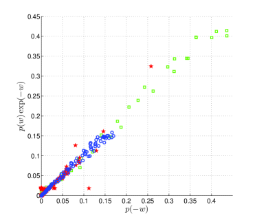
Figure 2: Check of the detailed fluctuation theorem $p(w)\exp(-w)=p(-w)$ for the work distributions shown in Fig. 1. The same symbols/colors are used for the three different frequencies as in Fig. 1.

IV Summary

In summary, we have presented new simulation algorithms for Markovian jump processes with time-dependent transition rates, which avoid the often cumbersome or unhandy calculation of inverse functions. The ATA and FATA rely on the construction of a series of Poisson points, where transitions are attempted and rejected with certain probabilities. As a consequence, both algorithms are easy to implement, and their efficiency will be good as long as the number of rejections can be kept small. For complex interacting systems, the FATA has the same merits as the FRTA with respect to the FRA. Both the ATA and FATA generate exact realizations of the stochastic process. Their connection to perturbative solutions of the underlying master equation may allow one to include in future work also non-Markovian features of a stochastic dynamics by letting the rejection probabilities to depend on the history Chvosta:1999 . Compared to the RTA and FRTA, the new algorithms should in particular be favorable, when considering periodically driven systems with interactions. Such systems are of much current interest in the study of non-equilibrium stationary states and we thus hope that our findings will help to investigate them more conveniently and efficiently.

- (1) Gibson, M. A. Bruck, J., J. Phys. Chem. A, 104 (2000) 1876.
- (2) Anderson, D. F., J. Chem. Phys., 127 (2007) 214107.
- (3) Astumian, R. D., Procl. Natl. Acad. Sci., 104 (2007) 19715.
- (4) Crooks, G. E., Phys. Rev. E, 60 (1999) 2721; ibid., 61 (2000) 2361.
- (5) Seifert, U., Phys. Rev. Lett., 95 (2005) 040602.
- (6) Esposito, M. Van den Broeck, C., Phys. Rev. Lett., 104 (2010) 090601.
- (7) Gillespie, D. T. J. Comput. Phys., 28 (1978) 395.
- (8) Bortz, A. B., Karlos, M. H. Lebowitz J. L., J. Comp. Phys., 17 (1975) 10.
- (9) Jansen, A. P. J., Comp. Phys. Comm., 86 (1995) 1.
- (10) Einax, M. Maass, P., Phys. Rev. E, 80 (2009) 020101(R).
- (11) Hatano, T. Sasa, S. I., Phys. Rev. Lett. 86 (2001) 3463.
- (12) Chvosta, P., Reineker, P. Schulz, M., Phys. Rev. E, 75 (2007) 041124.
- (13) Chvosta, P. Reineker, P., Physica A 268 (1999) 103.