Image Coaddition with Temporally Varying Kernels

Abstract

Large, multi-frequency imaging surveys, such as the Large Synaptic Survey Telescope (LSST), need to do near-real time analysis of very large datasets. This raises a host of statistical and computational problems where standard methods do not work. In this paper, we study a proposed method for combining stacks of images into a single summary image, sometimes referred to as a template. This task is commonly referred to as image coaddition. In part, we focus on a method proposed in Kaiser (2004), which outlines a procedure for combining stacks of images in an online fashion in the Fourier domain. We evaluate this method by comparing it to two straightforward methods through the use of various criteria and simulations. Note that the goal is not to propose these comparison methods for use in their own right, but to ensure that additional complexity also provides substantially improved performance.

1 Introduction

In astronomy today, the standard technique for acquiring deep astronomical images is through a series of short, often dithered, exposures. Applying this procedure enables the removal of cosmic rays, the filtering of bad pixels, and the masking of device defects. It also increases the dynamic range of the resulting image (as bright sources in single, long exposures saturate) and provides better control of the underlying point spread function (PSF) as long as the PSF is fully sampled.

To achieve the depth of a long exposure from a series of exposures requires that we combine the individual images, accounting for the variation in seeing, sky transparency, and background variability. This process is typically referred to as “image coaddition” and is at the heart of many image processing systems. The criteria that we optimize in the image coaddition depends on the science in question at hand. For example, in faint galaxy surveys (e.g. the Hubble Ultra Deep Field, Beckwith (2006)) photometric accuracy might be paramount, but for weak lensing surveys (e.g. the Canada France Hawaii Telescope Legacy Survey, Parker (2007)), the preservation of the underlying image resolution may be the primary concern. Given these differing objectives two open questions remain; how do we optimize the coaddition of astronomical images and is there is an optimal criterion that is relevant to all scientific goals?

With a new generation of deep imaging surveys coming on-line throughout this decade, including the Panoramic Survey Telescope & Rapid Response System (Pan-STARRS), the Dark Energy Survey (DES), and the Large Synoptic Sky Survey (LSST), each producing petabytes of data, image coaddition cannot just be assed by the statistical analysis; it is also a question of the computational efficiency of the different approaches. In this paper, we compare several different approaches for image coaddition, taking into account their statistical properties and their computational cost. We consider in detail the Fourier-domain methods proposed in Kaiser (2004) along with several straightforward methods, such as running means or medians. We compare these methods using two performance criteria: flux conservation (i.e., pixelwise photometric accuracy) and image resolution (using a metric we call Image Quality). Using these comparisons we can make statements about whether the additional complexity outweighs the extra costs they incur. Our goal is to provide a framework for assessing the magnitude of the practical advantages more complex methods might provide.

In Section 2, we set up the statistical model underlying our analysis and outline the properties of the various techniques. In Section 3, we describe the simulations and define the performance criteria, and, in Section 4, we present the results of our simulations.

1.1 Mathematical Setup

Consider a single image of a particular patch of sky. The object of interest is the true scene, which we represent as a function $g$ that takes a two-dimensional argument corresponding to position in the image and returns an intensity. For ground-based viewing, however, we observe only a blurred, discretized, and noisy version of $g$. We represent the blurring (caused by atmospheric seeing and instrument artifacts) by an operator $K$. In this case, $K$ is associated with a PSF $k$ such that the action of $K$ on $g$ is to integrate $g$ against $k$.

Now, suppose instead of getting one image we get a stack of $L$ images, all of the same patch of sky with science $g$. We assume for this discussion that the images have been registered. Then, due to atmospheric conditions changing over time, for each image $i$ there is a possibly different operator $K_{i}$ with associated PSF $k_{i}$. Then, if we define a regular grid of pixel centers $x_{1},x_{2},\ldots$, the observation on the $i^{th}$ image at the $j^{th}$ pixel is

$$Y_{ij}=\int k_{i}(x_{j},y)g(y)\,{\rm d}y\,+\,\epsilon_{ij},$$ (1)

where the $\epsilon_{ij}$’s are noise random variables with suitable distributions. Note that equation (1) also defines the operator $K_{i}$ as integrating $g$ against the PSF $k_{i}$. The statistical problem is to estimate $g$ given observation of $Y=(Y_{1},Y_{2},\ldots)$.

What makes the problem challenging is that the operators $K_{i}$ are ill conditioned, meaning that large changes in $g$ can make relatively small changes in $Y_{ij}$, making recovery of $g$ from $Y_{ij}$ unstable. This is so because blurring dampens high frequency structure, so the singular values of this integral operator decay quickly to zero. Thus, even small levels of noise can critically obscure structure in $g$.

To see this in a simple example, assume that the PSF does not vary in shape across the image, which makes $k(x,y)=k(x-y)$ a convolution kernel. It follows that by using the Fourier transform $\mathcal{F}$, we can recover $g$ exactly in the absence of noise by

$$g={\mathcal{F}}^{-1}\left(\frac{\mathcal{F}(Kg)}{\mathcal{F}k}\right)$$ (2)

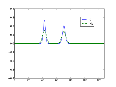
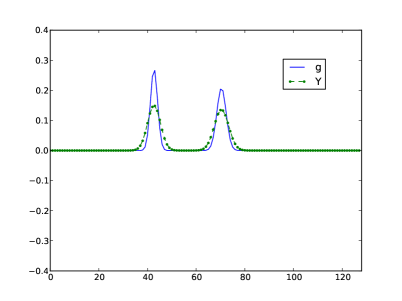
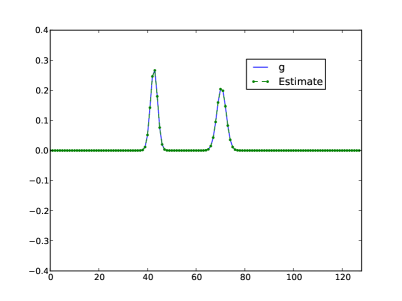
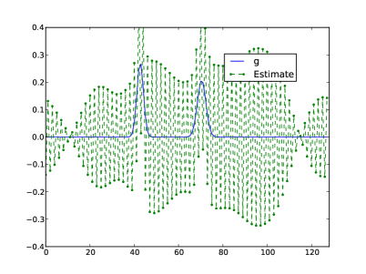
because $\mathcal{F}(Kg)=\mathcal{F}k\,\mathcal{F}g$. While the inverse exists in the absence of noise, the decay of $\mathcal{F}k$ at high frequencies can produce catastrophically high variances in the presence of noise, which produces nontrivial and random contribution at high frequencies (so the numerator is non-zero but the denominator goes to zero). Figure 1 demonstrates this effect in a 1-dimensional analog of the problem, comparing noise free reconstruction via equation (2) with reconstruction under noise with a 10e9:1 signal-to-noise ratio (SNR). The estimate in the latter case is wholly untenable.

(a) No Noise: Example

(b) 10e9:1 SNR: Example

(c) No Noise: Estimate

(d) 10e9:1 SNR: Estimate

Figure 1: We simulate a very simple case of a $g$ that is a mixture of two Gaussians, represented as blue, solid curves. We apply constant Gaussian seeing as well, which results in a new function $Kg$, displayed as a green, dashed curve. Then, we make observations at discrete, regular points, plotted as solid green dots. In (a) we observe $Kg$ directly and in (b) we observe $Kg$ under a miniscule amount of noise, 10e9:1 SNR. Using equation (2), we attempt to recover $g$ using these observations. These recoveries are in (c) and (d), respectively. Notice that we can perfectly reconstruct $g$ in absence of noise. However, even though $Y$ and $Kg$ are visually identical, the same inverse approach fails spectacularly in the second case.

1.2 Statistical Model

We assume that each observation is drawn from a distribution with mean

$$\theta_{ij}=(K_{i}g)(x_{j})=\int k_{i}(x_{j},y)g(y)\,{\rm d}y.$$ (3)

Because the observation process in the telescope involves counting photons, the distribution of $Y_{ij}$ is well modeled by a Poisson distribution (Hu, 2007; Scully, 1969). Thus, we assume that the $Y_{ij}$’s are independent Poisson$\langle\theta_{ij}\rangle$ random variables. If the mean counts $\theta_{ij}$ are large enough, the Gaussian approximation to the Poisson distribution is accurate, and we can model the $Y_{ij}$’s as independent Normal$\langle\theta_{ij},\theta_{ij}\rangle$ random variables.

The statistical problem is to form an estimator $\hat{g}$ of $g$ given observations $Y_{ij}$. In the present context, $\hat{g}$ is the template or coadd we are attempting to create. For each $\hat{g}$ we need ways to measure its misfit relative to the true scene $g$. In this paper we consider two. The first criteria corresponds to flux conservation, which we measure through Mean Integrated Squared Error (MISE), and the second criteria we refer to as Image Quality. We give a brief description of these here. See section 3 for a more thorough discussion.

Flux conservation gives an indication about how well a method maintains the spatial location of a given amount flux. Mean Integrated Squared Error (MISE), which corresponds to the expected value of the integrated squared difference between any recovered image and the true image $g$ is the measure of flux conservation we use. Specifically, suppose we form a template $\hat{g}$. Then

$$MISE(\hat{g},g)=\mathbb{E}\int(\hat{g}(x)-g(x))^{2}dx.$$

See Silverman (1985) for a thorough overview of MISE.

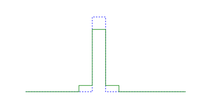
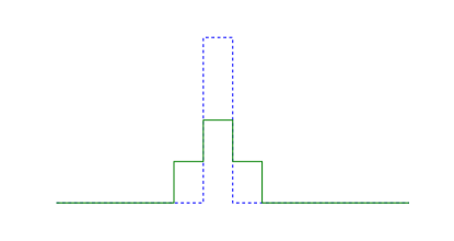
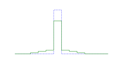
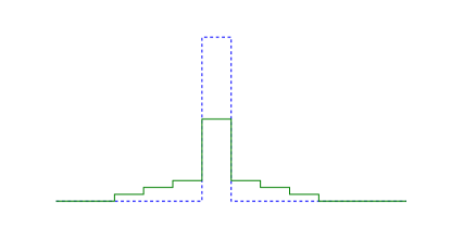
While MISE measures the degree to which $\hat{g}$ maintains flux in the correct location, it doesn’t distinguish between different scatterings of the remaining misspecified flux. We define a second comparison, which we call Image Quality, that is designed to measure how spread out the source is, as this isn’t captured by MISE. For Image Quality, we do a very rough PSF estimation on a source in the coadded image $\hat{g}$. The relative size of these PSFs give us an indication about how spread out an object gets by the coaddition. See Fig. 2 for an example of proceedures with combinations of good and bad MISE and Image Quality.

(a) Good MISE, Good Image Quality

(b) Bad MISE, Good Image Quality

(c) Good MISE, Bad Image Quality

(d) Bad MISE, Bad Image Quality

Figure 2: The dashed line represents the single pixel $\delta$-function of $g$. The solid line corresponds to a possible reconstruction. The first column has estimates that have good MISE and the first row has estimates that have good Image Quality. The second column and row have poor MISE and Image Quality, respectively.

One significant complication in practice is that the PSFs are unknown and must be estimated as part of the procedure. While it is ideal to simultaneously estimate the PSF and $g$, it is common, and typically effective, to first estimate the PSF and then use the estimate as a ’known’ PSF in the coaddition procedure. Because our focus is on the relative performance of techniques for estimating $g$, we will follow standard practices and assume that the PSFs are known. This produces a comparison of the techniques at their best but does not account for how well the procedures tolerate mis-estimation of the kernels. Note that the straightforward comparison methods do not require PSF estimates. So, any method that does require knowledge of the PSF would need to be substantially better, given it has access to much more information.

2 Methods

In this section, we describe a variety of methods that have been applied to the coaddition problem, with particular focus on the Fourier domain approach we are analyzing. Note that we restrict our attention to non-iterative methods.

Lucky Imaging. In lucky imaging, a large number of images are observed and only the ’best,’ according to some criterion such as seeing, are retained. Fried (1978) and Tubbs (2003) describe such implementations in detail. An advantage of this approach is that the reconstruction of the true scene is based entirely on high quality data. A disadvantage is that the method requires storing many images to determine which are best. Moreover, the images that are discarded can contain useful information about the scene that is, in effect, wasted.

Pixelwise Statistics. If a stack of images is aligned, the values at a particular pixel in each image represent a random sample from a common distribution. The aligned pixel stacks can thus be used to estimate the parameters of these distributions and in turn the true scene. Basic choices would be a mean, median, or perhaps a trimmed mean to account for heavy-tailed noise, but more sophisticated estimators tailored to particular distributional assumptions can be constructed. The advantages of these approaches are computational and conceptual simplicity. Moreover, the mean can be computed sequentially with a fixed amount of storage, although this is not true of the median or trimmed mean, for which the entire image stack needs to be maintained. A big disadvantage is that pixelwise methods tend to create rough, discontinuous images as no information sharing is permitted between pixels.

Fourier Deconvolution. In spatially constant seeing case is that equation (1) has a convolutional structure $k_{i}(x,y)\equiv k_{i}(x-y)$. The advantage of Fourier based methods is that the operator $K_{i}$ decomposes nicely in the Fourier domain. An inherent disadvantage to the Fourier approach is that great care must be used to avoid outcomes such as Fig. 1.

The approach outlined in Kaiser (2004) is to Fourier transform each image and estimate the $u^{th}$ Fourier coefficient of $g$ by a weighted average of the $u^{th}$ Fourier coefficient of each image. The weighting is accomplished so that the images with better seeing are weighted more heavily in the average. This method has some associated optimality properties. However, in practice, these properties turn out to not be useful. See below for a more thorough description.

Note that, as presented, this method makes three nontrivial assumptions. First, it assumes that each $k_{i}(x,y)\equiv k_{i}(x-y)$, that is, spatially constant seeing. As we describe in Section 4, while this assumption could have significant consequences when seeing varies spatially, in practice, it does not appear to cause much problem. The second assumption is that the $\theta_{ij}$’s are large enough that the Gaussian approximation to the Poisson is accurate across the image. The third assumption is that the variance of the Gaussian is a known value $\sigma^{2}_{i}$ that depends only on the image $i$. These last two assumptions make the analysis easier, and while they are often reasonable, they need not hold in practice.

To define the Fourier Deconvolution estimator, first expand $g$ into the Fourier basis, which we write as $(\phi_{u})$,

$$g=\sum_{u}\tilde{g}(u)\phi_{u}.$$ (4)

In general, we use the notation $\tilde{f}$ for the Fourier transform of the function $f$.

Using the above assumptions, and the resulting form of the $\theta_{ij}$’s, Kaiser (2004) proposes two estimators of $\tilde{g}(u)$. See Table 1 for these estimators and some of their cumulants. The first estimator in the table, $\widehat{\tilde{g}(u)}$, has the smallest variance of all unbiased estimators of $\tilde{g}(u)$. Also, the resulting estimator of $g$, defined to be

$$\hat{g}=\sum_{u}\widehat{\tilde{g}(u)}\phi_{u},$$ (5)

is the best linear unbiased estimator of $g$.

Estimator			Expectation & Variance
$\widehat{\tilde{g}(u)}$	$=$	$\frac{\left(\displaystyle\sum_{l=1}^{L}\frac{\overline{\tilde{k}_{l}(u)}\tilde{Y}_{l}(u)}{\sigma_{l}^{2}}\right)}{\left(\displaystyle\sum_{i=1}^{L}\frac{|\tilde{k}_{i}(u)|^{2}}{\sigma_{i}^{2}}\right)}$	$\mathbb{E}_{g}\left[\widehat{\tilde{g}(u)}\right]$	$=$	$\tilde{g}(u)$
			$\mathbb{V}_{g}\left[\widehat{\tilde{g}(u)}\right]$	$=$	$\frac{\displaystyle 1}{\left(\displaystyle\sum_{i=1}^{L}\frac{|\tilde{k}_{i}(u)|^{2}}{\sigma_{i}^{2}}\right)}$
$\widehat{\tilde{g}_{*}(u)}$	$=$	$\frac{\left(\displaystyle\sum_{l=1}^{L}\frac{\overline{\tilde{k}_{l}(u)}\tilde{Y}_{l}(u)}{\sigma_{l}^{2}}\right)}{\left(\sqrt{\displaystyle\sum_{i=1}^{L}\frac{|\tilde{k}_{i}(u)|^{2}}{\sigma_{i}^{2}}}\sqrt{\displaystyle\sum_{j=1}^{L}\frac{1}{\sigma_{j}s^{2}}}\right)}$	$\mathbb{E}_{g}\left[\widehat{\tilde{g}_{*}(u)}\right]$	$=$	$k^{*}(u)\tilde{g}(u)$
			$\mathbb{V}_{g}\left[\widehat{\tilde{g}_{*}(u)}\right]$	$=$	$\displaystyle\sum_{i=1}^{L}\frac{1}{\sigma_{i}^{2}}$

Table 1: $\tilde{k}^{*}(u):=\frac{\sqrt{\displaystyle\sum_{i=1}^{L}|\tilde{k}_{i}(u)|^{2}/\sigma_{i}^{2}}}{\sqrt{\displaystyle\sum_{j=1}^{L}1/\sigma_{j}^{2}}}$, which is the result of a variance stabilizing transformation.

However, as alluded to previously, these optimality properties are not useful. To see this, observe that the variance of $\hat{g}$ is the sum of the variances of $\widehat{\tilde{g}(u)}$. Also, since the $K^{\prime}s$ are smoothing operators, $|\tilde{k}(u)|$ is small for large $|u|$. In fact, the worse the seeing, the smaller $|\tilde{k}(u)|$ becomes and can be smaller than machine error in many cases. Hence, as $\mathbb{V}_{g}[\widehat{\tilde{g}(u)}]$ depends on the reciprocal of $|\tilde{k}(u)|$, the variance of $\hat{g}$ can be arbitrarily large. Note that we have seen a case of this already in Figure 1 where this large variance property causes unusable results.

Generally speaking, demanding unbiased estimators is less effective than choosing an estimator with some bias but smaller variance. In this case, the distinction is crucial because the unbiased estimator is unusable. For the interested reader, Chapter 7 of Wasserman (2006) provides a good introduction to this surprisingly broad and deep issue. See Figure 3 for an example of equation (5) in a simple simulated situation. The ability of $\hat{g}$ to reconstruct even a simple $g$ decays rapidly as the full width at half maximum, or FWHM, of the PSF increases. In particular, even the small amount of seeing (FWHM of 1.1 pixels) in the right most column makes the estimator unusable.

$\begin{array}[]{@{}c@{}c@{}c@{}}\includegraphics[width=144.54pt]{./kaiseropt_conv_low.eps}&\includegraphics[width=144.54pt]{./kaiseropt_conv_med.eps}&\includegraphics[width=144.54pt]{./kaiseropt_conv_high.eps}\\ \includegraphics[width=144.54pt]{./kaiseropt_low.eps}&\includegraphics[width=144.54pt]{./kaiseropt_med.eps}&\includegraphics[width=144.54pt]{./kaiseropt_high.eps}\\ \end{array}$

Figure 3: This is an example of the use of $\hat{g}$. The true scene $g$ is a one pixel delta function representing a star (not pictured). Top Row: An example of an input, or observed, image. Bottom Row: Reconstruction using $\hat{g}$. Left to Right: We increase the FWHM from 0.5 pixels to 1.1 pixels. Note that this means that some of the images have an undersampled PSF. This isn’t an issue in this case as we are applying the seeing ourselves and can without loss of generality assume the star is at the centroid of the pixel spike in $g$. The performance decays rapidly as the width of the seeing increases. In particular, even the mild amount of seeing in the right most column makes the estimator unusable. The magnified high frequency information has swamped the signal we wish to recover and left checkerboard pattern seen in the bottom right image..

Kaiser (2004) provides a correction that prevents the variance from exploding for large $|u|$ by multiplying $\widehat{\tilde{g}(u)}$ by a term that is proportional to the reciprocal of its standard deviation. See the second row of Table 1. This multiplication biases the estimator but bounds the variance. We define

$$\hat{g}_{*}=\sum_{u}\widehat{\tilde{g}_{*}(u)}\phi_{u}$$ (6)

and we spend the balance of the paper investigating its properties. We refer to $\hat{g}_{*}$ as the Fourier Deconvolution (FD) method. As an aside, since the correction corresponds to multiplication in Fourier space, we see that the bias of $\hat{g}_{*}$ is given by $(k^{*}*g)-g$, where the Fourier transform of $k^{*}$ is defined in the caption of Table 1 and $(a*b)$ is the convolution of $a$ and $b$.

2.1 Computational and Space Complexities

The computational complexity of the FD method is dominated by the need to Fourier transform the data and kernel. If we suppose the images are $m$ by $n$ and $N:=mn$, then we can perform a Fourier transform in $O(N\log N)$ FLOPs via the fast Fourier transform. This is the dominating computation in the FD method. However, it also has several order $O(N)$ computations. The mean method requires $2N$ FLOPs and the median method requires $N$ comparisons to update for each new image.

The FD method must maintain two $N$ pixel images and the mean method requires one $N$ pixel image, each of which get updated after each new image and kernel is recorded. The median method requires the entire stack must be maintained at all times, though not necessary in RAM. Hence, after $L$ images have been observed, all $L$ images must be kept for possible updating of the median.

3 Methods: Images and Evaluation Criteria

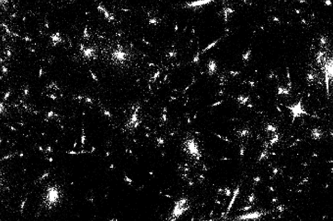
For our evaluation metrics, we need to know the true sky before any distortions. Hence, we simulate an idealized view of the sky (above the atmosphere) using a catalog of point and extend sources. Extended sources are represented by Sersic profiles and the density of point and extended sources is designed to match observations to a depth of r$\sim$28. Figure 4 shows a representation of one such image. From these true scenes, we apply a blurring operator $K$ and noise with variance $\sigma^{2}$ to represent the effect of the atmosphere, telescope, and instrument.

Under the assumptions of the FD method, we assume the PSFs are convolutional (by that we mean spatially constant seeing), but this leaves open the specific functional form for the kernel $k$. We choose to set $k$ to be the two dimensional Gaussian probability density function. Our results are, however, robust against more complicated parametrization of $k$ (e.g., a mixture of Gaussians).

Figure 4: The simulated image after being z-scaled and power transformed. The pixel width of this simulation is 0.2 arcsec (0.2”).

For evaluating the effectiveness of the FD method, we compare it to the pixel-wise mean and pixel-wise median. Our goal is to assess the value added by the FD method and evaluate whether the improved performance overcomes the added cost and complexity of the method. The mean and median procedures are intended as extreme comparisons rather than serious proposals and we aren’t endorsing their use in this paper. However, if the value added of more sophisticated methods relative to even these simplistic methods is not great, then it suggests that simple methods may suffice in practice. Note that the computational complexity of the methods is not a purely academic concern. In large imaging surveys such as the LSST, a near constant data stream requires efficient, near real-time processing, and the cost of generating template images is an important factor.

For this comparison, we use the two general criteria introduced in section 1.2 corresponding to MISE and Image Quality. In principle, at least two different errors can be made when comparing an estimated template $\hat{g}$ to the true scene $g$. These errors can most easily be thought of in the context of a point source such as a star. Our estimated image can remove some of the flux from the point source and/or it can smooth the image (degrading the photometric accuracy and the resolution of the resulting template). Figure 2 shows examples of a pixelated point source that has been reconstructed by four made-up methods.

In the MISE comparison we compute the expected value of the integrated squared difference between the true image and our estimate, assuming zero background. Under the non-Gaussian distributions, a larger variance results in more total flux in the image. This, in turn, results in a large MISE. To compensate for this increase, and to make all the cases more directly comparable, we rescale the MISE by the total signal of each image to compensate for this additional flux.

For the evaluation of Image Quality we fit a two dimensional, spherical Gaussian density to a source using least squares. The covariance matrix of this fitted Gaussian is then used as a metric for the width of the point source.

4 Results

In this section, we present the results of our simulations. The section is divided into two parts, corresponding to the two evaluation criteria outlined above.

4.1 MISE

When looking at equation (1) we see two major influences on the quality of the observation. One is the type and severity of the seeing, determined by the PSF $k$. The other is the distribution of the noise $\epsilon$. In this section, we look at several different scenarios for comparing the mean or median to the FD method by changing these two factors.

4.1.1 Increasing FWHM Comparison

Overall, we wish to understand the impact of seeing and noise on the performance of the methods. To do this, we simulate a stack of images with each image having a FWHM drawn from a distribution with mean, $\mu_{FWHM}$. We do this procedure for $\mu_{FWHM}$ ranging from 2 pixels to 7 pixels (0.4” to 1.4”). This interval is chosen so that it contains the expected seeing width for the LSST. This procedure creates a sequence of stacks of images.

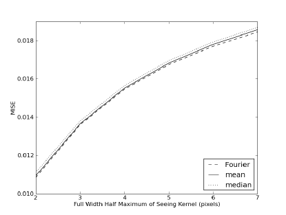
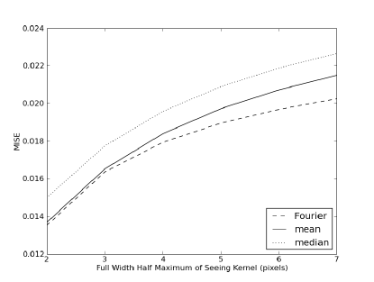
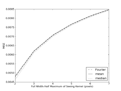
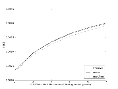
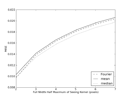
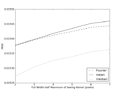
We apply this increasing FWHM to six different noise parameterizations. For both high variance (5:1 SNR) and low variance (20:1 SNR) we have the noise term be distributed Gaussian, heavy-tailed shot, and inhomogeneous Poisson noise. In all six combinations, a lower MISE indicates that the method conserved the flux better, on average. See Figure 5 for the results.

In all cases, the mean severity of seeing, $\mu_{FWHM}$, does not impact the ranking of the methods. In the Gaussian case, the methods are ranked, from best to worst, as FD, mean, and then median. In both the low and high noise cases, absolute difference between the mean and the median is constant for all levels of $\mu_{FWHM}$ due to the well-known efficiency gains of the mean over the median in the Gaussian case. However, in the high noise case, the difference in MISE between the FD and mean methods increases 11% as $\mu_{FWHM}$ ranges from 2 to 7 pixels. As the FD method uses the additional information of a known seeing kernel, this non-constant difference is expected.

In the inhomogeneous Poisson or heavy-tailed shot noise cases, the median outperforms both other methods. This owes to the particular and well known feature of the median to be more robust against heavier-tailed distributions. In the shot-noise case, the median ignores the random noise spikes with overwhelming probability and we get a noise free version of the true scene $g$ with the median amount of seeing. The very small advantage of the FD over the mean method owes to the FD’s slightly narrower impulse response function, which we discuss in section 4.2 and Figure 7. In the inhomogeneous Poisson noise case, the observed image is created by simulating independently from a Poisson$\langle\theta_{ij}+\sigma^{2}\rangle$ from equation (3). This creates a very noisy image, especially near sources, and hence the median’s ability to ignore large, transient spikes results in the large MISE advantage.

Under all three noise distributions, the FD method displays a small but increasing benefit in flux conservation over the mean as $\mu_{FWHM}$ goes from 2 to 7. It should be kept in mind that the FD method uses the known kernel assumption. Hence, as the seeing becomes more severe this informational advantage should become more pronounced. In reality, the kernel would need to be estimated and this advantage would most likely decay.

(a) Gaussian, Low Noise

(b) Gaussian, High Noise

(c) Shot, Low Noise

(d) Shot, High Noise

(e) Inhomogeneous Poisson, Low Noise

(f) Inhomogeneous Poisson, High Noise

Figure 5: Results for the MISE comparison. The “Low Noise” and “High Noise” are 20:1 and 5:1 signal to noise, respectively. Notice that the FD method slightly outperforms the mean and median under the Gaussian assumption. However, the median, being more robust to heavier-tailed distributions, dominates in the other two regimes.

4.2 Image Quality

To do this comparison we use an image where the function $g$ is a $\delta$-function (i.e. a point source). We use the expected distribution of seeing at the LSST stack to draw 10 independent and identically distributed Gaussian PSFs and apply them to the point source. This mimics the forward process of an image getting blurred by the atmosphere and corresponds to operating on $g$ with $K_{i}$ for $i=1,2,\ldots,10$. For this stack of images we apply the three methods described earlier, FD, mean, and median, to derive a template image. We then fit a spherical Gaussian kernel to the template via least squares and use the diagonal element of the covariance matrix as a measure of the width of the method’s PSF.

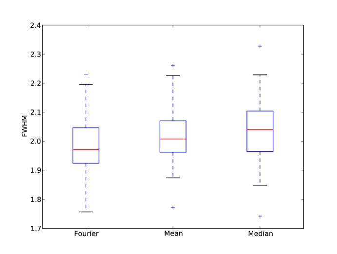
We make 1000 draws from the seeing distribution and compute this statistic for each method and each draw. The results are summarized in Figure 6 with boxplots of the FWHM of the fitted Gaussian kernel. Boxplots are a graphical tool for quickly conveying the distribution of observed data and are composed of a ‘box’ and ‘whiskers.’ The ‘box’ is the main rectangle, which has horizontal lines, increasing with FWHM, at the 25th, 50th, and 75th percentiles of the data. The ‘whiskers’ correspond to the dotted vertical lines with horizontal lines at the end and the plus signs. These horizontal lines are at the 1st and 99th percentile. The pluses are at extreme data points.

The boxplots are very similar and show little difference in the FWHM of the fitted kernels. The FD method has longer ‘whiskers’ than the other methods, indicating a wider range of fitted FWHM that can be expected. It also has a very slightly lower ‘box’ than the other two methods, indicating that the majority of draws result in a slightly better fitted FWHM. For instance, the 50th percentile of the FD method’s fitted FWHM is 1.2% lower then the mean method’s fitted FWHM.

Interestingly, one of the draws resulted in six very good seeing images and four poor images. This resulted in the median method having the smallest fitted FWHM recorded for any method on any draw. This is part of a more general property of the median to behave non-continuously with the composition of the stack. For instance, if there were instead 4 very good seeing images and 6 poor seeing images, the result would be a large fitted FWHM.

Figure 6: Boxplots of the FWHM of the fitted Gaussian kernel for stacks created from draws from the expected seeing distribution of the LSST site. The three methods considered in this paper are shown. The boxplots are very similar and show little difference in the FWHM of the fitted kernels.

4.2.1 Differences in Expectation

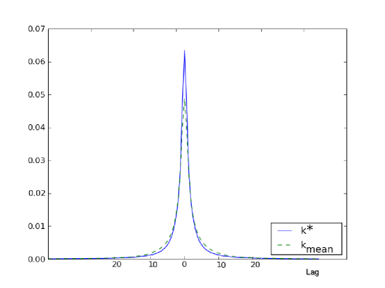
The mean and FD methods are very similar in that they are both based around summing the images and hence are both linear filters on the observed images. Let’s denote the estimated coadds of the two methods as $\hat{g}_{mean}$ and $\hat{g}_{*}$, respectively. We can understand the filtering that we are applying to the true image $g$ by considering $\mathbb{E}[\hat{g}_{mean}]$ and $\mathbb{E}[\hat{g}_{*}]$. Note that these are

$$\mathbb{E}[\hat{g}_{mean}]=\left(\frac{1}{L}\sum_{i=1}^{L}K_{i}\right)g=\int k_{mean}(x-y)g(y)dy\qquad\textrm{and}\qquad\mathbb{E}[\hat{g}_{*}]=\int k^{*}(x-y)g(y)dy$$ (7)

where the Fourier transform of the function $k^{*}$ is defined in the caption under Table 1.

By examining the impulse response functions (IRFs) of these filters we can find the average width of the PSFs that will result from these methods. Note that in this case this corresponds to the bias of each method. See Figure 7 for a one dimensional representation of the IRFs of the expected filters. The mean IRF and the Fourier Deconvolution IRF are virtually identical and would create no visible difference in the image quality.

Figure 7: This figure shows the IRF of the expected filter for the mean (dashed line) and FD (solid line) methods. Though $k^{*}$ has more mass at lag = 0, bear in mind that it uses a weighting scheme that depends on knowledge of both the true PSFs and true variances. Taking this into consideration, the difference is slight.

5 Discussion

A variety of template generation/image coaddition techniques have been applied in current imaging surveys, including the CFHTLS (Gwyn (2008); mean technique), PanSTARRS (Price (2007), mean technique), MOPEX for SIRTF images (Makovoz (2005), mean and median technique), and the VIRMOS survey (Radovich (2004), median technique). In this paper, we address the broad question of whether sophisticated methods of template generation and image coaddition are worth the added cost and complexity, in the context of modern image surveys with large and nearly constant data streams. To this end, we compare Fourier domain reconstruction techniques which have a variety of nice theoretical properties to straightforward pixelwise statistics. We consider two cost metrics to evaluate the image reconstructions; Image Quality by way of the resulting Gaussian FWHM of an image and the conservation of flux, measured by MISE.

Under the assumptions that motivate the FD method, namely Gaussian noise and spatially constant seeing, the FD and mean methods both have lower MISE than the median. However, in the heavy-tailed shot and inhomogeneous Poisson noise cases, the median outperforms the FD method.

In situations when there is a small amount of seeing in an image stack, corresponding to $\mu_{FWHM}\approx 2$ pixels, we see the mean and FD methods have nearly the same MISE properties (less than 0.7% difference across all considered noise distributions). However, as the severity of the seeing increases, the disparity between the methods increases as well. As the FD method incorporates knowledge of the seeing kernel, this property is to be expected. However, the MISE for the high noise Gaussian, shot, and inhomogeneous Poisson cases are only 5.4%, 1.2%, and 0.13% lower, respectively, at the most severe levels of seeing.

These benefits are rather small, particularly in the more realistic heavy-tailed and Poisson noise cases. This is especially so considering the extra computational complexities involved in the FD method over the mean and median methods.

For comparing image quality of the templates, we find that the resolution of the resulting images is very similar as the 50th percentile of the fitted FWHM of the FD method is less than 2% smaller than the 50th percentile of the fitted FWHM of the mean method.

We find that the value added by the FD method over the mean or median procedures does not overcome its added cost and complexity. This leads us to the conclusion that there is room for improvement over all three methods. We are currently exploring various possible improvements and theoretical justifications for some of the approaches outlined in this paper.

References

- Beckwith (2006) Beckwith, Steven et al., 2006, AJ, 132, 5, pg. 1729
- Fried (1978) Fried, D.L., 1978, J. Optical Soc. Amer, 86, pgs. 1651-1657
- Gwyn (2008) Gwyn, S. D. J., 2008, PASP, Feb., 120, pgs. 212-223
- Hu (2007) Hu, Yuchng et al., 2007, Physics Letters A, 367, pgs. 173-176
- Kaiser (2004) Kaiser, Nick, 2004, Private communication
- Makovoz (2005) Mokovoz, D. et al., 2005, Astronomical Data Analysis Software and Systems XIV, 347, Dec, pg. 81
- Parker (2007) Parker, Laura et al., 2007, ApJ, 669, 1, pg. 21
- Price (2007) Price, P.A and Pan-STARRS Team, Bulletin of the American Astronomical Society, 38, May, pg. 183
- Radovich (2004) Radovich M. et al., 2004, A&A, Apr., 417, pgs. 51-60
- Scully (1969) Scully, Marlan et al., 1969, Physics Review. 179, pgs. 368-374
- Silverman (1985) Silverman, Brian, 1985, Chapman & Hall/CRC, Monographs on Statistics and Applied Probability, Vol 26
- Tubbs (2003) Tubbs, R.N., 2003, PhD thesis, Cambridge Univ
- Wasserman (2006) Wasserman, Larry, 2006, Chapter 7, Springer Science