Modeling Image Structure with Factorized Phase-Coupled Boltzmann Machines

Abstract

We describe a model for capturing the statistical structure of local amplitude and local spatial phase in natural images. The model is based on a recently developed, factorized third-order Boltzmann machine that was shown to be effective at capturing higher-order structure in images by modeling dependencies among squared filter outputs [1]. Here, we extend this model to $L_{p}$-spherically symmetric subspaces. In order to model local amplitude and phase structure in images, we focus on the case of two dimensional subspaces, and the $L_{2}$-norm. When trained on natural images the model learns subspaces resembling quadrature-pair Gabor filters. We then introduce an additional set of hidden units that model the dependencies among subspace phases. These hidden units form a combinatorial mixture of phase coupling distributions, concentrated in the sum and difference of phase pairs. When adapted to natural images, these distributions capture local spatial phase structure in natural images.

1 Introduction

In recent years a number of models have emerged for describing higher-order structure in images (i.e., beyond sparse, Gabor-like decompositions). These models utilize distributed representations of covariance matrices to form an infinite or combinatorial mixture of Gaussians model of the data [2, 1]. These models have been shown to effectively capture the non-stationary variance structure of natural images. A variety of related models have focused on the local radial (in vectorized image space) structure of natural images [3, 4, 5, 6, 7]. While these models represent a significant step forwards in modeling higher-order natural image structure, they only implicitly model local phase alignments across space and scale. Such local phase alignments are implicated as being a hallmark of edges, contours, and other shape structure in natural images [8]. The model proposed in this paper attempts to extend these models to capture both amplitude and phase in natural images.

In this paper, we first extend the recent factorized, third-order Boltzmann machine model of Ranzato & Hinton [1] to the case of $L_{p}$-spherically symmetric distributions. In order to directly model the dependencies among local amplitude and phase variables, we consider the restricted case of two-dimensional subspaces with $L_{2}$-norm. When adapted to natural images, the subspace filters converge to quadrature-pair Gabor-like functions, similar to previous work [7]. The dependencies among amplitudes are modeled using a set of hidden units, similar to Ranzato & Hinton [1]. Phase dependencies between subspaces are modeled using another set of hidden units as a mixture of phase coupling “covariance” matrices: conditioned on the hidden units, phases are modeled via a phase-coupled distribution [9].

1.1 Modeling Local Amplitude and Phase

Our model may be viewed within the same framework as a number of recent models that attempt to capture higher-order structure in images by factorizing the coefficients of oriented, bandpass filters [3, 4, 5, 6, 7, 10, 11]. These models are currently the best probabilistic models of natural image structure: they produce state-of-the-art denoising [3], and achieve lower entropy encodings of natural images [5]. They can be viewed as sharing a common mathematical form in which the filter coefficients, $x$, are factored into a non-negative component $z$ and a scalar component $u$, where $x=z\,u$. The non-negative factors, $z$, are modeled as either an independent set of variables each shared by a pair of linear components [7], a set of variables with learned dependencies to the linear components [6], or as a single radial component [5, 4]. The scalar factor, $u$, is modeled in a number of ways: as an independent angular unit vector [5, 4], as a correlated noise process [3], as the phase angle of paired filters [7], or as a sparse decomposition of latent variables [10].

By separating the filter coefficients into two sets of variables, it is possible for higher levels of analysis to model higher-order statistical structure that was previously entangled in the filter coefficients themselves. For example, the non-negative variables $z$ are usually related to the local contrast or power within an image region, and Karklin & Lewicki have shown that it is possible to train a second layer to learn the structure in these variables via sparse coding [10]. Similarly, Lyu & Simoncelli learn an MRF model on these variables and show that the resulting model achieves state-of-the-art denoising [3]. It is generally less clear what structure is represented in the scalar variables $u$. Here we take inspiration from Zetzsche’s observations regarding the circular symmetry of joint distributions of related filter coefficients and conjecture that this quantity should be modeled as the sine or cosine of an underlying phase variable, i.e., $u=\sin(\theta)$ or $u=\cos(\theta)$ [12].

One of the main contributions of this paper is a model of the joint structure of local phase in natural images. For the case of phases in a complex pyramid, the empirical marginal distribution of phases is always uniform across a corpus of natural images (data not shown); however, the empirical distribution of pairwise phase differences is often concentrated around a preferred phase. We can write the joint distribution of a pair of phase variables with a dependency in the difference of the phase variables as a von Mises distribution in the difference of the phases:

$$p(\theta_{i},\theta_{j})=\frac{1}{2\pi I_{0}(k)}\exp(\kappa\cos(\theta_{i}-\theta_{j}-\mu))$$ (1)

This distribution is parameterized by a concentration $\kappa$ and a phase offset $\mu$. Using trigonometric identities we can re-express the cosine of the difference as a sum of bivariate terms of the form $\cos(\theta_{i})\sin(\theta_{j})$. One may view these terms as the pairwise statistics for angular variables, just as the the bivariate terms in the covariance matrix are the pairwise statistics for a Gaussian. This logic extends to multivariate distributions with $n>2$.

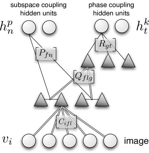
In the next section we describe an extension to the mean and covariance Restricted Boltzmann Machine (mcRBM) of Ranzato & Hinton [1]. Our extension represents local amplitude and phase in its factors. We model the amplitude dependencies with a set of hidden variables, and we model the phase dependencies among factors as a combinatorial mixture of phase-coupling distributions [9]. This model is shown schematically in Fig. 1.

Figure 1: The mpkRBM model is shown schematically. The visible units $v_{i}$ are connected to a set of factors through the matrix $C_{ifl}$. These factors come in pairs, as indicated by the horizontal line linking neighboring triangles. The squared output of each factor connects to the subspace coupling hidden units $h_{n}^{p}$ through the matrix $P_{fn}$. Another set of factors is connected to the sine and cosine representations of each factor (second layer triangles) through the matrix $Q_{flg}$. This second set of factors connects to the phase coupling hidden units $h_{t}^{k}$. Single-stroke vertical lines indicate linear interactions, while double stroke lines indicate quadratic interactions. Note that the mean factors, $h^{m}$, and biases are omitted for clarity. See text for further explanation.

2 Model

We first review the factorized third-order Boltzmann machine of Ranzato and Hinton [1] named mcRBM because it models both the mean and covariance structure of the data. We then describe an extension that models pairs of factors as two dimensional subspaces, which we call the mpRBM. The mpRBM provides a phase angle between pairs. The joint statistics between phase angles are not explicitly modeled by the mpRBM. Thus we propose additional hidden factors that model the pair-wise phase dependencies as a product of phase coupling distributions. For convenience we name this model mpkRBM, where k references the phase coupling matrix $K$ that is generated by conditioning on the phase-coupling hidden units.

2.1 mcRBM

The mcRBM defines a probability distribution by specifying an energy function E. The probability distribution is then given as $p(v)\propto\exp(-E(v))$, where $v\in R^{D}$ is the vectorized input image patch with $D$ pixels. The mcRBM has two major parts of the energy, the covariance contributions, $E^{c}$, and the mean contributions, $E^{m}$.

The covariance terms are defined as:

$$E^{c}(v,h^{c})=-\frac{1}{2}\sum_{n=1}^{N}h^{c}_{n}\sum_{f=1}^{F}P_{fn}(\sum_{i=1}^{D}C_{if}\frac{v_{i}}{||v||})^{2}-\sum_{n=1}^{N}b_{n}^{c}h_{n}^{c}$$ (2)

where $P\in R^{F\times N}$ is a matrix with positive entries, $N$ is the number of hidden units and $b^{c}$ is a vector of biases. The columns of the matrix $C\in R^{D\times F}$ are the image domain filters and their squared outputs are weighted by each row in $P$. The $P$ matrix can be considered as a weighting on the squared outputs of the image filters. We normalize the visible units ($||v||_{L_{2}}=1$) following the procedure in [1]. Each term in the first sum includes two visible units and one hidden unit and is a third-order Boltzmann machine. However, the third-order interactions are restricted by the form of the model into factors. Each factor, $(\sum_{i=1}^{D}C_{if}v_{i})^{2}$ is a deterministic mapping from the image domain. The hidden units combine combinatorially to produce a zero-mean Gaussian distribution with an inverse covariance matrix that is a function of the hidden units:

$$\Sigma^{-1}=C\,\mathrm{diag}(Ph^{c})C^{\prime}$$ (3)

Because the representation in the hidden units is distributed, the model can describe a combinatorial number of covariance matrices.

The mean contribution to the energy, $E^{m}$ is given as:

$$E^{m}(v,h^{m})=-\sum_{j=1}^{M}h^{m}_{j}\sum_{i=1}^{D}W_{ij}v_{i}-\sum_{j=1}^{M}b_{j}^{m}h_{j}^{m}$$ (4)

with $M$ binary hidden units $h_{j}^{m}$ that connect directly to the visible units through the matrix $W_{ij}$. The $b_{j}^{m}$ terms are the mean hidden biases. The form of the mean contribution is a standard RBM [13]. Note that the conditional over both sets of hidden units is factorial.

The conditional distribution over the visible units given the hidden units is a Gaussian distribution, which is a function of the hidden variable states:

$$p(v|h^{c},h^{m})\sim N(\Sigma(\sum_{j=1}^{M}W_{ij}h^{m}_{j}),\Sigma)$$ (5)

where $\Sigma$ is given as in Eq. 3. The mean of the specified Gaussian is a function of both the mean $h^{m}$ and covariance $h^{c}$ hidden units.

The total energy is given by:

$$E(v,h^{c},h^{m})=E^{c}(v,h^{c})+E^{m}(v,h^{m})+\frac{1}{2}\sum_{i=1}^{D}v_{i}^{2}-\sum_{i=1}^{D}b_{i}^{v}v_{i}$$ (6)

with the last two terms a penalty on the variance of the visible units introduced because $E^{c}$ is invariant to the norm of the visible units and biases $b_{i}^{v}$ on the visible units.

2.2 mpRBM

A number of recent results indicate that the local structure of image patches is well modeled by $L_{p}$-spherically symmetric subspaces [6]. To produce $L_{p}$-spherically symmetric subspaces we impose a pairing of factors into an $L_{p}$ subspace. The covariance energy term in the mcRBM is thus altered to give:

$$E^{p}(v,h^{p})=-\frac{1}{2}\sum_{n=1}^{N}h^{p}_{n}\sum_{f=1}^{F}P_{fn}\left[\sum_{l}^{L}(\sum_{i=1}^{D}C_{ifl}\frac{v_{i}}{||v||})^{\alpha}\right]^{1/\alpha}-\sum_{n=1}^{N}b_{n}^{c}h_{n}^{c}$$ (7)

Now the tensor $C_{ifl}$ is a set of filters for each factor, $f$ spanning the $L$ dimensional subspace over the index $l$. The distribution over the visible conditioned on the hidden units can be expressed as a mixture of $L_{p}$ distributions. Note that the hidden units remain independent conditioned on the visible units.

The optimal choice of $L$ and $\alpha$ is an interesting project related to recent models [14] but is beyond the scope of this paper. Here, we have chosen to focus on modeling the structure in the space complementary to the norms of the subspaces. To achieve a tractable form of the subspace structure we select the special case of $L=2$ and $\alpha=2$. The choice of $\alpha=2$ is motivated by subspace-ICA models [6] and sparse coding with complex basis functions [7] where the amplitude within each complex basis function subspace is modeled as a sparse component.

2.3 mpkRBM

While the formulation of $L_{p}$-spherically symmetric subspace models the spherically symmetric distributions of natural images, there are likely to be residual dependencies between the subspaces in the non-radial directions. For example, elongated edge structure will produce dependencies in the phase alignments across space and through spatial scale [8]. Such dependencies are not captured, or are at least only implicitly captured in the mpRBM. By formulating the mpRBM with $L=2$ and $\alpha=2$ we can define a phase angle within each subspace. The dependencies between these phase angles will capture image structure such as phase alignments due to edges. We define a new variable, $x_{fl}$, which is a deterministic function of the visible units: $x_{f1}=\cos(\theta_{f})$ and $x_{f2}=\sin(\theta_{f})$, where $\theta_{f}=\arg{\left((\sum_{i=1}^{D}C_{if1}v_{i})+\mathbf{j}(\sum_{i=1}^{D}C_{if2}v_{d})\right)}$, and $\mathbf{j}$ is the imaginary unit and $\arg(.)$ is the complex argument or phase.

We now use a mathematical form that is similar to the covariance model contribution in the mcRBM to model the joint distribution of phases. We define the energy of the phase coupling contribution, denoted $E^{k}$, as,

$$E^{k}(v,h^{k})=-\frac{1}{2}\sum_{t=1}^{T}h^{k}_{t}\sum_{g=1}^{G}R_{gt}(\sum_{l=1}^{L}\sum_{f=1}^{F}Q_{flg}x_{fl})^{2}-\sum_{t=1}^{T}b_{t}^{k}h_{t}^{k}$$ (8)

with $T$ binary hidden units $h_{t}^{k}$ that modulate the columns of the matrix $R\in R^{G\times T}$. The rows of R then modulate the squared projections of the vector $x$ through the matrix $Q\in R^{F\times L\times G}$. The term $b_{t}^{k}$ is a vector of biases for the $h_{t}^{k}$ hidden units. Similar to the $h^{c}$ terms in the mcRBM, the $h_{k}$ units in the mpkRBM contribute pair-wise dependencies in the sine-cosine space of the phases. Pair-wise dependencies in the sine-cosine space can be re-expressed using trigonometric identities as terms in the sums and differences of the phase pairs, identical to the phase coupling described in Eq. 1. Such explicit dependencies may be important to model because edges in images exhibit structured dependencies in the differences of local spatial phase.

Because the phase coupling energy is additive in each $h^{k}_{t}$ term the hidden unit distribution conditioned on the hidden units is factorial. The probability of a given $h^{k}_{t}$ is given as:

$$p(h^{k}_{t}|v)=\sigma\left(\frac{1}{2}\sum_{g=1}^{G}R_{gt}(\sum_{l=1}^{L}\sum_{f=1}^{F}Q_{flg}x_{fl})^{2}+b_{t}^{k}\right)$$ (9)

where the sigmoid, or logistic, function is $\sigma(y)=(1+\exp(-y))^{-1}$.

We can see the dependency structure imposed by the $h^{k}$ units by considering the conditional distribution in the space of the phases, $\theta$:

$$K=Q\,\mathrm{diag}(Rh^{k})Q^{\prime}$$

$$p(\theta|h^{k})\propto\exp(-\scriptstyle\frac{1}{2}\displaystyle x^{\prime}Kx)$$ (10)

Therefore, the $h^{k}$ units provide a combinatorial code of phase-coupling dependencies. The number of phase-coupling matrices that the model can generate is exponential in the number of $h^{k}$ hidden units because the hidden unit representation is binary and combinatorial. Again, instead of allowing arbitrary three way interactions between the $x$ variables and the hidden units, we have chosen a specific factorization where the squared factors are $(\sum_{l=1}^{L}\sum_{f=1}^{F}Q_{flg}x_{fl})^{2}$. Because there are no direct interactions between the hidden units, $h^{k}$, the model still has the form of a conventional Restricted Boltzmann Machine. We call this model a mpkRBM because it builds upon the mpRBM and the k references the coupling matrix in the pair-wise phase distribution produced by conditioning on $h^{k}$.

Combining the three types of hidden units, $h^{p}$, $h^{m}$, and $h^{k}$, allows each type of hidden unit to model structure captured by the corresponding functional form. For example, the $h^{p}$ hidden units will generate phase dependencies implicitly through their activations. However, if the phase structure of the data contains additional structure not captured implicitly by the $h^{p}$ and $h^{m}$ hidden units, there will be a learning signal for the $h^{k}$ units. Conversely, the phase statistics that are produced implicitly by the $h^{p}$ and $h^{m}$ units will be ignored by the $h^{k}$ terms because the learning signal is driven by the differences in the data and model distributions.

3 Learning

We learn the parameters of the model by stochastic gradient ascent of the log-likelihood. We express the likelihood in terms of the energy with the hidden units integrated out (omitting the visible squared term and biases):

$$F(v)= - \sum_{n=1}^{N}\log(1+\exp(\frac{1}{2}\sum_{f=1}^{F}P_{fn}\left[\sum_{l}^{L}(\sum_{i=1}^{D}C_{ifl}\frac{v_{i}}{||v||})^{\alpha}\right]^{1/\alpha}+b_{n}^{c}))$$

$$- \sum_{t=1}^{T}\log(1+\exp(\frac{1}{2}\sum_{g=1}^{G}R_{gt}(\sum_{l=1}^{L}\sum_{f=1}^{F}Q_{flg}x_{fl})^{2}+b_{t}^{k}))$$

$$- \sum_{j=1}^{M}\log(1+\exp(\sum_{i=1}^{D}W_{ij}v_{i}+b_{j}^{m}))$$

It is not possible to efficiently sample the distribution over the visible units conditioned on the hidden units exactly (in contrast, sampling from the visible units conditioned on the hidden units in a standard RBM is efficient and exact). We choose to integrate out the hidden variables, instead of taking the conditional distribution, to achieve better estimates of the model statistics.

Maximizing the log-likelihood the gradient update for the model parameters (denoted as $\Theta\in\{R,Q,b^{k},C,P,b^{c},W,b^{m},b^{v}\}$ is given as:

$$\frac{\partial L}{\partial\Theta}=\langle\frac{\partial F}{\partial\Theta}\rangle_{model}-\langle\frac{\partial F}{\partial\Theta}\rangle_{data}$$ (12)

where $\langle.\rangle_{\rho}$ indicates the expectation taken over the distribution $\rho$ . Calculating the expectation over the data distribution is straightforward. However, calculating the expectation over the model distribution requires computationally expensive sampling from the equilibrium distribution. Therefore, we use standard techniques to approximate the expectation of the gradients under the model distribution following the procedure in [15, 1]. To summarize, in Contrastive Divergence learning [13] the model distribution is approximated by running a dynamic sampler starting at the data for only one step. Given the energy function with the hidden units integrated out, we run hybrid Monte Carlo sampling [16] starting at the data for one dynamical simulation to produce an approximate sample from the model distribution. For each dynamical simulation we draw a random momentum and run 20 leap-frog steps while adapting the step size to achieve a rejection rate of about  10%.

Figure 2: Learned $L_{p}$ Weights, $C$: A) and B) show the individual components of each filter pair $C_{if1}$ and $C_{if2}$, respectively. Each subimage shows the image domain weights in the unwhitened color image space. C) shows the amplitude $\sqrt{(C_{if1}^{2}+C_{if2}^{2})}$ as a function of space, and D) shows the phase $\mathrm{arg}(C_{if1}+iC_{if2})$ as a function of space. Each panel preserves the ordering such that the image in position (1,1) of A) corresponds to the same subspace of $C$ as the image in position (1,1) of B), C), and D).

3.1 Learning parameters

We trained the models on image patches selected randomly from the Berkeley Segmentation Database. We subtracted the image mean, and whitened 16x16 color image patches preserving 99% of the image variance. This resulted in $D=138$ visible units. We examined a model with 256 $h^{c}$ covariance units, 256 $h^{k}$ phase-coupling units, and 100 $h^{m}$ mean units. We initialized the values of the matrix $C$ to random values and normalized each image domain vector to have unit length. We initialized the matrices $W$ and $Q$ to small random values with variances equal to 0.05, and 0.1 respectively. We initialized the biases, $b^{c}$, $b^{m}$, $b^{k}$, and $b^{v}$ to 2.0, -2.0, 0.0, and 0.0 respectively. The learning rates for $R$, $Q$, $P$, $C$, $W$, $bq$, $bc$, $bm$, $bv$, were set to 0.0015, 0.1, 0.0015, 0.15, 0.015, 0.0005, 0.0015, 0.0075, and 0.0015, respectively.

After each learning update we normalized the lengths of the $C$ vectors to have the average of the lengths. This allowed the lengths of the $C$ vectors to grow or shrink to match the data distribution, but prevented any relative scaling between the subspaces. After each update we also set any positive values in $P$ to zero and normalized the columns to have unit $L_{2}$-norm. Finally, we normalized the lengths of the columns of $R$ to have unit $L_{2}$-norm. We learned on mini-batches of 128 image patches and learned the various parts of the model sequentially. We adapted the parameters of a mpRBM model with $L=2$ and $\alpha=2$ and fixed the matrix $P$ to the negative identity for 10,000 iterations. We then adapted the parameters, including $P$, for another 30,000 iterations. We then added the $h^{k}$ units to this learned model and adapted the values in $Q$ for 20,000 iterations while holding the matrix $R$ fixed to the identity. Next we adapted $R$ for 20,000 iterations. Finally, we allowed all of the parameters in the model to adapt for 40,000 iterations.

Figure 3: Learned Mean Weights, $W$: Each subimage shows a column of $W$ in the unwhitened color image domain. These functions resemble those found by the mcRBM.

4 Experiments

4.1 Learning on Natural Images

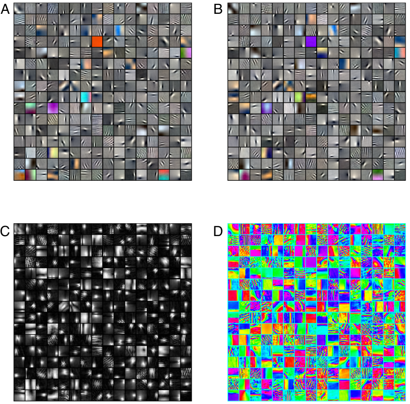
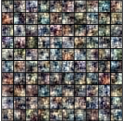
Here we examine the structure represented in the model parameters $R$, $Q$, $P$, and $C$ after training the mpkRBM on natural images. The subspace filters in the $C$ learn localized oriented band-pass filters roughly in quadrature, see Fig. 2. We have observed that the filters in the matrix $C$ appear to learn more textured patterns than those in the mcRBM, but a more rigorous analysis is needed to verify such an observation. The weights in the matrix $P$ adapt to group subspaces with similar spatial position and spatial frequency. See Fig. 4 for a depiction of the image filters with the highest weights to each hidden unit $h^{p}$. The values in the learned matrix $W$ are similar to those learned by the mcRBM and are shown in Fig. 3.

Figure 4: Learned $L_{p}$ groupings, $P$: A random selection (out of 256) columns in $P$. Each column depicts the top 6 weighted subspaces in $C$ for a specific column in $P$. Each subspace in $C$ is two-dimensional and we show the unwhitened image domain weights for both subspaces in A) and B). The corresponding image domain amplitudes and phases for the subspaces are shown in C) and D). There is clear grouping of subspaces with similar positions, orientations, and scales.

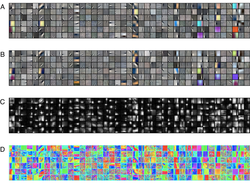
The learned $R$ and $Q$ weights are harder to visualize as they express dependencies in a layer removed from the image domain. However, we can view the subspaces that are weighted highest by each column of $Q$. For each column in Fig. 5 we depict the image domain filters ($C$) that are weighted highest by the corresponding column in $Q$. We similarly show the image domain filters that are weighted highest by each column in $R$ in Fig. 6.

Figure 5: Learned Phase Projections, $Q$: The first 32 (out of 256) columns in $Q$ are shown. The entries in each column of $Q$ weight the cosine or sine of each subspace. Because the cosine and sine correspond to specific vectors in the tensor $C$, we show the image domain projection of these vectors that take the highest weight in the column of $Q$. In this figure, the 6 image domain projections with the highest magnitude weights are shown in the rows for different columns of $Q$ (each is shown in a different column of the figure).

Figure 6: Learned Phase Coupling, $R$: The first 32 (out of 256) columns in $R$. Each column in $R$ produces a different coupling matrix (see Eq. 10). The values in this matrix indicate phase coupling between pairs of subspaces. Therefore, for the matrix $K$ produced by a specific column of $R$, we find the couplings with the highest magnitude. Given these sorted pairs, we take the unique top 6 entries. Finally, we plot the image domain filters corresponding to these 6 entries (shown in the rows). As in Fig. 5 these entries can be mapped to vectors in the tensor $C$ and thus plotted in the image domain. Different columns of $R$ are shown in different columns of the figure.

5 Discussion

The mpRBM and mpkRBM suggest a number of interesting future directions. For example, it should be possible to learn the dimensionality of the subspaces by introducing a weighting matrix in the $L$ dimensional space of the tensor $C$. However, it is not clear how to define an appropriate angle within these subspaces for the phase-coupling factors. Although, it would be reasonable to learn a separate set of factors, $C$, for the $h^{p}$ units and the $h^{k}$ units, thus freeing the constraint of $L=2$ for the $h^{p}$ units. It may also be possible to extend the mpRBM to a nested form of $L_{p}$ distributions suggested in [14]. It is also worth exploring the behavior of the phase-coupling hidden units as the number of hidden units is varied. As we had little prior expectation as to the structure of the learned $R$ and $Q$ matrices, the choice of 100 $h^{k}$ hidden units was rather arbitrary.

6 Conclusions

In this paper we have introduced two new factorized Boltzmann machines: the mpRBM and the mpkRBM, which each extend the factorized third-order Boltzmann machine (the mcRBM) of Ranzato and Hinton [1]. The form of these additional hidden unit factors are motivated by image models of subspace structure [6] and phase alignments due to edges in natural images [8]. Focusing on the mpkRBM, we have shown that such a model learns phase structure in natural images.

7 Acknowledgments

We would like to thank Marc’Aurelio Ranzato for helpful comments and discussions. We would also like to thank Bruno A. Olshausen for his contributions to early drafts of this document. This work has been supported by NSF grant IIS-0917342 (KK) and NSF grant IIS-0705939 to Bruno A. Olshausen.

References

- [1] M. Ranzato and G. Hinton. Modeling pixel means and covariances using factorized third-order boltzmann machines. In Proc. of Computer Vision and Pattern Recognition Conference (CVPR 2010). 2010.
- [2] Y. Karklin and M.S. Lewicki. Emergence of complex cell properties by learning to generalize in natural scenes. Nature, 457(7225):83–86, 2008.
- [3] S. Lyu and E.P. Simoncelli. Modeling multiscale subbands of photographic images with fields of Gaussian scale mixtures. IEEE Trans. Patt. Analysis and Machine Intelligence, 31(4):693–706, April 2009.
- [4] S. Lyu and E.P. Simoncelli. Nonlinear Extraction of Independent Components of Natural Images Using Radial Gaussianization. Neural Computation, 21(6):1485–1519, 2009.
- [5] F. Sinz and M. Bethge. The Conjoint Effect of Divisive Normalization and Orientation Selectivity on Redundancy Reduction in Natural Images. In Frontiers in Computational Neuroscience. Conference Abstract: Bernstein Symposium 2008, 2008.
- [6] U. Koster and A. Hyvarinen. A two-layer ICA-like model estimated by score matching. Lecture Notes in Computer Science, 4669:798, 2007.
- [7] C. F. Cadieu and B. A. Olshausen. Learning transformational invariants from natural movies. In D. Koller, D. Schuurmans, Y. Bengio, and L. Bottou, editors, Advances in Neural Information Processing Systems 21, pages 209–216. MIT Press, 2009.
- [8] P. Kovesi. Phase congruency: A low-level image invariant. In Psychological Research Psychologische Forschung, volume 64, pages 136–148. Springer-Verlag., 2000.
- [9] C. F. Cadieu and K. Koepsell. Phase coupling estimation from multivariate phase statistics. Neural Computation, 22(12):3107–3126, 2010.
- [10] Y. Karklin and M.S. Lewicki. A hierarchical bayesian model for learning nonlinear statistical regularities in nonstationary natural signals. Neural Computation, 17(2):397–423, 2005.
- [11] O. Schwartz and E.P. Simoncelli. Natural signal statistics and sensory gain control. Nature neuroscience, 4(8):819–825, 2001.
- [12] C. Zetzsche, G. Krieger, and B. Wegmann. The atoms of vision: Cartesian or polar? Journal of the Optical Society of America A, 16(7):1554–1565, 1999.
- [13] G.E. Hinton. Training products of experts by minimizing contrastive divergence. Neural Computation, 14(8):1771–1800, 2002.
- [14] F. Sinz, E. P. Simoncelli, and M. Bethge. Hierarchical modeling of local image features through lp-nested symmetric distributions. In Adv. Neural Information Processing Systems 22, volume 22, pages 1696–1704. May 2010.
- [15] G. E. Hinton, S. Osindero, M. Welling, and Y. Teh. Unsupervised discovery of non-linear structure using contrastive backpropagation. Cognitive Science, 30(4):725–731, 2006.
- [16] R.M. Neal. Probabilistic inference using markov chain monte carlo methods. Technical Report CRG-TR-93-1, Dept. of Computer Science, University of Toronto, 1993.