Heat transport in an open transverse-field Ising chain

Abstract

The heat conduction in an open transverse-field Ising chain is studied by using quantization in the Fock space of operators in the weak coupling regimes, i.e. the coupling is much smaller than the transverse field. The non-equilibrium steady state is obtained for large size systems coupled to Markovian baths at its ends. The ballistic transport is observed in the uniform chain and normal diffusion in the random-exchange chain. In addition, the ballistic-diffusive transition is found at the intermediate disorder regime. The thermal conductivity $\kappa$ is also calculated in the low and high temperature regimes. It is shown that $\kappa$ decays as $\kappa\sim T^{-2}$ at high temperatures.

1 Introduction

Heat and spin transport behaviors of one-dimensional systems have intensively been studied in both classical and quantum mechanical context for several decades[1, 2, 3, 4, 5, 6, 7, 8, 9, 10, 11, 12, 13]. Some classical nonlinear systems of interacting particles usually show a diffusive behavior, which satisfy Fourier’s law, $J=-\kappa\nabla T$ ($\kappa$ is the thermal conductivity), relating the macroscopic heat flux to the temperature gradient[14, 15, 16]. In the quantum regime, it is also an important issue that how normal energy or heat is transported through a sample on a microscopic level. The ballistic behavior has been proposed in the integrable quantum systems, implying that the current-current correlation functions typically do not decay to zero[7]. The chaotic dynamics of a nonintegrable system may yield a normal diffusion. One natural question is how the heat transports through a quantum disordered system.

There exists two general theoretical approaches for a description of non-equilibrium open quantum spin systems. One is the non-equilibrium green’s function method[17, 18]. The other is the quantum master equation [19, 20]. In the latter case, various approximations schemes are employed, such as Markov approximations, Born approximations, secular approximations, and weak coupling approximations for the system-environment coupling. Some effective dissipative equations of motion for reduced density matrix $\hat{\rho_{s}}$ of the open systems are then derived.

By using the proper quantum master equation, some interesting and important thermal properties have been found in the open spin-chain systems by using the Monte Carlo wave function method[5, 21, 22, 23], the matrix product operator method[24], and fourth order Runge-Kutta method[1, 3, 4]. However, the largest system sizes reported in the literature is smaller than $N=20$, and the convincing results for the properties and the type of the transport are still lacking to date. In the meantime, some progresses in the methodology have also been achieved, such as the adaptive time-dependent density matrix renormalization group, the numerically exact diagonalization and the quantization in the Fock space of operators etc.[25, 26, 27, 28, 29], which could be applied in the large system successfully. Therefore, the studies on the large size system have become an essential and intensive issues. Recently, Prosenet al.[29] proposed a method to solve explicitly the Lindblad master equation for an arbitrary quadratic system of $n$ fermions in terms of diagonalization of a $4n\times 4n$ matrix. This method has been successfully applied to the far from equilibrium quantum phase transition[30, 31] in one-dimensional XY spin chain for size larger than $100$.

In this paper, we study the heat current properties of the well known 1D transverse field Ising model with very large sizes. The exchange couplings are considered to be both uniform and random. The decisive conditions of the ballistic transport and the normal transport are given. The paper is organized as follows: In Sec.II, we describe the model and the scheme to solve the quantum master equation in detail. Then the numerical results are obtained in Sec.III. The conclusion is given in the last section.

2 MODEL AND METHOD

The Hamiltonian for an open 1D transverse field Ising chain reads

$$H = -\sum_{n=1}^{N}h\sigma_{n}^{z}-\sum_{n=1}^{N-1}J_{n}\sigma_{n}^{x}\sigma_{n+1}^{x},$$ (1)

where $N$ is the number of spins, the operators $\sigma_{n}^{x}$ and $\sigma_{n}^{z}$ are the Pauli matrices for the $n$th spin, $J_{n}$ is the coupling parameter between the nearest-neighbor spins, and $h$ is the transverse magnetic field. Here we take $h=1$. For the disordered system, $J_{n}$ is chosen to distribute on a interval $(0.05,0.15)$ uniformly, modeling the weak coupling condition. For the uniform system, we take $J_{n}=0.15$. Considering the two thermal baths at two ends and the coupling with the Ising chain, the total Hamiltonian can be written as

$$\mathcal{H} = H+H_{L}+H_{R}+H_{int},$$ (2)

where $H_{L(R)}=\sum_{k}^{L(R)}\hbar\omega_{k}a_{k}^{\dagger}a_{k}$ is the left(right) phonon bath with $a_{k}^{\dagger}$($a_{k}$) the phonon creation(annihilation) operator, and $H_{int}=\sigma_{1(N)}^{\mp}\sum_{k}^{L(R)}(g_{k}a_{k}+g_{k}^{*}a_{k}^{\dagger})$ is the interaction between the chain and the baths. If the coupling $g_{k}$ is weak, a quantum master equation for the system s evolution can be obtained from our microscopic Hamiltonian model by using the usual Born-Markov approximations and the secular approximation[19].

The quantum master equation in the weak internal coupling limit($\{J_{n}\}\ll h$) reads (we set $\hbar=1$)

$$\frac{d\rho}{dt}=-i[H,\rho]+D_{L}(\rho)+D_{R}(\rho),$$ (3)

where the dissipator $D_{L}$ refers to the left heat bath and $D_{R}$ to the right one, depending on the full density operator $\rho$ of the Hamiltonian (1). Eq. (3) can be rewritten as the Lindblad master equation

$$\frac{d{\rho}}{dt}=\mathcal{\hat{L}}\rho:=-i[H,\rho]+\sum_{\mu}(2L_{\mu}\rho L_{\mu}^{\dagger}-\{L_{\mu}^{\dagger}L_{\mu},\rho\}),$$ (4)

where $L_{\mu}$s are the Lindblad operators, representing couplings to different baths. The weak bath coupling is taken into account here. The simplest nontrivial bath operators acting only on the first and the last spin are chosen ($\mu=1,2,3$, and $4$)

$$L_{1,2}=\sqrt{\Gamma_{1,2}^{L}}\sigma_{1}^{\mp},\quad L_{3,4}=\sqrt{\Gamma_{1,2}^{R}}\sigma_{N}^{\mp},$$ (5)

where $\sigma_{m}^{\mp}=(\sigma_{m}^{x}\pm i\sigma_{m}^{y})/2$. Refer to Refs. [2, 29, 30], we have $\Gamma_{1}^{L,R}=\pi\lambda_{B}[1+n_{L,R}(\omega)]I(\omega)|_{\omega=2h}\equiv\lambda[1+n_{L,R}(2h)]$ and $\Gamma_{2}^{L,R}=\pi\lambda_{B}n_{L,R}(\omega)I(\omega)|_{\omega=2h}\equiv\lambda n_{L,R}(2h)$. Here, $n_{L,R}(\omega)=(e^{\omega/T_{L,R}}-1)^{-1}$ is the Bose-Einstein distribution function ($k_{B}=1$), $\lambda_{B}$ is the system-bath coupling strength, and $I({\omega})$ denotes the spectral density of an Ohmic bath that we choose. The Hamiltonian (1) is conveniently expressed as a quadratic form $H=\underline{w}\cdot\textbf{H}\underline{w}$ in terms of $2N$ Hermitian Majorana operators

$$w_{2n-1}=\sigma_{n}^{x}\prod_{n^{\prime}<n}\sigma_{n^{\prime}}^{z},\quad w_{2n}=\sigma_{n}^{y}\prod_{n^{\prime}<n}\sigma_{n^{\prime}}^{z},$$ (6)

satisfying the anticommutation relation $\{w_{n},w_{m}\}=2\delta_{n,m}$. H is an $2N\times 2N$ antisymmetry Hermite matrix ($\textbf{H}^{T}=-\textbf{H}$). Based on the previous transformation, we can rewrite Hamiltonian (1) in terms of Majorana fermions

$$H = i\sum_{n=1}^{N}hw_{2n-1}w_{2n}+i\sum_{n=1}^{N-1}J_{n}w_{2n}w_{2n+1},$$ (7)

$$L_{1,2}=\sqrt{\Gamma_{1,2}^{L}}(w_{1}\mp iw_{2}),$$

$$L_{3,4}=-(-i)^{N}\sqrt{\Gamma_{1,2}^{R}}(w_{2N-1}\mp iw_{2N})W,$$ (8)

where $W=w_{1}w_{2}\cdots w_{2N}$ is a Casimir operator which commutes with all the elements of the Clifford algebra generated by $w_{j}$[29]. Note that $W^{2}=1$, so it does not affect the quadratical system. For convenience, we take $W=1$.

Then we construct $4^{N}$ dimensional Pauli algebra with a Fock space of operators describing $2N$ adjoint fermions (a-fermions), with an orthonormal canonical basis $|P_{\underline{\alpha}}\rangle=|w_{1}^{\alpha_{1}}w_{2}^{\alpha_{2}}\cdots w_{2N}^{\alpha_{2N}}\rangle$, $\alpha_{j}\in\{0,1\}$. With the definition $\hat{c}_{j}|P_{\underline{\alpha}}\rangle=\delta_{\alpha_{j,1}}|w_{j}P_{\underline{\alpha}}\rangle$, the quantum Liouvillean (4) becomes bilinear $\mathcal{\hat{L}}=\underline{\hat{a}}\cdot\textbf{A}\underline{\hat{a}}+const\bf 1$ in Hermitian maps $\hat{a}_{2j-1}=\frac{1}{\sqrt{2}}(\hat{c}_{j}+\hat{c}_{j}^{\dagger})$, $\hat{a}_{2j}=\frac{1}{\sqrt{2}}(\hat{c}_{j}-\hat{c}_{j}^{\dagger})$, obeying $\{\hat{a}_{p},\hat{a}_{q}\}=\delta_{p,q}$. The $4N\times 4N$ matrix A can be expressed in a block tridiagonal form in terms of $4\times 4$ matrices as

$$\textbf{A}=\left(\begin{array}[]{ c c c c l r }\textbf{B}_{L}-2h\textbf{R}&\textbf{R}_{1}&\textbf{0}&\dots&\textbf{0}\\ -\textbf{R}_{1}^{T}&-2h\textbf{R}&\textbf{R}_{2}&\ddots&\textbf{0}\\ \textbf{0}&-\textbf{R}_{2}^{T}&-2h\textbf{R}&&\vdots\\ \vdots&\ddots&&\ddots&\textbf{R}_{N-1}\\ \textbf{0}&\textbf{0}&\dots&-\textbf{R}_{N-1}^{T}&\textbf{B}_{R}-2h\textbf{R}\end{array}\right),$$ (9)

where

$$\textbf{B}_{L,R}=\left(\begin{array}[]{ c c c c l r }0&2i\Gamma_{+}^{L,R}&-2i\Gamma_{-}^{L,R}&2\Gamma_{-}^{L,R}\\ -2i\Gamma_{+}^{L,R}&0&2\Gamma_{-}^{L,R}&2i\Gamma_{-}^{L,R}\\ 2i\Gamma_{-}^{L,R}&-2\Gamma_{-}^{L,R}&0&2i\Gamma_{+}^{L,R}\\ -2\Gamma_{-}^{L,R}&-2i\Gamma_{-}^{L,R}&-2i\Gamma_{+}^{L,R}&0\end{array}\right)$$ (10)

with $\Gamma_{\pm}^{L,R}=\Gamma_{2}^{L,R}\pm\Gamma_{1}^{L,R}$ and

$$\textbf{R}=\left(\begin{array}[]{ c c c c l r }0&0&-1&0\\ 0&0&0&-1\\ 1&0&0&0\\ 0&1&0&0\end{array}\right),\textbf{R}_{m}=\left(\begin{array}[]{ c c c c l r }0&0&0&0\\ 0&0&0&0\\ 2J_{m}&0&0&0\\ 0&2J_{m}&0&0\end{array}\right).$$ (11)

The eigenvalues of $4N\times 4N$ antisymmetric A called rapidities can be list in the form of the pairs $\beta_{1},-\beta_{1},\beta_{2},-\beta_{2},\dots,\beta_{2N},-\beta_{2N}$, Re$\beta_{j}\geq 0$. The corresponding eigenvectors $\underline{v}_{p}$ ( $p=1,\dots,4N$ ) can be defined by $\textbf{A}\underline{v}_{2j-1}=\beta_{j}\underline{v}_{2j-1}$ and $\textbf{A}\underline{v}_{2j}=-\beta_{j}\underline{v}_{2j}$. $\underline{v}$ can be normalized by using $\underline{v}_{2j-1}\cdot\underline{v}_{2j}=1$ and $\underline{v}_{p}\cdot\underline{v}_{q}=0$ otherwise, which can be used to calculate any quadratic physical observable in the non-equilibrium steady state (NESS). The expectation value is given by

$$\langle w_{j}w_{k}\rangle_{NESS} = \delta_{j,k}+\frac{1}{2}\sum_{n=1}^{2N}(v_{2n,2j-1}-iv_{2n,2j})$$ (12)

$$\times(v_{2n-1,2k-1}-iv_{2n-1,2k}).$$

3 NUMERICAL RESULTS

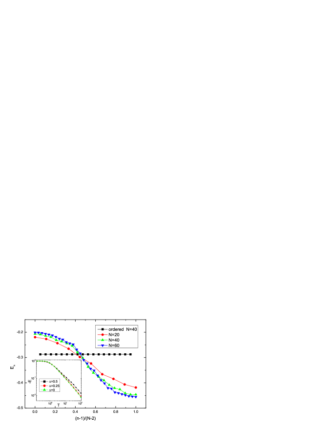
Figure 1: (color online) Energy profiles $E_{n}$ (odd sites) for a random chain with different sizes $N$. $J_{n}\in(0.05,0.15)$, $T_{L}=5$, $T_{R}=2$. For comparison, the energy profile $E_{n}$ of an ordered chain with $J_{n}=J=0.1$ is also listed. The inset denotes the local energy $E_{2}$ versus average temperature $T$ for the disordered system ($N=4$) with different temperature difference $\Delta$. All results are averaged over 200 realizations of disorder.

First, to show the correctness of this method, we numerically calculate the local energy $E_{n}$. The local energy density operator reads

$$H_{n}=iJ_{n}w_{2n}w_{2n+1}+i\frac{h}{2}(w_{2n-1}w_{2n}+w_{2n+1}w_{2n+2}),$$ (13)

and local energy density is defined as $E_{n}=\langle H_{n}\rangle_{NESS}$. The temperatures of the left and right baths are $T_{L}=T(1+\Delta)$ and $T_{R}=T(1-\Delta)$, where $\Delta$ is the dimensionless temperature difference and $T$ is the average temperature. We set the coupling constants uniformly distribute on the interval $J_{n}\in(0.05,0.15)$, which are the same as those in Ref. [1]. $\lambda$ is taken as 0.005, which is equivalent to the parameter $\alpha=0.01$ in the Ref. [1]. The numerical results for local energy $E_{n}$ with different sizes are presented in Fig. 1. Here we only plot the local energy on the odd sites for the similar results on the even sites. Note that there is a clear intersection of the energy profiles $E_{n}$ (disordered) for different sizes at the central part of the chain. And the inset shows $E_{2}$ versus $T$ for $N=4$. The local energy decreases with the increase of $\Delta$. When $\Delta=0$, the results can be checked with the canonical one[1]. It is interesting that the present local energy is nearly the same as those in Ref. [1]. It should be pointed out here that the method is not suited to the strong coupling case, since the Lindblad equation is only valid for small $\{J_{n}\}$.

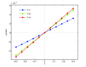
Figure 2: (color online) Heat current vs temperature difference for the uniform system. The average temperature $T$ changes from 1 to 3. The other parameters are $h=1$, $J_{n}=0.15$, $\lambda=0.005$, and $N=100$.

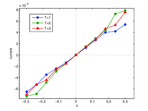
Figure 3: (color online) Heat current vs temperature difference for the disordered system. The range of $T$ is set from 1 to 3. The other parameters are $h=1$, $J_{n}\in(0.05,0.15)$, $\lambda=0.005$, and $N=100$. The results are averaged over 100 realizations of disorder.

Then we evaluate the heat current in the spin chain in NESS

$$Q_{n} = i[H_{n},H_{n+1}]$$ (14)

$$= i[-J_{n}hw_{2n}w_{2n+2}-hJ_{n+1}w_{2n+1}w_{2n+3}].$$

The heat current as a function of the temperature difference for $N=100$ chain is presented in Fig. 2 for the uniform case and Fig. 3 for the disordered case with the mean temperature ranging from $T=1$ to $3$. According to Eq. (5), the high bath temperature can enhance the coupling strength between the baths and the spin chain, which facilitates the heat transfer. So $\kappa$ increases with the augmentation of the average temperature $T$ in the given parameters regime, as shown in Fig. 2. For the disordered case, $\kappa$ changes little in small $\Delta$ regimes ($-0.1<\Delta<0.1$), as shown in Fig. 3. From the order of magnitude of the heat current, one can see that the current is easily blocked for the disordered case.

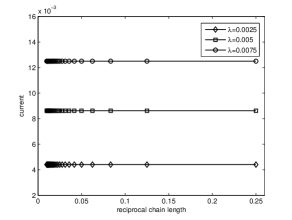
Figure 4: Heat current versus reciprocal chain length for different bath coupling strength $\lambda$ for the uniform system. The parameters are $J_{n}=0.15$, $h=1$, $\beta_{L}=1/T_{L}=0.25$ and $\beta_{R}=1/T_{R}=0.75$.

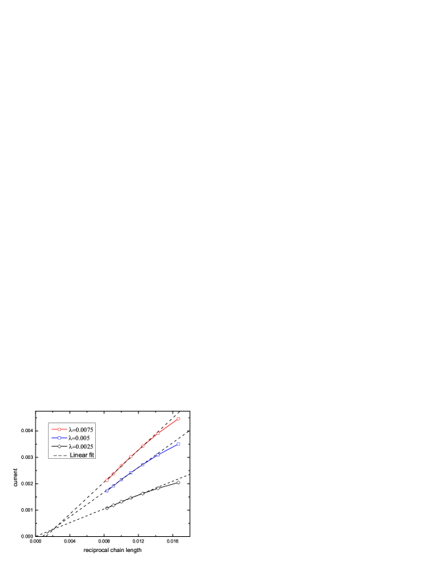
Figure 5: (color online) Heat current versus reciprocal chain length for the disordered system. System parameters: $J_{n}\in(0.05,0.15)$, $h=1$, $\beta_{L}=1/T_{L}=0.25$ and $\beta_{R}=1/T_{R}=0.75$ . The sizes of the system range from $60$ to $120$ every other $10$ sites. The results are averaged over $2000$ realizations of disorder.

We turn to discuss the classification of heat transport properties. Note that a finite current within an infinite system demonstrates ballistic transport behavior. In the previous studies, the ballistic behavior is observed in the integrable system, and the diffusive transport occurs for the disordered system. But these conclusions were built on the numerical simulations on small systems[1, 3, 5, 10, 11].

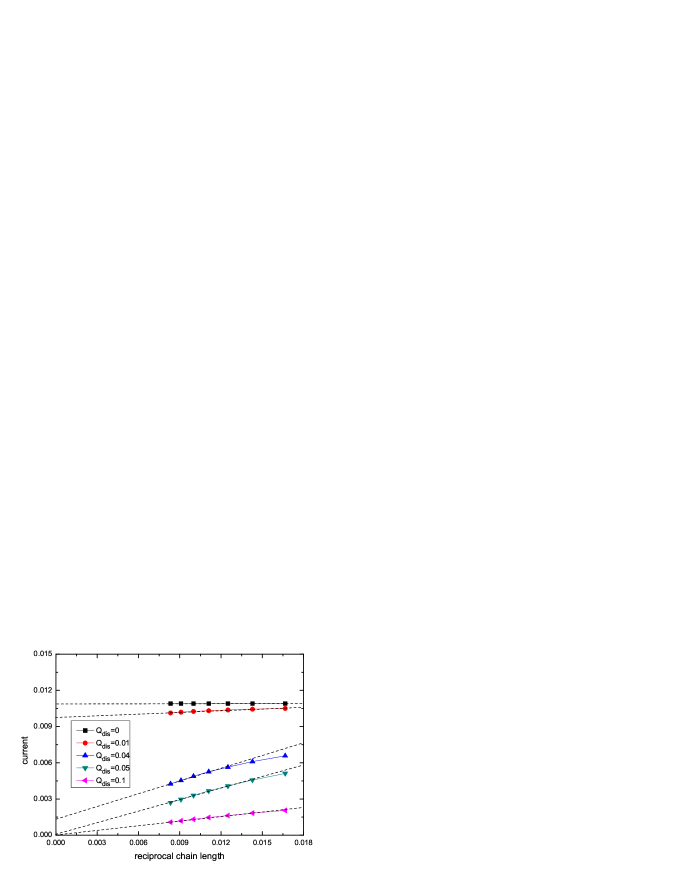
Figure 6: (color online) Heat current versus reciprocal chain length for different disorder strengthes. System parameters are $h=1$, $\lambda=0.0025$, $\beta_{L}=1/T_{L}=0.25$, and $\beta_{R}=1/T_{R}=0.75$. The results are averaged over $2000$ realizations of disorder.

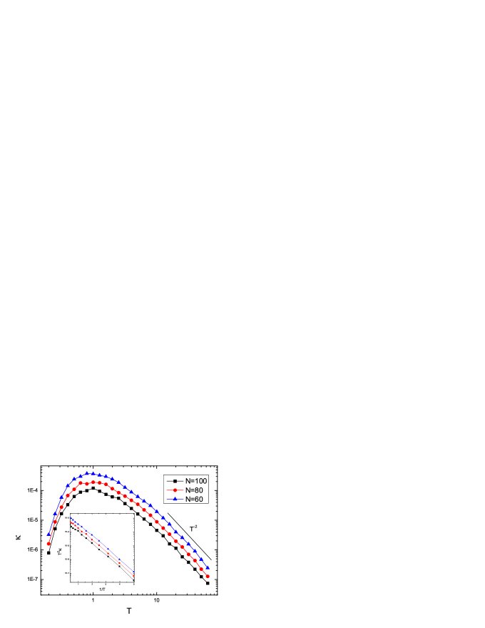
Figure 7: Thermal conductivity $\kappa$ versus $T$ for the disordered system with $J_{n}\in(0.05,0.15)$, $h=1$ and different sizes $N=60,80,100$. The bath temperatures are $T_{L}=T(1+\Delta)$ and $T_{R}=T(1-\Delta)$ ($\Delta=0.02$). The results are averaged over $200$ realizations of disorder. The inset shows the low temperature property of thermal conductivity.

To classify transport properties more convincingly, we simulate the system with the size up to $N>100$ for both cases. The numerical results are plotted in Figs. 4 and 5. Note that the ballistic transport occurs at the uniform case, as shown in Fig. 4. The heat current increases with the bath coupling strength $\lambda$. Different from the observation in a Heisenberg chain[5], the present heat current is only sensitive to the parameter $\lambda$ and independent of the system size, which is just the characteristics of the ballistic transport only emerging in a quantum system. The known Fourier’s law is obviously invalid. For the disordered case, the current is gradually reduced with increasing the system size, demonstrating the diffusive transport, as exhibited in Fig. 5. The similar results are also obtained in the mass-disordered harmonic crystals[32]. For the present system size $N=100$, $1/N$ scaling behavior of the heat current is observed for $\lambda=0.0025$, demonstrating that the Fourier’s law holds in this case. So we provide an evidence of the macroscopic heat transport in the quantum disordered system. With the increase of the coupling parameter $\lambda$, the linear fit gradually deviates from the origin of the coordinate, implying that the finite-size effect is more obvious for large coupling parameters, thus the data for large systems would be essential to get the correct scaling for strong coupling.

At this stage, it should be expected that the ballistic-diffusive transition might occur at the intermediate disorder regime. The disorder strength is introduced in the coupling parameter $J_{n}=0.1+Q_{dis}\varepsilon$, where $\varepsilon$ distributes uniformly on the interval $(-0.5,0.5)$. We plot the heat current vs reciprocal chain length for different disorder strengthes in Fig. 6. The linear fit of the data shows that the transition occurs at $Q_{dis}=0.04\sim 0.05$.

Finally, we obtain the fully thermal conductivity $\kappa$ as a function of temperature in the different large sizes for the disordered case. In the high temperature regime, it is observed that $\kappa$ decays slightly faster than $T^{-2}$, as shown in Fig. 7. $\kappa$ reaches a maximum value around $T=1.0$ with different sizes $N$. The thermal conductivity decreases with increasing system size. The inset presents the relation $ln(T^{2}\kappa)\propto 1/T$ in the low temperature regime. The thermal conductivity $\kappa$ and the specific heat $c_{v}$ of a single spin have a similar temperature dependence. These observations are consistent with the analytic and numerical results of Ref. 1 based on a smaller system.

4 Conclusions

In this paper, we have studied the heat transport behaviors of an open Ising chain within master equation formalism by using quantization in the Fock space of operators. The classification of the transport properties is performed in large size system (over $100$ sites). Compared with the Monte Carlo wave-function method, the precision has been considerably improved in the present approach. We confirm the ballistic current in the uniform system which is integrable. The normal transport is clearly observed in the disordered system. The bulk conductivity decreases with the increase of the system size. The heat current exhibits a diffusive behavior above a critical interaction strength, which follows Fourier’s law in the normal transport. Moreover, the ballistic-diffusive transition occurs at the intermediate disorder regime. It is also observed that the thermal conductivity $\kappa$ has the similar temperature dependence as the specific heat $c_{v}$ in the weak coupling regime.

- [1] Y. H. Yan, C. Q. Wu, G. Casati, T. Prosen, and B. W. Li, Phys. Rev. B 77, (2008) 172411.
- [2] C. Mejia-Monasterio and H. Wichterich, Eur. Phys. J. Special Topics 151, PP. 113-125 (2007).
- [3] Y. H. Yan, C. Q. Wu, and B. W. Li, Phys. Rev. B 79, (2009) 014207.
- [4] L. F. Zhang, Y. H. Yan, C. Q. Wu, J. S. Wang, and B. W. Li, Phys. Rev. B 80, (2009) 172301.
- [5] M. Michel and O. Hess, Phys. Rev. B 77, (2008) 104303.
- [6] X. Zotos, F. Naef, and P. Prelovk, Phys. Rev. B 55, (1997) 11029.
- [7] A. V. Sologubenko, E. Felder, K. Giann, H. R. Ott, A. Vietkine, and A. Revcolevschi, Phys. Rev. B 62, (2000) R6108; A. V. Sologubenko, K. Giann, H. R. Ott, A. Vietkine, and A. Revcolevschi, ibid. 64, (2001) 054412.
- [8] K. Saito, Europhys. Lett. 61, (2003) 34.
- [9] C. Mejia-Monasterio, T. Prosen, and G. Casati, Europhys. Lett. 72, (2005) 520.
- [10] M. Michel, M. Hartmann, J. Gemmer, and G. Mahler, Eur. Phys. J. B 34, (2003) 325.
- [11] M. Michel, G. Mahler, and J. Gemmer, Phys. Rev. Lett. 95, (2005) 180602.
- [12] R. Steinigeweg, J. Gemmer, and M. Michel, Europhys. Lett. 75, (2006) 406.
- [13] P. Jung, R. W. Helmes, and A. Rosch, Phys. Rev. Lett. 96, (2006) 067202.
- [14] B. Hu, B. Li, and H. Zhao, Phys. Rev. E 57, (1998) 2992; B. Hu, B. Li, and H. Zhao, ibid. 61, (2000) 3828; K. Aoki and D. Kusnezov, Phys. Lett. A 265, (2000) 250.
- [15] R. E. Peierls, Quantum Theory of Solids (Oxford University Press, London, 1955).
- [16] K. Saito and A. Dhar, Phys. Rev. Lett. 104, (2010) 040601.
- [17] R. Kubo, J. Phys. Soc. Jpn. 12, (1957) 570.
- [18] H. Mori, Phys. Rev. 115, (1959) 298.
- [19] S. Kryszewski and J. Czechowska-Kryszk, arXiv:quant-ph/0801.1757v1 (2008).
- [20] H. Wichterich, M. J. Henrich, H. P. Breuer, J. Gemmer, and M. Michel, Phys. Rev. E 76, (2007) 031115.
- [21] G. G. Carlo, G. Benenti, and G. Casati, Phys. Rev. Lett. 91, (2003) 257903.
- [22] G. Lindblad, Commun. Math. Phys. 48, (1976) 119.
- [23] H.-P. Breuer and F. Petruccione, The theory of open quantum systems, (Oxford University Press, London, 2002).
- [24] T. Prosen and Marko nidari, J. Stat. Mech. (2009) P02035.
- [25] Y. Dubi and M. D. Ventra, Phys. Rev. B 79, (2009) 115415.
- [26] S. Langer, F. Heidrich-Meisner, J. Gemmer, I. P. McCulloch, and U. Schollwöck, Phys. Rev. B 79, (2009) 214409.
- [27] R. Steinigeweg and J. Gemmer, Phys. Rev. B 80, (2009) 184402.
- [28] D. Karevski and T. Platini, Phys. Rev. Lett. 102, (2009) 207207.
- [29] T. Prosen, New J. Phys. 10, (2008) 043026.
- [30] T. Prosen and I. Piorn, Phys. Rev. Lett. 101, (2008) 105701.
- [31] I. Piorn and T. Prosen, Phys. Rev. B 79, (2009) 184416.
- [32] A. Chaudhuri, A. Kundu, D. Roy, A. Dhar, J. L. Lebowitz, and H. Spohn, Phys. Rev. B 81, (2010) 064301.