Data characterization using artificial-star tests: performance evaluation

Abstract

Traditional artificial-star tests are widely applied to photometry in crowded stellar fields. However, to obtain reliable binary fractions (and their uncertainties) of remote, dense, and rich star clusters, one needs to recover huge numbers of artificial stars. Hence, this will consume much computation time for data reduction of the images to which the artificial stars must be added. In this paper, we present a new method applicable to data sets characterized by stable, well-defined point-spread functions, in which we add artificial stars to the retrieved-data catalog instead of the raw images. Taking the young Large Magellanic Cloud cluster NGC 1818 as an example, we compare results from both methods and show that they are equivalent, while our new method saves significant computational time.

1 Introduction

The artificial-star-test technique has been widely applied to photometry of crowded stellar fields over the last few decades. By adding artificial stars to the original, raw images and subsequently recovering them, such tests have proved an efficient means of counting stars as a function of magnitude and measuring the associated photometric accuracies (e.g., Bolte 1989, 1994; Bergbusch 1996; Sandquist et al. 1996; Da Rocha et al. 2002; Hargis et al. 2004; Fekadu et al. 2007). Modern computers (‘central processing units:’ CPUs) are becoming ever more powerful, thus providing opportunities to perform artificial-star experiments to characterize the color-magnitude-diagram (CMD) morphologies of remote, rich star clusters and obtain cluster binary fractions by comparing CMDs based on artificial and real stars (e.g., Rubenstein & Bailyn 1997; Zhao & Bailyn 2005; Hu et al. 2010).

However, even with the current generation of CPUs, this method still consumes significant computation time if one wants to use it to derive cluster binary fractions, for which many more (artificial) stars are needed than to obtain observational completeness levels. For instance, Bolte (1994) used $5.5\times 10^{4}$ artificial stars (in 450 test runs, i.e., on the order of 100 stars per trial, which must be compared to 200 artificial stars per run used in this paper; see below) to calculate the completeness fraction of his observations of the globular cluster M30, where they recovered 5674 real stars within the range $13\leq V\leq 22$ mag. Similarly, Bellazzini et al. (2002) required $1.5\times 10^{6}$ artificial stars ($17\leq V\leq 25$ mag) to obtain an estimate of the binary fraction in NGC 288 (compared with 5766 observed stars in the cluster’s central regions and 2013 near its half-light radius, with $13\leq V\leq 25.5$ mag).

With such large artificial-star catalogs, both the addition of stars to the images and the subsequent data reduction required for recovery of these artificial stars will be enormously time-consuming. As an altenative, Hu et al. (2010) developed and applied a novel, efficient method (in which they added artificial stars to the catalog instead of the images) to obtain the binary fraction of the young Large Magellanic Cloud cluster NGC 1818.

In this paper, we use the raw images of NGC 1818, taken with the Wide Field and Planetary Camera-2 (WFPC2) on board the Hubble Space Telescope (HST) as an example to benchmark and compare the performance of both artificial-star-test methods. The photometric data are discussed in §2. The commonly used method of adding artificial stars to images and our newly developed method to correct for stellar blends and superpositions based on catalog handling are presented in §3. A detailed comparison of the two methods and validation of our new approach are provided in §4.

2 Data reduction

Our example data set was obtained from HST program GO-7307 (PI Gilmore), which included three images in both the F555W and F814W filters (with exposure times of 800, 800, and 900 s for each filter), centered at the cluster’s half-light radius. The observations were reduced as described in Hu et al. (2010) using HSTPhot (version 1.1, May 2003; Dolphin 2005).

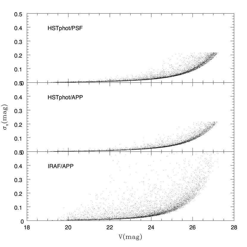
Figure 3: Standard deviations of the photometric uncertainties as a function of stellar magnitude (cf. Hu et al. 2010).

In the left-hand panel of Fig. 1 we show the resulting CMD, reduced using HSTPhot with the point-spread-function (PSF)-fitting option. The corresponding CMDs, reduced using both HSTPhot with the aperture-photometry (‘APP’) option and iraf’s apphot task (Liu et al. 2009), are shown in the middle and right-hand panels. Within the magnitude range from approximately 19 to 27 in both the F555W and F814W filters (an unambiguous detection in both filters was required), we recovered a total of 8756 and 7773 stars using PSF fitting and aperture photometry based on HSTPhot, respectively, while Liu et al. (2009) recovered 7332 stars from the same data set (but for $V\leq 26$ mag). Our new CMDs are much cleaner (we rejected stars with $\chi>1.5$, which is a measure of the signal-to-noise ratio and a level recommended in the HSTphot manual; cf. Dolphin 2000) than that of Liu et al. (2009), who did not apply a cut in signal-to-noise ratio, and the cluster’s main sequence is much tighter. Fig. 3 shows the standard deviations of the photometric uncertainties as a function of stellar magnitude. It is clear that, for the same magnitude range, the uncertainties associated with photometry of stars reduced by HSTPhot are smaller than the equivalent values resulting from application of iraf/apphot. This indicates that our most recently obtained photometry is more precise than that published by Liu et al. (2009), because the HSTphot software package is much better at properly handling stellar photometry in crowded HST fields than iraf’s apphot routine.

Note that although the PSF-fitting approach recovered approximately a thousand more stars than the number detected by aperture photometry, the number of stars brighter than $m_{\rm F555W}=25$ mag (but recall that stars must be detected in both the F555W and F814 filters to be included) was 5974 versus 5791 for the PSF-fitting and aperture-photometry approaches, respectively. The corresponding growth curves for all three reduction methods are shown in Fig. 2 and tabulated in Table 1. The numbers of stars resulting from PSF fitting and aperture photometry are comparable; they are much more numerous than those resulting from the use of iraf/apphot (Liu et al. 2009). Therefore, we conclude that HSTPhot is more appropriate than standard iraf tasks to deal with stellar photometry in crowded HST images and that in crowded fields, such as for NGC 1818, there is no significant difference in performance between the two photometric methods supported by HSTPhot (except for faint stars close to the detection limit; see also §4).

3 Artificial-star tests

We developed our own routines, which we used instead of the iraf/addstar task, to add artificial stars to the images. The masses of the artificial stars were selected from a Salpeter (1955)-like mass function, which was shown to be appropriate for this cluster by de Grijs et al. (2002), Liu et al. (2009), and Hu et al. (2010) for stellar masses in excess of 0.5 to $1M_{\odot}$. For each star, we calculated the magnitude and color by interpolation of the best-fitting Girardi et al. (2000) isochrone for a cluster age of 25 Myr and a metallicity of $Z=0.008$ (where $Z_{\odot}=0.019$). Next, we converted the stellar absolute magnitude in the $V$ band ($M_{V}$) to a total pixel value (PV) using $M_{V}=-2.5\log\mbox{\it PV}+M_{0}$, where $M_{0}$ is the zero-point offset (cf. Hu et al. 2010): $M_{0}=-2.5\log({\rm PHOTFLAM})+{\rm PHOTZPT}$, where PHOTFLAM and PHOTZPT ($=-21.1$) are image-header keywords. Since the CCD’s charge-transfer efficiency (CTE) is a function of position, we used the prescription of Whitmore et al. (1999) to calculate CTE corrections. We calculated scaled HST/WFPC2 PSFs using TinyTim (Krist & Hook 2004) for different filters, positions, and stellar types, before adding appropriately constructed artificial stars to the science images. To do so, we used the TinyTim PSFs to expand the point sources to extended sources ($64\times 64$ pixels² for the Planetary Camera chip, PC1, and $30\times 30$ pixels² for the Wide Field chips, WF1, 2, and 3). The artificial stars were uniformly spread across the images. To avoid interference between artificial stars, we only added 50 stars at any one time to a given chip. In addition, we ensured that each artificial star occupied a unique $64\times 64$ (or, as appropriate, $30\times 30$) pixels² subfield. Finally, we used the same approach (i.e., identical to that used for the analysis of our science data) to recover the added artificial stars from the artificial-star images.

An alternative method to perform artificial-star tests is based on adding stars to the catalog rather than the images (Hu et al. 2010). By applying this method, we do not need to use PSFs to add artificial stars repeatedly to the images and reduce hundreds of thousands of artificial-star images. This will, therefore, potentially save much computation time. Unlike while adding artificial stars to the images, the effects of superposition are automatically included. When we add artificial stars to the spatial-distribution diagram obtained from the catalog, we assume that if an artificial star is located at a distance from any real star of less than 2 pixels (corresponding to the size of our aperture), it is ‘blended.’ In this case, we simply add the fluxes of the artificial and real stars to recalculate the artificial star’s magnitude and color. If the output artificial star is 0.752 mag (or more) brighter than the input value, it is assumed to be blended and rejected from the output artificial-star catalog.

4 Comparison

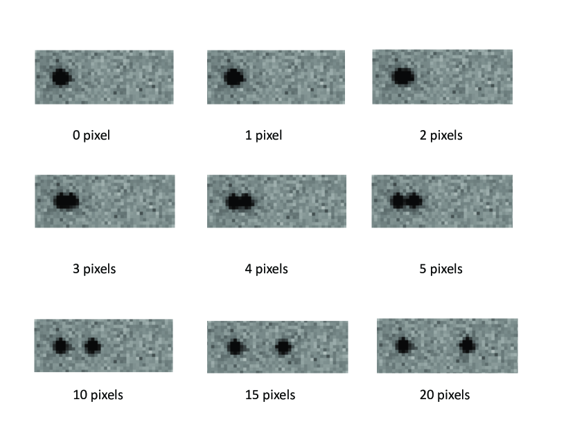
Figure 4: Images of artificial stars added to the raw science frames. The masses of the two stars are both $1.6M_{\odot}$, and the labels refer to the separation between the stars.

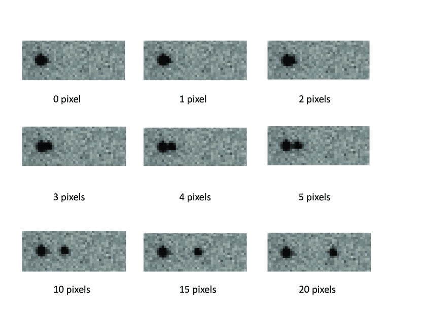
Figure 5: Same as Fig. 4. The masses of the two stars are $1.6$ and $1.3M_{\odot}$.

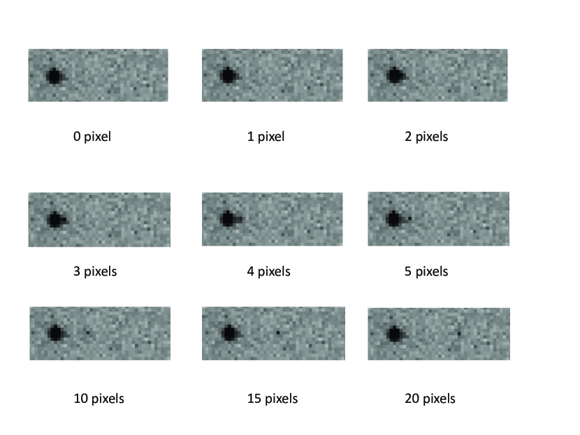
Figure 6: Same as Fig. 4. The masses of the two stars are $1.6$ and $0.8M_{\odot}$.

We performed extensive artificial-star experiments to test the validity of our assumption that stellar images centered within 2 pixels of each other cannot be distinguished individually. To do so, we added sets of two artificial stars to a blank WF2 subfield (i.e., a subfield without any real stars detectable above the noise level, and with realistic noise characteristics). We adopted separations between both stars of $\Delta d=0,1,2,3,4,5,10,15$, and 20 pixels. The resulting images, for a range of stellar-mass ratios, are shown in Figs 4, 5, and 6. We then performed photometry using HSTphot and attempted to recover the fluxes of both stars. Fig. 7 shows the magnitudes of the recovered artificial stars as a function of their separation, assuming input masses of $1.6M_{\odot}$ for both. The recovered magnitude decreases rapidly for separations of less than 2 pixels and reaches a plateau beyond this separation. The difference between the combined flux at $\Delta d=0$ pixel and the recovered magnitudes for the individual artificial stars reaches 0.753 mag at $\Delta d=2$ pixels (in the sense that they are fainter for this $\Delta d$ than when they are blended). This indicates that our assumption of a 2-pixel minimum separation to distinguish two stars individually is a good approximation.

4.1 Completeness

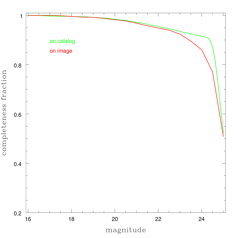
Figure 9: Completeness fractions obtained from the two methods.

We also performed completeness tests. Incompleteness of bright stars is dominated by superpositions in the crowded stellar environment of our observations, while for faint stars it is dominated by the instrument’s detection limit. We adopted a Gaussian-type photometric error for each artificial star (see below), which was added to the spatial-distribution catalog. We also set a 50% completeness limit at $m_{\rm F555W}=25$ mag. If the output artificial star is 0.752 mag (or more) brighter than the input value, the star is blended; if its magnitude is fainter than $m_{\rm F555W}=25$ mag, it cannot be detected. Fig. 9 shows the resulting completeness fraction, calculated by adding 10,000 artificial stars to both the catalog and the images at any one time.

Both incompleteness fractions agree fairly well for stars brighter than $m_{\rm F555W}=23$ mag. Therefore, we conclude that our new method is adequate for studying the binary fractions of stars that are at least $\sim 2$ mag brighter than the observational completeness limit. For fainter stars, our new method cannot be applied with sufficient reliability to estimate completeness fractions. This is so, because by adding artificial stars to the catalog, the completeness fraction will be marginally higher than we would have measured from adding these stars to the images, because we do not take into account the presence of cosmic rays and bad pixels. Therefore, although it offers a quick, first-order indication of a stellar sample’s observational completeness, our method cannot be used to calculate realistic, quantitative incompleteness fractions of real observational data.

4.2 Error analysis

When adding artificial stars to the catalog, we assumed that the photometric errors are distributed in a Gaussian manner. We obtain the relation between stellar magnitude and the corresponding errors from the catalog. We used an exponential function to fit the relation (cf. Hu et al. 2010). To test this assumption, we added 500 artificial stars of the same mass to the raw images and subsequently recovered them using standard data-reduction techniques. Fig. 10 shows the distribution of the differences between the input and output F555W magnitudes (converted to $V$). The mean photometric error is 0.017 mag, while the standard deviation of the distribution in Fig. 10 is 0.02 mag. Thus, our assumption appears justified.

5 Discussion and conclusions

Modern computers are becoming ever faster. When Bolte (1994) calculated the completeness fraction of his observations of M30 using artificial-star tests, it took him nearly one month of computation time on a Sun workstation. Now, such an experiment will only take a few hours on a personal computer. However, if we use artificial-star tests to estimate the binary fraction of a rich star cluster, we need on the order of 100 times more artificial stars ($1\times 10^{6}$) for each run compared to the requirements for (in)completeness tests. On an Intel Xeon E5430 server, the computation time needed for data reduction only (i.e., not including the addition of artificial stars) of a single HST/WFPC2 footprint (consisting of four frames of $800\times 800$ pixels²) is 1.2 min per core, which means that we need at least one month just for the data reduction if we were to perform artificial-star tests on the science images. For instance, to run our simulations for $5\times 10^{6}$ stars (cf. Hu et al. 2010), we would need to generate 25,000 footprints (each footprint would contain four times 50 artificial stars). In this case, the data-reduction time needed amounts to 21 days, i.e., $25,000\times 1.2/(60\times 24)$, for a single test (e.g., for a single value of the expected binary fraction in the cluster). On the other hand, by adding artificial stars to the catalog, we can ‘recover’ as many stars as we need, and the total computation time is much shorter. For example, adding $5\times 10^{6}$ stars only requires 2 hours on a personal computer, again for a single test run.

Based on extensive tests, we conclude that adding artificial stars to the spatial-distribution diagram provided by the catalog and adopting a 2-pixel separation threshold for stellar blends provides a good approximation to reality. Comparison of the (in)completeness fractions obtained from both methods underscores our conclusion. Estimating binary fractions of dense star clusters using artificial-star tests can safely be done by adding stars to the catalog rather than the images. The new method is much less time-consuming yet equivalent in performance to the old method. We note, however, that this method can only be used for observational data sets characterized by stable, well-defined PSFs. This limits its application to space-based observations; the PSFs of ground-based observations depend not only on instrumental and detector characteristics, but also on time-varying atmospheric conditions (‘seeing’).

Table 1: Growth curves: numbers of stars detected as a function of magnitude and recovery method.

Magnitude range ($m_{\rm F555W}$)	HSTPhot/Aperture	HSTPhot/PSF	iraf/apphot
$<19$	1	1	0
$<20$	279	263	52
$<21$	1037	1020	722
$<22$	1906	1875	1659
$<23$	3029	3013	2811
$<24$	4306	4310	4144
$<25$	5791	5974	5639
$\geq 25$	2781	1982	1692

Figure 1: NGC 1818 CMDs. (left) HSTphot/PSF fitting. (middle) HSTphot/Aperture photometry. (right) iraf/apphot from Liu et al. (2009).

Figure 2: Growth curves. The solid, dotted, and short-dashed lines are for HSTPhot/PSF fitting, HSTPhot/Aperture photometry, and iraf/apphot, respectively. The solid and dotted lines nearly overlap, which sugguests that both PSF fitting and aperture photometry are adequate for analysis of our field.

Figure 7: Magnitude as a function of separation between the two artificial stars. The label in each panel indicates the masses of the input artificial stars. The short- and long-dashed lines represent their recovered magnitudes. If the two stars are so close that only one is recovered, we assign both stars the same magnitude. For equal masses (a mass ratio of unity), the two stars can both be recovered if their separation is greater than 2 pixels.

Figure 8: Same as Fig. 7, but for different mass ratios.

Figure 10: Distribution of output $V$-band magnitudes of 500 recovered stars using standard data-reduction techniques.

References

- Bellazzini et al. (2002) Bellazzini M., Fusi Pecci F., Messineo M., Monaco L., Rood R. T., 2002, AJ, 123, 1509
- Bergbusch (1996) Bergbusch P. A., 1996, AJ, 112, 1061
- Bolte (1989) Bolte M., 1989, ApJ, 341, 168
- Bolte (1994) Bolte M., 1994, ApJ, 431, 115
- Da Rocha et al. (2002) Da Rocha C., Mendes de Oliveira C., Bolte M., Ziegler B. L., & Puzia T. H., 2002, AJ, 123, 690
- Dolphin (2000) Dolphin A. E., 2000, PASP, 112, 1383
- Dolphin (2005) Dolphin A. E., 2005, HSTPhot User’s Guide, Version 1.1.7b, http://purcell.as.arizona.edu/hstphot/
- Fekadu et al. (2007) Fekadu N., Sandquist E. L., & Bolte M., 2007, ApJ, 663, 227
- de Grijs et al. (2002) de Grijs R., Gilmore G. F., Johson R. A., Mackey A. D., 2002, MNRAS, 331, 245
- Girardi et al. (2000) Girardi L., Bressan A., Bertelli G., Chiosi C., 2000, A&AS, 141, 371
- Hagis et al. (2004) Hargis J. R., Sandquist E. L., & Bolte M., 2004, ApJ, 608, 1808
- Hu et. al. (2010) Hu Y., Deng L., de Grijs R., Goodwin S. P., & Liu Q., 2010, ApJ, 724, 649
- Liu et al. (2009) Liu Q., de Grijs R., Deng L. C., Hu Y., Baraffe I., & Beaulieu S. F., 2009, MNRAS, 396, 1665
- Krist & Hook (2001) Krist J., & Hook R., 2004, The TinyTim User’s Guide, Version 6.3, http://www.stsci.edu/software/tinytim
- (15) Rubenstein E. P., & Bailyn C. D., 1997, ApJ, 474, 701
- Salpeter (1955) Salpeter E. E., 1955, ApJ, 121, 161
- Sandquist et al. (1996) Sandquist E. L., Bolte M., Stetson P. B., & Hesser J. E., 1996, ApJ, 470, 910
- Whitmore et al. (1999) Whitmore B., Heyer I., & Casertano S., 1999, PASP, 111, 1229
- (19) Zhao B., & Bailyn C. D., AJ, 2005, 129, 1934