Protecting Two-Qubit Quantum States by $\pi$-Phase Pulses

Abstract

We study the state decay of two qubits interacted with a common harmonic oscillator reservoir. There are both decoherence error and the error caused by the amplitude change of the superradiant state. We show that frequent $\pi$-phase pulses can eliminate both typpes of errors therefore protect a two-qubit odd-parity state more effectively than the frequent measurement method. This shows that the the methods using dynamical decoupling and the quantum Zeno effects actually can give rather different results when the operation frequency is finite.

I introduction

The interaction between a quantum system and its environment inevitably leads to the decoherencePeter ; Kofman of a quantum state. Such quantum decoherence can often cause severe distortion to a quantum state rendering many quantum systems in the real world uselessEPR ; QTEL ; DiVincenzo ; DiVi ; Josephson ; Huang ; Duan ; Hu . In order to protect a quantum state, many methods against decoherence have been studied. Among the existing proposals, most of them are for single-qubit state protectionViola ; Breuer ; Vitali ; Fanchini ; Uhrig ; Yang . RecentlyMan , a scheme for the protection of quantum entanglement of two qubits at 0K temperature was proposed using quantum Zeno effect (QZE), i.e., via frequent measurement of the environment photon number for the Jaynes-Cummings (J-C) model. However, as shown below, besides the decoherence error, the amplitude of the superradiant state can also changed. It decreases with evolution. Intuitively speaking, the superradiant state changes into $|00\rangle$ gradually in the evolution therefore the initial odd-parity state cab be severely distorted after a long time evolution. The frequent measurement method cannot eliminate such distortion efficiently because it actually removes the term $|00\rangle$ at every step. After a long evolution time with a fixed measurement frequency, the amplitude of the superradiant state decreases a lot therefore severely distort the initial unknown state. On the other hand, given the existing technologies, it seems that the measurement of photon number of the environment of all modes remains a challenging task. It is therefore an interesting problem to study how one could protect a two-qubit state with techniques which have been demonstrated already, for example, dynamical decoupling schemeViola ; Breuer ; Vitali ; Fanchini ; Uhrig ; Yang ; West which have been demonstrated experimentally recentlyDu ; Biercuk ; Uys . It is well known that in the limit of infinitely frequent operations, QZE and dynamical decoupling are unified and can have the same resultsFacchi1 ; Facchi2 ; Busch . The two methods are not compared in the more realistic condition when the operation frequencies are finite. Here we show that the dynamical decoupling scheme achieved through a frequent application of $\pi$-phase pulses can protect a two-qubit state more effectively. The scheme not only protects the state from decoherence error, but also prevents the amplitude changing of superradiant state.

This paper is arranged as following: we first review the existing results of the J-C modelScully ; Man for two qubits, in particular, the time evolution of the odd parity stateMan under zero temperature. We point out why the amplitude of superradiant state changes in a frequent measurement scheme. We then show how to protect the state by $\pi-$phase pulses and why $\pi-$phase pulses scheme can prevent the amplitude change. The consequences of the finite frequency and duration of each pulses are also presented.

II Amplitude change of supperradiant state in J-C model

Consider the following Hamiltonian for a two-qubit system and its environment as used inMan :

$$H=H_{s}+H_{e}+H_{i}$$ (1)

where

$$H_{s}=\omega_{0}(\sigma^{+}_{1}\sigma^{-}_{1}+\sigma^{+}_{2}\sigma^{-}_{2})$$ (2)

is Hamiltonian of the two-qubits (system),

$$H_{e}=\sum_{k}\omega_{k}b^{+}_{k}b_{k}$$ (3)

is the Hamiltonian of the environment, and

$$H_{i}=(\alpha_{1}\sigma^{+}_{1}+\alpha_{2}\sigma^{+}_{2})\sum_{k}g_{k}b_{k}+h.c.$$ (4)

is Hamiltonian of the interaction between the system and the environment. Notations $b_{k}$ and $b^{+}_{k}$ are the annihilation and creation operators of the environment with frequency $\omega_{k}$; $\omega_{0}$ is the atomic transition frequency between the ground state $|0\rangle$ and the excited state $|1\rangle$; $\sigma^{+}=|1\rangle\langle 0|$ and $\sigma^{-}=|0\rangle\langle 1|$. The solution of such a model for the case of zero environmental temperature is well known and it can be found in Ref. Scully ; Tavis . In particular, for an odd-parity two-qubit initial state, there exists a dark state

$$|\mu\rangle={\alpha_{2}\over\alpha}|1\rangle_{1}|0\rangle_{2}-{\alpha_{1}\over\alpha}|0\rangle_{1}|1\rangle_{2}$$ (5)

and a superradiant stateYu ; Almeida ; Palma ; Zanardi .

$$|\nu\rangle={\alpha_{1}\over\alpha}|1\rangle_{1}|0\rangle_{2}+{\alpha_{2}\over\alpha}|0\rangle_{1}|1\rangle_{2}.$$ (6)

The dark state $|\mu\rangle$ does not change with time under the JC model, while the superradiant state changes with time according to

$$|\nu\rangle\otimes|0\rangle_{e}=\eta(t)|\nu\rangle\otimes|0\rangle_{e}+|0\rangle_{1}|0\rangle_{2}\otimes\sum_{k}\left(c(t)_{k}|1_{k}\rangle_{e}\right)$$ (7)

and

$$\eta(t)=e^{-{\lambda t\over 2}}[\cosh({\Omega t\over 2})+{\lambda\over\Omega}\sinh({\Omega t\over 2})]$$ (8)

where $\Omega=\sqrt{\lambda^{2}-4R^{2}}$, $\alpha=\sqrt{\alpha^{2}_{1}+\alpha^{2}_{2}}$ and $R=\alpha W$. Given any odd-parity initial state $|\psi_{0}\rangle=\beta_{1}|\mu\rangle+\beta_{2}|\nu\rangle$, the time evolution is

$$\beta_{1}(t)=\beta_{1}$$ (9)

$$\beta_{2}(t)=\beta_{2}\eta(t)$$ (10)

and $\eta(t)$ is given in Eq.(8).

$$|\psi(t)\rangle=(\beta_{1}|\mu\rangle+\beta_{2}\eta(t)|\nu\rangle)\otimes|0\rangle_{e}+\sum_{k}|0\rangle_{1}|0\rangle_{2}\otimes c(t)_{k}|1_{k}\rangle_{e}$$ (11)

The decoherence error come from the term $\sum_{k}|0\rangle_{1}|0\rangle_{2}\otimes c(t)_{k}|1_{k}\rangle_{e}$. As shown in Ref.Man , by frequently measuring the environment, one can remove the the term $|00\rangle$ and protect the initial state from decoherence error, as long as one does not find a photon coming from the reservoir. Intuitively speaking, such a frequent measurement works like a state filter which removes $|00\rangle$ during the stage when its probability is small. However, even though one can always remove the term with $|00\rangle$ successfully by measurement, one can not protect the initial state for a long time with the scheme because $\eta(t)$ decreases significantly with time. Suppose the environment is measured after every time interval $\Delta t$, and we continue to find no photon. At time $t$, the state is changed into

$$|\psi(t)\rangle=(\beta_{1}|\mu\rangle+\beta_{2}r(t)|\nu\rangle)\otimes|0\rangle_{e}$$ (12)

and

$$r(t)=\left[\eta(\Delta t)\right]^{t/\Delta t}.$$ (13)

Since each measurement removes the photon in environment, $|\nu\rangle\otimes|0\rangle_{e}$ restart the evolutionm from the initial state again in each time interval. To protect two-qubit state of the system more effectively, we can use the dynamical decoupling scheme through applying $\pi$ pulses frequently instead of a filtration scheme with frequent measurement. The main idea is, whenever the state decays a little bit, i.e., $\eta(t)$ decreases a little bit and the term with $|00\rangle$ appears with a small amplitude, a $\pi$ pulse is applied and as a result, $\eta(t)$ will rise and the amplitude of term with $|00\rangle$ decreases. That is to say, a $\pi-$pulse does not simply remove the term with $|00\rangle$, it changes the term with $|00\rangle$ back to the superradiant state. Therefore, it differs from the state filtration of the measurement based scheme - it is really a more effective scheme of state recovery.

III Elimination of Decoherence with frequent $\pi$-phase pulses

We show here that $\pi$-phase pulses can eliminate the decoherence on the one hand and prevent amplitude changing of the superradiant state on the other hand. A $\pi$-phase impulse take a phase-shift operation as:

$$|0\rangle\rightarrow-|0\rangle\;|1\rangle\rightarrow|1\rangle$$ (14)

Apply a $\pi-$pulse to each qubit, the two-qubit unitary operation is then

$$\begin{array}[]{c}|1\rangle_{1}|0\rangle_{2}\rightarrow|1\rangle_{1}|0\rangle_{2}\\ |0\rangle_{1}|1\rangle_{2}\rightarrow|0\rangle_{1}|1\rangle_{2}\\ |0\rangle_{1}|0\rangle_{2}\rightarrow-|0\rangle_{1}|0\rangle_{2}\end{array}$$ (18)

III.1 Some iteration formulas

Our method involves applying simultaneously $\pi$-pulses to each qubit. To obtain the results of the method, we need some iteration formulas first. Suppose the interval between two consequent impulses is $\tau$ and $n=[{t\over\tau}]$, we can calculate the coefficients, $r_{1}$ and $r_{2}$, by

$$\begin{split}\dot{r}_{1}(t)=&-\int_{n\tau}^{t}d\kappa f(t-\kappa)[\alpha^{2}_{1}r_{1}(\kappa)+\alpha_{1}\alpha_{2}r_{2}(\kappa)]-\sum_{m=0}^{n-1}(-1)^{n-m}\int_{m\tau}^{(m+1)\tau}d\kappa f(t-\kappa)[\alpha^{2}_{1}r_{1}(\kappa)+\alpha_{1}\alpha_{2}r_{2}(\kappa)]\\ \dot{r}_{2}(t)=&-\int_{n\tau}^{t}d\kappa f(t-\kappa)[\alpha^{2}_{2}r_{2}(\kappa)+\alpha_{1}\alpha_{2}r_{1}(\kappa)]-\sum_{m=0}^{n-1}(-1)^{n-m}\int_{m\tau}^{(m+1)\tau}d\kappa f(t-\kappa)[\alpha^{2}_{2}r_{2}(\kappa)+\alpha_{1}\alpha_{2}r_{1}(\kappa)]\end{split}$$ (19)

where we know $c(t)_{k}$, the coefficient of $|1_{k}\rangle_{e}$ in Eqn.[11], changes the signal because of the two phase impulses corresponding to $t=m\tau$(m is integer.).

Under the interaction with a Lorentzian spectral density, we get the similar result as the free evolution, namely that there exist one dark state $|\mu\rangle$ and one superradiant state $|\nu\rangle$. We next study the condition that $\beta_{1}(t)$ and $\beta_{2}(t)$ should satisfy between one time interval.

When $t$ is between $m\tau$ and $(m+1)\tau$.

$$\beta_{1}(t)=\beta_{1}$$ (20)

$$\ddot{\beta}_{2}(t)+\lambda\dot{\beta}_{2}(t)+R^{2}\beta_{2}(t)=0$$ (21)

We know that the general solution of Eqn. 21 is:

$$\beta_{2}(t)= e^{-{\lambda(t-m\tau)\over 2}}[A_{m}\cosh({\Omega(t-m\tau)\over 2})$$ (22)

$$+B_{m}\sinh({\Omega(t-m\tau)\over 2})]$$

where $t\in[m\tau,(m+1)\tau]$. $A_{m}$ and $B_{m}$ are the constant coefficients of the solution $\beta_{2}(t)$ at each time interval. Our task now is to determine the relation of all $A_{m}$ and $B_{m}$.

At $t=(m+1)\tau$ using the boundary condition, $\beta_{2}((m+1)\tau^{-})=\beta_{2}((m+1)\tau^{+})$ and $\dot{\beta}_{2}((m+1)\tau^{-})=-\dot{\beta}_{2}((m+1)\tau^{+})$, we can get the relation:

$$\begin{split}A_{m+1}=&e^{-{\lambda\tau\over 2}}[A_{m}\cosh({\Omega\tau\over 2})+B_{m}\sinh({\Omega\tau\over 2})]\\ B_{m+1}=&-e^{-{\lambda\tau\over 2}}[A_{m}\sinh({\Omega\tau\over 2})+B_{m}\cosh({\Omega\tau\over 2})]\\ &+{2\lambda\over\Omega}e^{-{\lambda\tau\over 2}}[A_{m}\cosh({\Omega\tau\over 2})+B_{m}\sinh({\Omega\tau\over 2})]\end{split}$$ (23)

Here $\beta_{2}(m\tau^{-})$ means the value of $\beta_{2}(m\tau)$ before the pulse. And $\beta_{2}(m\tau^{+})$ is the value of $\beta_{2}(m\tau)$ after the pulse.

We know that if the initial state is superradiant state, $\beta_{2}(t)=1$, the initial value should be $A_{0}=1$ and $B_{0}={\lambda\over\Omega}$. By using the relationship between $A_{m}$, $B_{m}$, $A_{m+1}$ and $B_{m+1}$, we can get an analytical function $\xi(t)$ which can express the fidelity $\xi(t)=\sqrt{\langle\nu|\rho_{\nu}(t)|\nu\rangle}$ of superradiant state.

$$\xi(t)= e^{-{\lambda(t-m\tau)\over 2}}[A_{m}\cosh({\Omega(t-m\tau)\over 2})$$ (24)

$$+B_{m}\sinh({\Omega(t-m\tau)\over 2})]$$

for $t\in[m\tau,(m+1)\tau]$. The fidelity $F(t)=\sqrt{\langle\psi|\rho(t)|\psi\rangle}$ is given by

$$|\psi\rangle=(\beta_{1}|\mu\rangle+\beta_{2}|\nu\rangle)$$ (25)

$$F(t)=|\beta_{1}|^{2}+|\beta_{2}|^{2}\xi(t)$$ (26)

With this iteration formula for $\xi(t)$ above, we see tah the fidelity oscillates about a horizontal line within a small range after a pulse is applied, first increasing and then descending, as shown in Fig [1]. In contrast, the fidelity based on the method of Quantum Zeno Effect descends almost monotonously with time.

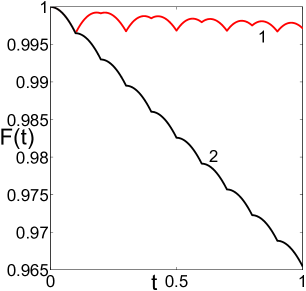
Figure 1: (Color online) Comparison of the fidelity evolution during $t=[0,\;1]$ of two methods for the superradiant state. We set $\tau=0.1$, $\lambda=2$ and $\Omega=1$. Line 2 is for dynamical decoupling of this work and Line 1 is for QZE of RefMan . The fidelity only oscillates in a small range around a horizontal line in the dynamical decoupling method.

III.2 Effect of finite duration of Double-$\pi$-Phase Operation

In practice, one cannot set the duration pulse time to be infinitely small. Here we consider the more realistic case that duration time of double-$\pi$-phase is finite and we study show the effect on the fidelity. We only consider the sequential pulses method and we suppose the pulse duration is $\tau\over N$ in each time interval $\tau$. We know that the decoherence coefficient of Superradiant state is Eqn. 22 when $t\in[m\tau,(m+1-{1\over N})\tau]$. So the effective Hamiltonian for the sequential double-$\pi$-phase operator is $H_{phase}={N\pi\over\tau}(\sigma^{+}_{1}\sigma^{-}_{1}+\sigma^{+}_{2}\sigma^{-}_{2})\sum_{m\geq 1}[\Theta(m\tau-{1\over N}\tau)-\Theta(m\tau)]$ and $\Theta(x)$ is the step function. Under the Hamiltonian $H_{all}=H_{s}+H_{e}+H_{i}+H_{phase}$, we can write down the state during the time of $[(m-{1\over N})\tau,m\tau]$:

$$\begin{split}|\psi(t)\rangle=&e^{-i{N\pi\over\tau}(t-(m-{1\over N})\tau)}(r(t)_{1}|1\rangle_{1}|0\rangle_{2}\\ &+r(t)_{2}|0\rangle_{1}|1\rangle_{2})\otimes|0\rangle_{e}\\ &+\sum_{k}|0\rangle_{1}|0\rangle_{2}\otimes c(t)_{k}|1_{k}\rangle_{e}\end{split}$$ (27)

In the same way as shown above, we also can get a integral equation describing the coefficient $\dot{r}_{1}=-\int_{0}^{t}d\tau f^{\prime}(t-\tau)[\alpha^{2}_{1}r_{1}(\tau)+\alpha_{1}\alpha_{2}r_{2}(\tau)]$ and the new correlation function of the duration time should be $f^{\prime}(t)=W^{2}e^{(-\lambda+i{N\pi\over\tau})t}$. Using the boundary condition of $t=(m-{1\over N})\tau$ and $t=m\tau$, we eliminate the coefficient in the operator’s duration time and get coupled relationships between $A_{m}$, $B_{m}$ and $A_{m+1}$, $B_{m+1}$(Eqn.22).

$$\begin{split}&e^{-{\lambda\over 2}(1-{1\over N})\tau}[A_{m}cosh({\Omega\over 2}(1-{1\over N})\tau)+B_{m}sinh({\Omega\over 2}(1-{1\over N})\tau)]\\ &=(1+\lambda{e^{\lambda\tau\over N}+1\over 4i\gamma-2\lambda})A_{m+1}-{e^{\lambda\tau\over N}+1\over 4i\gamma-2\lambda}\Omega B_{m+1}\\ &{\Omega\over\lambda}e^{-{\lambda\over 2}(1-{1\over N})\tau}[A_{m}sinh({\Omega\over 2}(1-{1\over N})\tau)+B_{m}cosh({\Omega\over 2}(1-{1\over N})\tau)\\ =&(1+e^{\lambda\tau\over N}+{\lambda\over 4i\gamma-2\lambda})A_{m+1}-({\Omega\over\lambda}e^{\lambda\tau\over N}+{\Omega\over 4i\gamma-2\lambda})B_{m+1}\end{split}$$ (28)

where $\gamma={N\pi\over 2\tau}$.

The time evolution of the system is given by $|\psi(t)\rangle=(\beta_{1}|\mu\rangle+\beta_{2}\xi(t)|\nu\rangle)\otimes|0\rangle_{e}+\sum_{k}|0\rangle_{1}|0\rangle_{2}\otimes c(t)_{k}|1_{k}\rangle_{e}$ and $\xi(t)$ is defined by Eqn. 22 with the new relation of $A_{m}$ and $B_{m}$ above. Also, the fidelity of the state under decoherence with the original state is

$$|\psi\rangle=(\beta_{1}|\mu\rangle+\beta_{2}|\nu\rangle)$$ (29)

$$F(t)=|\beta_{1}|^{2}+|\beta_{2}|^{2}\xi(t)$$ (30)

III.3 Numerical Calculation of Dynamical Decoupling and Free-evolution

Figure 2: (Color online) The initial state is the superradiant state. Line 2 is the fidelity under sequential double-$\pi$-phase method (Dynamical Decoupling). Line 3 is the fidelity under QZE. Line 1 is the fidelity of free-evolution under the interaction between system and environment. From the result, we can easily find the sequential-pulse method is much better than the QZE.

Figure 3: (Color online) The initial state is the superradiant state. Line 2 is the method with the instantaneous pulse. Line 4 is for $N=20$ and line 3 is for $N=10$. Line 1 is for the free-evolution.

In case 1, we set $\tau=0.1$, $\lambda=2$ and $\Omega=1$ and we compare the fidelity of the free-evolution, sequential double-$\pi$-phase operator and random one. The result is shown in Fig[2]. In case 2, we set $\tau=0.2$, $\lambda=2$, $\Omega=1$, $N_{1}=10$ and $N_{2}=20$ to compare how the duration time of pulses affect the fidelity. The result is shown in Fig[3].

IV Concluding remark

We present a strategy to protect the odd-parity states of two qubits under 0 temperature environment by frequently applying the $\pi-$pulses. Comparison between this method and the method based on frequent measurement is done, it seems that the frequent-$\pi-$pulses method is more effective in protecting the states. Our result clearly shows that the quantum Zeno effect and the dynamical decoupling can have rather different results when the operation frequency is finite, though the two methods give essentially the same results in the limit of infinite operation frequent as shown in Ref. Facchi1 ; Facchi2 ; Busch .
Acknowledgments XBW is supported by the National Natural Science Foundation of China under Grant No. 60725416, the National Fundamental Research Programs of China Grant No. 2007CB807900 and 2007CB807901, and China Hi-Tech Program Grant No. 2006AA01Z420. LCK acknowledges the financial support by the National Research Foundation & Ministry of Education.

References

- (1) P. telmachoni and V. Buzek, Phys. Rev. A 64, 062106 (2001)
- (2) A.G. Kofman and G. Kurizki, Phys. Rev. Lett. 93, 130406 (2004)
- (3) A. Einstein, B. Podolsky and N. Rosen, Phys. Rev. 47, 777 (1935)
- (4) C.H. Bennett, G. Brassard, C. Crepeau, R. Jozsa, A. Peres and W.K. Wootters, Phys. Rev. Lett. 70, 1895-1899(1993)
- (5) D.P. DiVincenzo, arXiv:cond-mat/9407022v1 (1994)
- (6) D.P. DiVincenzo and J. Smolin, arXiv:cond-mat/9409111v1 (1994)
- (7) Y. Makhlin, G. Schn and A. Shnirman, Rev. Mod. Phys. 73, 357-400 (2001)
- (8) Y.P. Huang and M.G. Moore, Phys. Rev. A 77, 062332 (2008)
- (9) L.M. Duan, M.D. Lukin, J.I. Cirac and P. Zoller, Nature 414, 413-418 (2001)
- (10) J.Z. Hu, Z.W. Yu and X.B Wang, Eur. Phys. J. D 51, 381 (2009)
- (11) L. Viola and S. Lloyd, Phys. Rev. A 58, 2733 (1998)
- (12) H.P. Breuer, B. Kappler and F. Petruccione, Phys. Rev. A 59, 1633 (1999)
- (13) D. Vitali and P. Tombesi, Phys. Rev. A 59, 4178 (1999)
- (14) G. Uhrig, Phys. Rev. Lett. 98, 100504 (2007); G. Uhrig, Phys. Rev. Lett. 102, 120502(2009)
- (15) W. Yang and R.B. Liu, Phys. Rev. Lett. 101, 180403 (2008)
- (16) F.F. Fanchini and R.d.J. Napolitano, Phys. Rev. A 76, 062306 (2007)
- (17) S. Maniscalco, F. Francica, R.L. Zaffino, N.L. Gullo and F. Plastina, Phys. Rev. Lett. 100, 090503 (2008)
- (18) J.R. West, B.H. Fong and D.A. Lidar, Phys. Rev. Lett. 104, 130501(2010)
- (19) J. Du et al, Nature 461, 1265 (2009)
- (20) M.J. Biercuk et al., Nature 458, 996 (2009)
- (21) H. Uys, M.J. Biercuk, and J.J. Bollinger, Phys. Rev. Lett. 103, 040501 (2009)
- (22) P. Facchi, D.A. Lidar and S. Pascazio, Phys. Rev. A 69, 032314(2004)
- (23) P. Facchi, S. Tasaki, S. Pascazio, H. Nakazato, A. Tokuse and D.A. Lidar, Phys. Rev. A 71, 022302(2005)
- (24) J. Busch and A. Beige, arXiv: 1002.3479
- (25) T. Yu and J.H. Eberly, Phys. Rev. Lett. 93, 140404 (2004); T. Yu and J.H. Eberly, Phys. Rev. Lett. 97, 140403 (2006)
- (26) M.P. Almeida et al., Science 316, 579 (2007)
- (27) G.M. Palma, K.-A. Suominen and A.K. Ekert, Proc. R. Soc. A 452,567 (1996)
- (28) P. Zanardi and M. Rasetti, Phys. Rev. Lett. 79, 3306 (1997)
- (29) M.O. Scully and M.S. Zubairy, Quantum Optics, Cambridge University Press
- (30) M. Tavis and F.W. Cummings, Phys. Rev. 170, 379 (1968)