Quantum Potentials with q-Gaussian Ground States

Abstract

We determine families of spherically symmetrical $D$-dimensional quantum potential functions $V(r)$ having ground state wavefunctions that exhibit, either in configuration or in momentum space, the form of an isotropic $q$-Gaussian. These wavefunctions admit a maximum entropy description in terms of $S_{q}$ power-law entropies. We show that the potentials with a ground state of the $q$-Gaussian form in momentum space admit the Coulomb potential $-1/r$ as a particular instance. Furthermore, all these potentials behave asymptotically as the Coulomb potential for large $r$ for all values of the parameter $q$ such that $0<q<1.$

I Introduction

Extended versions of the maximum entropy principle based upon power law $S_{q}$ entropies GT04 ; T09 have been found to provide useful tools for the description of several physical systems or processes GT04 ; T09 ; PP93a ; RPCP00 ; ASLMM05 ; PA97 . Indeed, various important equations in mathematical physics admit exact solutions of the maximum $S_{q}$ form such as, for example, the polytropic solutions to the Vlasov-Poisson equations PP93a , time dependent solutions to some evolution equations involving non linear, power-law diffusion terms RPCP00 ; ASLMM05 , or stationary phase-space distributions for Liouville equations describing anomalous thermostatting processes PA97 .

The application of information theoretical ideas to the study of the eigenstates of diverse quantum systems has attracted the attention of researchers in recent years MYD10 ; LAD09 ; GDPS09 ; DLOY06 ; RN08 ; DB09 ; NR09 ; PCPP95 . The standard maximum entropy principle, based on the optimization of Shannon’s entropic measure under appropriate constraints, plays a distinguished role within these lines of enquiry. This principle has been successfully applied to the characterization of the eigenstates of various quantum systems (see, for instance, NR09 ; PCPP95 ; PP93b and references therein). In particular, it is well known that the probability densities in both position and momentum space corresponding to the ground state of the isotropic $D$-dimensional quantum harmonic oscillator are Gaussians, which are probability densities maximizing Shannon’ entropy under the constraints imposed by normalization and the expectation value of the square $r^{2}$ of the radial coordinate.

It would be of considerable interest to extend to the $S_{q}$-based framework the maximum entropy approach to the description of the eigenstates of quantum systems. This formalism has already been applied to the study of various quantum phenomena (see, for example BCPP02 ; TBD98 ), but its application to characterize the probability densities associated with quantum eigenstates remains largely unexplored. The maximum entropy formalism based on the $S_{q}$ entropies leads to a generalization of the Gaussian probability density, which is given by the so-called $q$-Gaussians GT04 ; T09 . These $q$-Gaussian constitute some of the simplest and most important examples of maximum-$S_{q}$ distributions. The aim of the present work is to determine the form of those spherically symmetric quantum potentials $V(r)$ whose ground state wavefunctions (in position or in momentum space) are associated with $q$-Gaussian densities.

II q-Gaussian Ground States in Configuration Space

We are going to consider a spinless particle of mass $m$ in a $D$-dimensional configuration space. The eigenfunctions $\psi({\bf r})$ associated with a potential $V({\bf r})$ obey then the Schr dinger equation,

$$-\frac{\hbar^{2}}{2m}\nabla^{2}\psi+V\psi=E\psi,$$ (1)

where $\nabla^{2}$ is the $D$-dimensional Laplacian operator, $\hbar$ is Planck’s constant and $E$ is the energy eigenvalue. We assume in the rest of this paper that $m=\hbar=1$. Since we are going to consider spherically symmetric potentials, the Schr dinger equation for the concomitant ground states (which are spherically symmetric) simplifies to

$$-\frac{1}{2r^{D-1}}\frac{\partial}{\partial r}\left(r^{D-1}\frac{\partial\psi}{\partial r}\right)+V\psi=E\psi,$$ (2)

where

$$r=\left(\sum_{i=1}^{D}x_{i}^{2}\right)^{1/2}$$ (3)

is the radial coordinate.

Let us consider a $D-$dimensional spherical $q-$Gaussian wavefunction in the configuration space

$$\psi\left(\mathbf{r}\right)=C\left(1-\left(q-1\right)\beta r^{2}\right)^{\frac{1}{2\left(q-1\right)}}$$ (4)

where $q$ and $\beta$ are positive parameters and $C$ is an appropriate normalization constant. If $q<1$ the $q$-Gaussian wavefunction (4) remains finite for all ${\bf r}\in{\mathbb{R}}^{D}$. On the other hand, when $q>1$ the $q$-Gaussian vanishes at $r=1/\sqrt{(q-1)\beta}$ and is set to zero for $r>1/\sqrt{(q-1)\beta}$ (see below a discussion on the physical meaning of this cut-off). The space probability density $\rho({\bf r})=|\psi\left(\mathbf{r}\right)|^{2}$ associated with the wavefunction (4) maximizes Tsallis’ power-law entropic functional

$$S_{q}\,=\,\frac{1}{q-1}\,\left(1-\int\rho^{q}\,d{\bf r}\right)$$ (5)

under the constraints given by normalization and the expectation value of $r^{2}$ T09 (it can also be regarded as a probability density maximizing Rényi’s functional under the same constraints).

Replacing (4) into (1) and after some algebra, we find that the wavefunction is the ground state of the potential

$$V=\frac{\beta}{2}\left[\frac{-D+\beta r^{2}\left(D\left(q-1\right)+3-2q\right)}{\left(1-\left(q-1\right)\beta r^{2}\right)^{2}}\right]$$ (6)

with eigenenergy equal to $0.$

In the case $q\leq 1$ the potential function (6) is finite for all ${\bf r}\in{\mathbb{R}}^{D}$. On the other hand, when $q>1$ the potential function is singular when $r$ adopts the particular value

$$r_{w}\,=\,\sqrt{\frac{1}{(q-1)\beta}}.$$ (7)

Physically, this means that when $q>1$ the potential function (6) has an “infinite wall" at $r=r_{w}$ and the quantum particle is confined within the region $r\leq r_{w}$. In this case, the $q$-Gaussian wavefunction (4) vanishes at $r=r_{w}$ and must be set equal to zero when $r\geq r_{w}$. This constitutes an example of the so-called Tsallis’ cut-of condition T09 ; PP93a .

In the limit $q\rightarrow 1$ the $q$-Gaussian wavefunction (4) becomes a standard Gaussian, and the potential function (6) reduces to the $D$-dimensioanl isotropic harmonic oscillator potential (notice that the origin of the energy scale is shifted)

$$V(r)\,=\,-\frac{D\beta}{2}+\frac{1}{2}\beta^{2}r^{2}.$$ (8)

The one dimensional instance of the potential (6) has been studied in RPGCP00 . This potential exhibits the interesting feature of approximate shape invariance (see RPGCP00 for details). This approximate symmetry becomes exact in the limit $q\rightarrow 1$.

III q-Gaussian ground states in momentum space

We now look for solutions solution of the Schr dinger equation having the form of a $q-$Gaussian in momentum space

$$\tilde{\psi}\left(\mathbf{p}\right)=C\left(1-\left(q-1\right)\beta p^{2}\right)^{\frac{1}{2\left(q-1\right)}}$$ (9)

where

$$p^{2}=\sum_{i=1}^{D}p_{i}^{2}.$$ (10)

As in the previous case of $q$-Gaussians in configuration space, $q$ and $\beta$ are positive parameters and $C$ is a normalization constant. We are going to consider $q$-Gaussians in momentum space with $q<1$. Our aim is to determine potential functions $V(r)$ having a ground state that, in momentum space, has the form (9). In order to do this, it will prove convenient not to work directly with the Schr dinger equation in momentum space but, instead, to determine first the Fourier transform $\psi\left(\mathbf{r}\right)$ of $\tilde{\psi}\left(\mathbf{p}\right)$ and then to consider Schr dinger’s equation in configuration space.

The Fourier transform of the $q-$Gaussian wave function (9) is

$$\psi_{\nu}\left(\mathbf{r}\right)=\frac{2^{1-\nu}}{\Gamma\left(\nu\right)}r^{\nu}K_{\nu}\left(r\right)$$ (11)

where $K_{\nu}$ is the Bessel function of the second kind and $r=|\mathbf{r}|.$ The parameter parameter $\nu$ is given by

$$\nu=-\frac{D}{2}-\frac{1}{2\left(q-1\right)}.$$ (12)

Theorem.

The function $\psi_{\nu}\left(r\right)$ is solution of the Schr dinger equation associated with a potential

$$V_{\nu}\left(r\right)=-\frac{1}{2}\,\left(1+\frac{D}{2\left(\nu-1\right)}\right)\frac{\psi_{\nu-1}\left(r\right)}{\psi_{\nu}\left(r\right)}.$$ (13)

As a special case, when the parameter $\nu=d+\frac{1}{2}$ is half integer, this potential is of the form

$$V_{d+\frac{1}{2}}\left(r\right)=-\frac{1}{2}\,\left(1+\frac{D}{2d-1}\right)\frac{p_{d-1}\left(r\right)}{p_{d}\left(r\right)}$$ (14)

where $p_{d}\left(r\right)$ is the Bessel polynomial of degree $d.$

Proof.

The derivation rule for the function $\psi\left(r\right)$ is

$$\frac{1}{r}\frac{\partial}{\partial r}\psi_{\nu}\left(r\right)=-\frac{1}{2\left(\nu-1\right)}\psi_{\nu-1}\left(r\right)$$ (15)

so that the Laplace operator reads

$$\frac{1}{r^{D-1}}\frac{\partial}{\partial r}\left(r^{D-1}\frac{\partial\psi_{\nu}}{\partial r}\right)=\frac{1}{r^{D-1}}\left(\left(D-1\right)r^{D-2}\frac{\partial\psi_{\nu}}{\partial r}+r^{D-1}\frac{\partial^{2}\psi_{\nu}}{\partial r^{2}}\right)$$ (16)

The first term is

$$-\frac{\left(D-1\right)}{2\left(\nu-1\right)}\psi_{\nu-1}\left(r\right)$$ (17)

and the second term

$$\frac{\partial^{2}\psi_{\nu}}{\partial r^{2}}=-\frac{1}{2\left(\nu-1\right)}\frac{\partial}{\partial r}\left(r\psi_{\nu-1}\left(r\right)\right)=-\frac{1}{2\left(\nu-1\right)}\psi_{\nu-1}\left(r\right)+\frac{1}{4\left(\nu-1\right)\left(\nu-2\right)}r^{2}\psi_{\nu-2}\left(r\right)$$ (18)

so that the Laplace operator applied to $\psi_{\nu}$ is

$$\frac{1}{r^{D-1}}\frac{\partial}{\partial r}\left(r^{D-1}\frac{\partial\psi_{\nu}}{\partial r}\right)=\left(-\frac{D}{2\left(\nu-1\right)}\psi_{\nu-1}\left(r\right)+\frac{1}{4\left(\nu-1\right)\left(\nu-2\right)}r^{2}\psi_{\nu-2}\left(r\right)\right)$$ (19)

Moreover, the function Bessel function $K_{\nu}$ obeys the difference equation

$$rK_{\nu}\left(r\right)=rK_{\nu-2}\left(r\right)+2\left(\nu-1\right)K_{\nu-1}\left(r\right)$$ (20)

so that

$$r^{\nu}K_{\nu}\left(r\right)=r^{2}r^{\nu-2}K_{\nu-2}\left(r\right)+2\left(\nu-1\right)r^{\nu-1}K_{\nu-1}\left(r\right)$$ (21)

and

$$\psi_{\nu}\left(r\right)=r^{2}\frac{1}{4\left(\nu-1\right)\left(\nu-2\right)}\psi_{\nu-2}\left(r\right)+\psi_{\nu-1}\left(r\right).$$ (22)

We deduce

$$\Delta\psi_{\nu}\left(r\right)=\frac{1}{r^{D-1}}\frac{\partial}{\partial r}\left(r^{D-1}\frac{\partial\psi_{\nu}}{\partial r}\right)=\left(-\frac{D}{2\left(\nu-1\right)}-1\right)\psi_{\nu-1}\left(r\right)+\psi_{\nu}\left(r\right).$$ (23)

Consequently,

$$-\frac{1}{2}\Delta\psi_{\nu}\left(r\right)+\left[-\frac{1}{2}\left(1+\frac{D}{2\left(\nu-1\right)}\right)\frac{\psi_{\nu-1}\left(r\right)}{\psi_{\nu}\left(r\right)}\right]\,\psi_{\nu}\left(r\right)\,=\,-\frac{1}{2}\,\psi_{\nu}\left(r\right),$$ (24)

which means that $\psi_{\nu}\left(r\right)$ is an eigenfunction of the potential $V_{\nu}(r)$ given by equation (13), with eigenvalue equal to $-\frac{1}{2}$.

∎

IV Special cases and asymptotics

IV.1 Asymptotics

The asymptotics for large $r$ of the potential (13) can be computed using (Abramowitz, , 9.7.2)

$$K_{\nu}\left(r\right)\sim\sqrt{\frac{\pi}{2r}}e^{-r}\left(1+\frac{4\nu^{2}-1}{8r}+\dots\right)$$ (25)

so that the asymptotics for the potential (13) reads

$$V_{\nu}\left(r\right)\sim-\frac{\left(2\left(\nu-1\right)+D\right)}{r}\left(1+\frac{1}{2r}\left(1-2\nu\right)+\dots\right).$$ (26)

We see then that, for large values of $r$, the asymptotic behavior of the potential $V_{\nu}\left(r\right)$ is dominated by a Coulomb-like term.

IV.2 Special cases

1. Coulomb potential: taking $\nu=\frac{1}{2}$ and remarking that $\psi_{\frac{1}{2}}\left(r\right)=\exp\left(-r\right)$ and $\psi_{-\frac{1}{2}}\left(r\right)=-\frac{1}{r}\psi_{\frac{1}{2}}\left(r\right),$ we deduce that

   $$-\frac{1}{2}\Delta\psi_{\frac{1}{2}}\left(r\right)-\frac{D-1}{2r}\psi_{\frac{1}{2}}\left(r\right)=-\frac{1}{2}\psi_{\frac{1}{2}}\left(r\right)$$ (27)

   which is the Schr dinger equation associated with a Coulomb potential. The associated probability density in configurational space can be obtained as the squared modulus of the inverse Fourier transform of the ground state wavefunction in momentum space,

   $$\tilde{\psi}_{\frac{1}{2}}\left(\mathbf{p}\right)\propto\left(1+|\mathbf{p}|^{2}\right)^{-\frac{D+1}{2}}.$$ (28)

   The momentum space representation of the eigenfunctions corresponding to the $D$-dimensional Coulomb potential have been studied in detail by Aquilanti, Cavalli and Coletti in aquilanti .

   The $q$-value characterizing the ground state of the $-\frac{1}{r}$ potential is different from one. Indeed, it depends on the value of the space dimension $D$,

   $$q\,=\,\frac{D}{D+1}.$$ (29)

2. In Table I we give a few potentials resulting from different half integer values of $\nu$. These potentials are depicted in Fig.1. If $\nu=\frac{1}{2}+d$, with $d$ integer, then the entropic parameter $q$ characterizing the $q$-Gaussian is given by

   $$q\,=\,\frac{D+2d}{D+2d+1}.$$ (30)

   It is interesting that, for a given fixed value of $d$, we have that $q\rightarrow 1$ when $D\rightarrow\infty$. That is, when the space dimension tends to infinity the $q$-Gaussian describing the ground state in momentum space approaches a standard Gaussian.

   $\nu$	$\frac{3}{2}$	$\frac{5}{2}$	$\frac{7}{2}$
   $V_{\nu}\left(r\right)$	$-\frac{1}{2}\left[\frac{1+D}{1+r}\right]$	$-\frac{1}{2}\left[\frac{\left(3+D\right)\left(r+1\right)}{r^{2}+3r+3}\right]$	$-\frac{1}{2}\left[\frac{\left(5+D\right)\left(r^{2}+3r+3\right)}{r^{3}+6r^{2}+15r+15}\right]$

   Table 1: Values of the potential for different half-integer values of the parameter $\nu$

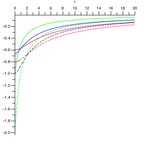
Figure 1: The potential functions $V_{\nu}$ appearing in Table I, corresponding to $\nu$ equal to $\frac{3}{2}$, $\frac{5}{3}$ and $\frac{7}{2}$ (top to bottom), for $D=1$ (solid line) and $D=3$ (dashed line).

V Conclusions

We have determined the $D$-dimensional spherically symmetric potential functions having ground states of the $q$-gaussian form, either in configuration or in momentum space. In the case of $q$-gaussian ground states in configuration space we obtained a bi-parametric family of potentials admitting the $D$-dimensional isotropic harmonic oscillator as the particular case corresponding to the limit $q\rightarrow 1$. On the other hand, when considering ground states having the shape of a q-Gaussian in momentum space we obtained a family of potentials closely related to the $D$-dimensional Coulomb (or Hydrogen) potential $-\frac{1}{r}$. In point of fact, this family admits the standard ($D$-dimensional) Coulomb potential itself as a particular instance. Moreover, for large values of $r$, all the above mentioned potentials behave asymptotically as $-\frac{1}{r}$ for all $0<q<1$.

Within classical mechanics, it is already well known that there is a close relationship between the potential function $-\frac{1}{r}$ (describing Newtonian gravitation) and maximum $S_{q}$ distributions. The celebrated polytropic solutions of the Vlasov-Poisson equations, widely used in the study of self-gravitating astrophysical systems, have indeed the $S_{q}$-maxent form, and the associated velocity distributions are $q$-Gaussians. It is an intriguing fact that, as we have shown in the present work, there also exits a close connection between $q$-Gaussians and the $-\frac{1}{r}$ potential in quantum mechanics.

Acknowledgments. This work was partially supported by by the Project FQM-2445 of the Junta de Andalucía and by the Grant FIS2008-2380 of the Ministerio de Innovación y Ciencia, Spain.

References

- (1) M. Gell-Mann and C. Tsallis, Eds. Nonextensive Entropy: Interdisciplinary applications, Oxford University Press, Oxford, 2004.
- (2) C. Tsallis, Introduction to Nonextensive Statistical Mechanics: Approaching a Complex World, Springer, New York, 2009.
- (3) A.R. Plastino and A. Plastino, Phys. Lett. A 174 (1993) 384.
- (4) A. Rigo, A.R. Plastino, M. Casas, and A. Plastino, Phys. Lett. A 276 (2000) 97.
- (5) P.C. Assis, L.R. da Silva, E.K. Lenzi, L.C. Malacarne and R.S. Mendes, J. Math. Phys. 46 (2005) 123303.
- (6) A.R. Plastino and C. Anteneodo, Annals of Physics 255 (1997) 250.
- (7) D. Manzano, R. Y ez and J.S. Dehesa, New Journal of Physics 12 (2010) 023014.
- (8) S. L pez-Rosa, J.C. Angulo and J.S. Dehesa, Eur. Phys. Journ. D 51 (2009) 321.
- (9) R. Gonz lez-F rez, J.S. Dehesa, S.H. Patil and K.D. Sen, Physica A 388 (2009) 4919.
- (10) J.S. Dehesa, S. L pez-Rosa, B. Olmos and R.J. Y ez, J. Math. Phys. 47 (2006) 052104.
- (11) E. Romera and . Nagy Phys. Lett. A 372 (2008) 4918.
- (12) C. Das and K. Bhattacharyya, Phys. Rev. A 79 (2009) 012107.
- (13) A. Nagy and E. Romera, Phys. Lett. A 373 (2009) 844.
- (14) A.R. Plastino, M. Casas, A. Plastino and A. Puente, Phys. Rev. 52 (1995) 2601.
- (15) A.R. Plastino and A. Plastino, Phys. Lett. A 181 (1993) 446.
- (16) J. Batle, M. Casas, A.R. Plastino, and A. Plastino, Phys. Lett. A 296 (2002) 251.
- (17) U. Tirnakli, F. B y kkili and D. Demirhan, Phys. Lett. A 245 (1998) 62.
- (18) A. Rigo, A. R. Plastino, F. Garcias, M. Casas and A. Plastino, J. Phys. A: Math. Gen. 33 (2000) 6457.
- (19) M. Abramowitz and I.A. Stegun, Handbook of Mathematical Functions with Formulas, Graphs, and Mathematical Tables, Dover Publications, 1972.
- (20) V. Aquilanti, S. Cavalli, C. Coletti, Chemical Physics 2 ( 1997) 1.