Optimal designs for random effect models with correlated errors with applications in population pharmacokinetics

Abstract

We consider the problem of constructing optimal designs for population pharmacokinetics which use random effect models. It is common practice in the design of experiments in such studies to assume uncorrelated errors for each subject. In the present paper a new approach is introduced to determine efficient designs for nonlinear least squares estimation which addresses the problem of correlation between observations corresponding to the same subject. We use asymptotic arguments to derive optimal design densities, and the designs for finite sample sizes are constructed from the quantiles of the corresponding optimal distribution function. It is demonstrated that compared to the optimal exact designs, whose determination is a hard numerical problem, these designs are very efficient. Alternatively, the designs derived from asymptotic theory could be used as starting designs for the numerical computation of exact optimal designs. Several examples of linear and nonlinear models are presented in order to illustrate the methodology. In particular, it is demonstrated that naively chosen equally spaced designs may lead to less accurate estimation.

T1Supported by Deutsche Forschungsgemeinschaft (SFB 823, “Statistik nichtlinearer dynamischer Prozesse.” Teilprojekt C2).

, and t2Supported in part by NIH Grant IR01GM072876:01A1 and the BMBF project SKAVOE.

1 Introduction

The work presented in this paper is motivated by some problems encountered in the design of experiments in a clinical trial to establish the pharmacokinetics of Uzara®, a digitoxin related herbal diarrhea medication [based on Thürmann, Neff and Fleisch (2004)]. These kinds of trials pose methodological design challenges because they require the estimation of global population parameters in the presence of correlated measurement errors. The trial in question included a number of patients each given an oral application of Uzara® as well as, after a washout period, an intravenous application of digoxin (Lanicor®), where in both cases the resulting serum concentration of digitoxin was measured repeatedly during the next $36$ hours.

The relation between the time and the concentration in the analysis of the Uzara® trial can be described using the theory of one-compartment models with oral and, respectively, intravenous applications [Atkinson et al. (1993), Shargel (1993)]. In the intravenous case, the medication reaches the maximum concentration in the blood almost immediately, and, after that, it is gradually eliminated from the body over time. Thus, the digitoxin concentration is modeled using the exponential elimination model

$$\eta(t,b)=b_{1}e^{-b_{2}t}.$$ (1)

In the case of the oral application, there is a gradual build up of the concentration in the blood as the medication is absorbed through the digestive tract, while there is a simultaneous elimination process of the medication in the blood. Therefore, the concentration function is the solution of the differential equation of these two parallel processes. The resulting function

$$\eta(t,b)=b_{3}(e^{-b_{1}t}-e^{-b_{2}t})$$ (2)

is known as the ($3$ parameter) Bateman function [Garrett (1994)]. In both models, the function $\eta(t,b)$ denotes the concentration function, $t$ is the time (in hours), $b=(b_{1},b_{2})$ and, respectively, $b=(b_{1},b_{2},b_{3})$ are the vectors of parameters. The parameters are assumed to vary between patients and the aim of the experiment is to estimate their global means (and sometimes variances) over all patients.

Measurements within the same patient are usually correlated, and we assume this correlation to be proportional to the time lag between measurements, which is plausible as the random errors are usually caused by temporary changes in the patients physical condition. Measurements for different patients are assumed to be independent. In the trial at question Thuermann considered $n=15$ (oral), respectively, $n=14$ (intravenous) measurements each on $K=18$ patients. After a preliminary discussion with experts the measurements were taken at nonoptimized time points. An approximation of the covariance of a single patient can then be expressed as

$$\Sigma_{\mathit{pop}}=\frac{\partial\eta(\mathbf{t},b)}{\partial b}^{T}V_{p}\frac{\partial\eta(\mathbf{t},b)}{\partial b}+V_{\varepsilon},$$ (3)

where $\eta(\mathbf{t},b)=(\eta(t_{1},b),\ldots,\eta(t_{n},b))^{T}$ denotes the vector of expected responses at $t_{1},\ldots,t_{n}$ and $V_{\varepsilon}$ is the covariance matrix corresponding to this data. This expression includes two sources of variation, the usual variation $V_{\varepsilon}$ caused by random errors as well as the additional variation $V_{p}$ due to the random effect.

Situations of this kind are rather common in the evaluation of the pharmacokinetics and the pharmacodynamics of drugs [see Buelga et al. (2005), Colombo et al. (2006), among others]. The corresponding processes are usually modeled by linear or nonlinear random effects models, which try to estimate the population parameters, that is, the mean and the inter-individual variability of the parameters. Under the additional assumption of a normal distribution, the population characteristics are usually estimated by maximum likelihood methods. In many cases, the likelihood cannot be evaluated explicitly and approximations are used to calculate the estimate. Efficient algorithms for estimation are available for this purpose [see Aarons (1999)]. Loosely speaking, under a Gaussian assumption this approach corresponds to weighted nonlinear least squares estimation. It was pointed out by several authors that the application of an appropriate design in these studies can substantially increase the accuracy of estimation of the population parameters. Usually, the construction of a good design is based on the Fisher information matrix which cannot be derived explicitly in pharmacokinetic models with random effects. For this reason, many authors propose an approximation of the likelihood [see, e.g., Mentré, Mallet and Baccar (1997), Retout, Mentré and Bruno (2002), Retout and Mentré (2003), Schmelter (2007a, 2007b), among others], which is used to derive an approximation for the Fisher information matrix. This matrix is considered in various optimality criteria, which have been proposed for the construction of optimal designs for random effect regression models.

In the present paper the investigation is motivated by the following issues. First, the estimation of the population mean and the construction of corresponding optimal designs for population pharmacokinetics strongly depends on the Gaussian assumption, which is usually made for computational convenience. Moreover, the maximum likelihood estimates may be inconsistent if the basic distributional assumption is violated. As a consequence, the derived optimal designs might be inefficient. Second, most authors derive the approximation for the Fisher information matrix under the additional assumption that the random errors corresponding to the measurements of each individual are uncorrelated [see, e.g., Retout, Duffull and Mentre (2001), Retout, Mentré and Bruno (2002) and Retout and Mentré (2003), among many others]. However, this assumption is not realistic in many applications of population pharmacokinetics. Thus, a general concept for constructing optimal designs in the presence of correlated observations is still missing. Third, even if the Gaussian assumption and the assumption of uncorrelated errors for each subject can be justified, the numerical construction of the estimate and the corresponding optimal design is extremely hard.

In the present paper we address these issues. To derive a good design, we consider nonlinear least squares estimation in random effect regression models. Note that this estimation does not require a specification of the underlying distributions. For this estimation, we introduce a methodology which can be used to derive efficient or optimal designs in very general situations. More precisely, we embed the discrete optimal design problem in a continuous optimal design problem, where a nonlinear functional of the design density has to be minimized or maximized. This approach takes into account the correlation dependence and yields an asymptotic optimal design density, which has to be determined numerically in all cases of practical interest. For finding the optimal density, we propose an algorithm based on polynomial approximation. For a fixed sample size and for each individual, an exact design can be obtained from the quantiles of the corresponding optimal distribution function. It is demonstrated by examples that these designs are very efficient. Moreover, the designs, derived from the asymptotic optimal design density, are very good starting designs for any procedure of local optimization for finding the exact optimal designs. To our knowledge, the proposed method is the first systematic approach to determine optimal designs for linear and nonlinear mixed effect models with correlated errors.

The remaining part of this paper is organized as follows. In Section 2 we consider the case of a linear random effect model and explain the basic design concepts. In Section 3 we introduce the approach for deriving the asymptotic optimal designs for linear regression models with correlated observations by employing results of Bickel and Herzberg (1979). In Section 4 we present results for nonlinear regression models with correlated random errors and derive $D$-optimal designs and optimal designs for estimating the area under the curve in the compartmental model. Finally, the Uzara® and Lanicor® trials are re-analyzed and optimal designs for the model (2) are determined. In particular, we show that the design proposed by the experts is rather efficient, while a naively chosen equidistant design can yield substantially less accurate estimates.

2 Statement of the problem

Consider the common random effect linear regression model

$$Y_{ij}=b_{i}^{T}g(t_{ij})+\varepsilon_{ij},\qquad i=1,\ldots,K;j=1,\ldots,n_{i},$$ (4)

where $Y_{ij}$ denotes the $j$th observation of the $i$th subject at the experimental condition $t_{ij}$, $\varepsilon_{11},\ldots,\varepsilon_{K,n_{K}}$ are centered random variables with variances depending on $t$, $\operatorname{Var}(\varepsilon_{ij})=\sigma^{2}h^{2}(t_{ij})$ for some positive function $h(t)$, $g(t)=(g_{1}(t),\ldots,g_{p}(t))^{T}$ is a given vector of linearly independent regression functions, and $b_{i}$ is a $p$-dimensional random vector representing the individual parameters of the $i$th subject, $i=1,\ldots,K$. The explanatory variables $t_{ij}$ can be chosen by the experimenter from a compact interval $T$. We assume that errors $\varepsilon_{i}=(\varepsilon_{i1},\ldots,\varepsilon_{in_{i}})$ for different subjects are independent, but the errors for the same subject are correlated, that is,

$$\operatorname{Cov}(\varepsilon_{ij},\varepsilon_{is})=\sigma^{2}h(t_{ij})h(t_{is})\bigl{(}\gamma r(t_{ij}-t_{is})+(1-\gamma)\delta_{{j},{s}}\bigr{)},$$ (5)

where $\gamma\in[0,1]$ is a constant, $r(t)$ is a given correlation function such that $r(0)=1$, and $\delta_{{j},{s}}$ denotes Kronecker’s symbol. Let $V_{\varepsilon}$ be the corresponding covariance matrix. Assume that the individual parameters $b_{i}$ are drawn from a population distribution with mean $\beta$ and covariance matrix $V_{p}$, and they are independent of the random variables $\varepsilon_{i}$. This means that the covariance between two observations at the time $t_{ij}$ and the time $t_{is}$ ($j\neq s$) is

$$\operatorname{Cov}(Y_{ij},Y_{is})=g^{T}(t_{ij})V_{p}g(t_{is})+\sigma^{2}h(t_{ij})h(t_{is})\gamma r(t_{ij}-t_{is}),$$

while the variance of $Y_{ij}$ is given by $g^{T}(t_{ij})V_{p}g(t_{ij})+\sigma^{2}h^{2}(t_{ij})$. It was shown by Schmelter (2007b) that an optimal design necessarily advises the experimenter to perform observations of all subjects at the same experimental settings, that is, $t_{ij}=t_{j}$ ($i=1,\ldots,K$, $j=1,\ldots,n$). Consequently, we define an exact design $\xi=\{t_{1},\ldots,t_{n}\}$ as an $n$-dimensional vector which describes the experimental conditions for each subject. Without loss of generality, we assume that the design points are ordered, $t_{1}<\cdots<t_{n}$.

Suppose that $n$ observations are taken according to the design $\xi$. Then the model (4) for the $i$th subject can be written as

$${Y}_{i}=X_{g}b_{i}+{\varepsilon}_{i};\qquad i=1,\ldots,K,$$ (6)

where ${Y}_{i}=(Y_{i1},\ldots,Y_{in})^{T}$, the matrix $X_{g}$ is given by $X_{g}=(g(t_{1}),\ldots,g(t_{n}))^{T}$, and ${\varepsilon}_{i}$ is now a centered random variable with variance $\sigma^{2}h^{2}(t_{i})$. This model is a special case of the random-effect models discussed in Harville (1976), which are called generalized MANOVA. According to Fedorov and Hackl (1997), the (ordinary) least square estimate of $\beta$ minimizes

$$\sum_{i=1}^{K}\sum_{j=1}^{n}h^{-2}(t_{j})\bigl{(}Y_{ij}-f(t_{j})\beta\bigr{)}^{2}.$$

Define $f(t)=g(t)/h(t)$ and $X=(f(t_{1}),\ldots,f(t_{n}))^{T}$. Then the covariance matrix of the ordinary least squares estimate $\hat{\beta}_{\mathrm{OLS}}$ is given by

$$\mathbf{D}(\hat{\beta}_{\mathrm{OLS}}) = \frac{1}{K}(X^{T}X)^{-1}X^{T}(V_{\varepsilon}+XV_{p}X^{T})X(X^{T}X)^{-1}$$

$$= \frac{1}{K}\bigl{(}(X^{T}X)^{-1}X^{T}V_{\varepsilon}X(X^{T}X)^{-1}+V_{p}\bigr{)}.$$

Alternatively, if the covariance matrix $V_{\varepsilon}$ of the errors and the covariance matrix of the random effects $V_{p}$ were known (or can be well estimated), the (weighted) least squares statistic

$$\quad\hat{\beta}_{\mathrm{WLS}}=\frac{1}{K}\sum_{i=1}^{K}\bigl{(}X^{T}(V_{\varepsilon}+XV_{p}X^{T})^{-1}X\bigr{)}^{-1}X^{T}(V_{\varepsilon}+XV_{p}X^{T})^{-1}Y_{i},$$ (8)

can be used to estimate the parameter $\beta$. The covariance matrix of the estimate $\hat{\beta}_{\mathrm{WLS}}$ is given by

$$\mathbf{D}(\hat{\beta}_{\mathrm{WLS}})=\frac{1}{K}\bigl{(}X^{T}(V_{\varepsilon}+XV_{p}X^{T})^{-1}X\bigr{)}^{-1}.$$ (9)

Since the expression (2) is simpler than (9) (which requires two different inversions), the design methodology developed in this paper is based on the covariance matrix of the ordinary least squares estimate. Additionally, we will demonstrate that the optimal designs obtained by minimizing functionals of the covariance matrix of the ordinary least squares estimate are also very efficient for weighted least squares estimation.

We call a design optimal design if it minimizes an appropriate functional of the covariance matrix of the least squares estimate. Since we consider optimality criteria that are linear with respect to scalar multiplication of the covariance matrix, we put $K=1$ without loss of generality.

3 Asymptotic optimal designs

Although the theory of optimal design has been discussed intensively for uncorrelated observations [see, e.g., Fedorov (1972), Pázman (1986) and Atkinson and Donev (1992)], less results can be found for dependent observations. For linear and nonlinear random effect models, optimal designs under the assumption of uncorrelated errors have been investigated in Schmelter (2007a, 2007b), Mentré, Mallet and Baccar (1997) and Retout and Mentré (2003), among others. For fixed effect regression models with the presence of correlated errors, it was suggested to derive optimal designs by asymptotic considerations. Sacks and Ylvisaker (1966, 1968) have considered a fixed design space, where the number of design points in this set tends to infinity. As a result, the asymptotic optimal designs depend only on the behavior of the correlation function in a neighborhood of the point $0$. In the present paper we use the approach of Bickel and Herzberg (1979) and Bickel, Herzberg and Schilling (1981), who have considered a design interval expanding proportionally to the number of observation points. This case is equivalent to the consideration of a fixed interval with the correlation function depending on the sample size. To be precise, we assume that the design space is given by an interval $T$ and the design points of a sequence of designs $\xi_{n}=\{t_{1n},\ldots,t_{nn}\}$ are generated by a function $a(\cdot)$ in the form

$$t_{jn}=a\bigl{(}(j-1)/(n-1)\bigr{)},\qquad j=1,\ldots,n;$$ (10)

and $a\dvtx[0,1]\to T$ denotes the inverse of a distribution function. Note that the function $a(\cdot)$ is obtained from the density of the weak limit of the sequence $\xi_{n}$ as $n\to\infty$. For example, if $T=[-1,1]$, the function $a(u)=(2u-1)$ corresponds to the equally-spaced designs with distribution function $a^{-1}(x)=\frac{x+1}{2}$ and density $(a^{-1})^{\prime}(x)=\frac{1}{2}I_{[-1,1]}(x)$. Furthermore, we assume that the correlation function $r(t)$ of the errors $\varepsilon_{i}$ in (5) depends on $n$ in the form

$$r_{n}(t)=\rho(nt),$$ (11)

such that $\rho(t)=o(t)$ as $t\to\infty$. For the numerical construction of asymptotic optimal designs, we derive an asymptotic representation for the covariance matrix of the least squares estimate in the following lemma. For this purpose, we impose the following regularity assumptions:

1. [(C3)]

2. The functions $f_{1}(t),\ldots,f_{p}(t)$ are linearly independent, bounded on the interval $T$ and satisfy the first order Lipschitz condition:

   $$|f_{i}(t)-f_{i}(s)| \leq M|t-s|\quad\mbox{and}$$

   $$|f_{i}(t)| \leq M\qquad\mbox{for all }t,s\in T,i=1,\ldots,p.$$

3. The function $a(\cdot)$ is twice differentiable and there exists a positive constant $M<\infty$ such that for all $u\in(0,1)$,

   $$\frac{1}{M}\leq a^{\prime}(u)\leq M,\qquad|a^{\prime\prime}(u)|\leq M.$$ (12)

4. The correlation function $\rho$ is differentiable with bounded derivative and satisfies $\rho^{\prime}(t)\leq 0$ for sufficiently large $t$.

Assumption (C1) refers to the continuity of the response as a function of $t$ and it is satisfied for most of the commonly used regression models. Moreover, most of the commonly used correlation structures satisfy assumption (C3) on a compact interval. Finally, assumption (C2) refers to the characteristics of a design, requiring, loosely speaking, that observations should not be clustered. This is quite reasonable due to ethical aspects. The following result is obtained by similar arguments as given in Bickel and Herzberg (1979) and, hence, its proof is omitted.

Assuming that conditions (C1), (C2) and (C3) are satisfied, then the covariance matrix of the least squares estimate have the form

$$\quad\mathbf{D}(\hat{\beta}_{\mathrm{OLS}})=\frac{\sigma^{2}}{n}\bigl{(}W^{-1}(a)+2\gamma W^{-1}(a)R(a)W^{-1}(a)\bigr{)}+V_{p}+o\biggl{(}\frac{1}{n}\biggr{)},$$ (13)

where the matrices $W(a)$ and $R(a)$ are defined by

$$W(a) = \biggl{(}\int_{0}^{1}f_{i}(a(u))f_{j}(a(u))\,du\biggr{)}_{i,j=1}^{p},$$

$$R(a) = \biggl{(}\int_{0}^{1}f_{i}(a(u))f_{j}(a(u))Q(a^{\prime}(u))\,du\biggr{)}_{i,j=1}^{p}$$

and the function $Q(\cdot)$ is given by $Q(t)=\sum_{j=1}^{\infty}\rho(jt).$

Note that only the first term in (2) [and (13)] depends on a (asymptotic) design, and we propose to use this term for the construction of optimal designs. If the function $a(\cdot)$ is the inverse of a continuous distribution with density, say, $\varphi$, then $a^{\prime}(t)=1/\varphi(t)$ and, for large $n$, the first term of the covariance matrix can be approximated by the matrix $V(\varphi)/n$, where the $p\times p$ matrix $V$ is given by

$$V(\varphi) := \sigma^{2}\bigl{(}W^{-1}(\varphi)+2\gamma W^{-1}(\varphi)R(\varphi)W^{-1}(\varphi)\bigr{)}.$$ (14)

In (14) the matrices $W(\varphi)$ and $R(\varphi)$ have the form

$$W(\varphi) = \biggl{(}\int_{T}f_{i}(t)f_{j}(t)\varphi(t)\,dt\biggr{)}_{i,j=1}^{p},$$

$$R(\varphi) = \biggl{(}\int_{T}f_{i}(t)f_{j}(t)Q\bigl{(}1/\varphi(t)\bigr{)}\varphi(t)\,dt\biggr{)}_{i,j=1}^{p}.$$

A density will be called an asymptotic optimal density $\varphi^{*}$, if it minimizes an appropriate functional of the matrix $V(\varphi)$. Numerous criteria have been proposed in [Silvey (1980), Atkinson and Donev (1992), Pukelsheim (1993)] and, exemplarily, we consider the $D$- and $c$-optimality criteria which minimize $-\det V(\varphi)$ and $c^{T}V(\varphi)c$ for a given vector $c\in\mathbb{R}^{p}$, respectively. The application of the proposed methodology to other optimality criteria is straightforward. The general procedure for constructing an efficient design minimizing a given functional of the covariance matrix of the least squares estimate is as follows:

1. [(3)]

2. Specify the correlation function $\rho(\cdot)$ in (11) and compute $Q(\cdot)$.

3. Compute the asymptotic optimal design density $\varphi^{*}$ that minimizes an appropriate functional of the matrix $V(\varphi)$ in (14).

4. Derive the exact design for a fixed sample size $n$ by calculation of the quantiles of the distribution function $\Phi^{*}$ that corresponds to $\varphi^{*}$, namely,

   $$t_{i,n}=(\Phi^{*})^{-1}\biggl{(}{i-1\over n-1}\biggr{)};\qquad i=1,\ldots,n.$$ (15)

The optimal density $\varphi^{*}$ in step (2) can be determined as follows. We consider the parametric representation of a density by a polynomial in the form

$$\varphi(t)=\frac{(p_{0}+p_{1}t+\cdots+p_{r}t^{r})_{+}}{\int_{T}(p_{0}+p_{1}t+\cdots+p_{r}t^{r})_{+}\,dt}$$

and apply the Nelder–Mead algorithm to find the optimal density that minimizes the specified functional of the matrix $V(\varphi)$ with respect to $p_{0},\ldots,p_{r}$. One can run the algorithm for different degrees of the polynomial and different initial values and choose the density corresponding to the minimal value of the optimality criterion. All integrals can be calculated by the Simpson quadrature formula. We found that the minimal value of the criterion is negligibly decreasing for polynomials of degree larger than $r=6$. We also investigated the case where a density is represented in terms of rational, exponential or spline functions. The results were very similar and, on the basis of our numerical experiments, we can conclude that the optimal density $\varphi^{*}$ can be very well approximated by 6-degree polynomials.

The derived designs from the asymptotic theory can be used to construct efficient designs for a given sample size as specified in step (3) of the algorithm. Alternatively, exact optimal designs can be determined by employing the derived designs as initial values in a (discrete) optimization procedure. More precisely, for the determination of an exact optimal design, the above procedure can be extended by the fourth step:

1. [(4)]

2. Determine an exact optimal design, that minimizes a functional of the covariance matrix in (2), by using the Nelder–Mead algorithm with an initial $n$-point design, which has been found in step (3).

We illustrate this methodology for a quadratic regression model by the following example. Also, in Section 4 we extend the approach for designing for nonlinear models and investigate its performance for the compartmental model. In particular, we demonstrate that the designs derived from the asymptotic consideration are very efficient compared to exact optimal designs.

Example 1 ((Quadratic regression)).

We illustrate the proposed approach for constructing optimal designs for the classical quadratic regression model with homoscedastic errors. For this model, we have $p=3$, $f_{1}(t)=1$, $f_{2}(t)=t$, $f_{2}(t)=t^{2}$ and $T=[-1,1]$. Let the correlation function in (11) be given by $\rho(t)=e^{-\lambda t}$ and

$$r_{n}(t)=e^{-\lambda nt},\qquad\lambda>0.$$ (16)

The asymptotic $D$-optimal densities for different choices of the parameters $\lambda$ and $\gamma$ are shown in Figure 1. Note that the numerically calculated optimal design densities are symmetrical, but we were not able to prove the symmetry of the asymptotic optimal density. We observe that the $D$-optimal density converges to the density of the uniform design, if $\gamma\to 1$ or $\lambda\to 0$. On the other hand, if $\gamma\to 0$ or $\lambda\to\infty$, it can be seen that the asymptotic $D$-optimal design density is more concentrated at the points $-1$, $0$ and $1$, which are the points of the exact $D$-optimal design for the quadratic fixed effect model with uncorrelated observations [see Gaffke and Krafft (1982)]. Such behavior is natural because the errors are less correlated as $\gamma\to 0$ or $\lambda\to\infty$.

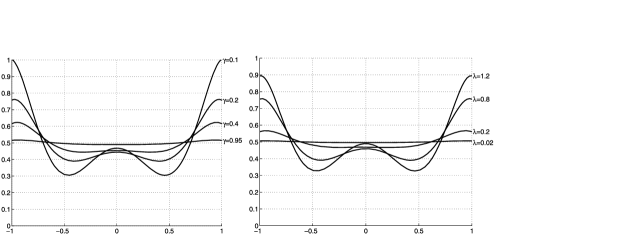
Figure 1: Asymptotic $D$-optimal design densities for least squares estimation in a random effect quadratic model for different choices of parameters in the covariance function (5) with $r(t)$ defined by (16). Right panel $\gamma=0.6$; left panel $\lambda=0.2$.

Further, we investigate the efficiency of an exact design derived from the asymptotic theory for least squares estimation, where the parameters in the correlation function (5) are given by

$$\quad\gamma=0.6,\qquad\sigma^{2}=0.5,\qquad V_{p}=\operatorname{diag}(\sigma_{\beta_{1}}^{2},\sigma_{\beta_{2}}^{2})=\operatorname{diag}(0.3^{2},0.3^{2}).$$ (17)

Let $\xi_{n}^{u}$ be an $n$-point equidistant design and $\xi_{n}^{a}$ be an $n$-point design obtained by the transformation (15) from the asymptotic optimal density. The points of the design $\xi_{n}^{a}$ and the exact optimal designs for least squares estimation for $\lambda=1.2$ are displayed in the left part of Figure 2. In the right part of Figure 2, we present the efficiencies for ordinary least squares estimation,

$$\operatorname{eff}_{\mathrm{OLS}}(\xi) = \biggl{(}{\det[(X^{T}X)^{-1}X^{T}V_{\varepsilon}X(X^{T}X)^{-1}+V_{p}]\over\det[(X^{T}_{\mathrm{OLS}}X_{\mathrm{OLS}})^{-1}X^{T}_{\mathrm{OLS}}V_{\varepsilon}X_{\mathrm{OLS}}(X^{T}_{\mathrm{OLS}}X_{\mathrm{OLS}})^{-1}+V_{p}]}\biggr{)}^{1/p},$$

and for weighted least squares estimation,

$$\operatorname{eff}_{\mathrm{WLS}}(\xi) = \biggl{(}{\det[X^{T}(V_{\varepsilon}+XV_{p}X^{T})^{-1}X]\over\det[X^{T}_{\mathrm{WLS}}(V_{\varepsilon}+X_{\mathrm{WLS}}V_{p}X^{T}_{\mathrm{WLS}})^{-1}X_{\mathrm{WLS}}]}\biggr{)}^{1/p}$$

for two designs: the design $\xi_{n}^{a}$, derived from asymptotic theory, and the uniform design $\xi_{n}^{u}$. Here $X$ denotes the design matrix obtained for the design $\xi$ under investigation, while $X_{\mathrm{OLS}}$ and $X_{\mathrm{WLS}}$ correspond to the optimal exact design for ordinary and weighted least squares estimation respectively. We observe that the design points concentrate in three regions containing the points of the exact $D$-optimal design for a quadratic regression with uncorrelated errors. It is also noteworthy that the designs derived from the asymptotic theory are very efficient, in particular, for weighted least squares estimation.

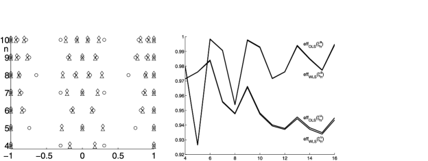
Figure 2: Left part: Various designs for ordinary and weighted least squares estimation in the random effect quadratic regression model. Exact $D$-optimal designs derived from asymptotic theory: ball; exact $D$-optimal for ordinary least squares estimation: diamond; exact $D$-optimal designs for weighted least squares estimation: triangle. Right part: Efficiency of the designs $\xi_{n}^{a}$ and equidistant design $\xi_{n}^{u}$ for ordinary and weighted least squares estimation. The parameters are given by (17), where $\lambda=1.2$.

4 Nonlinear random effect models

In this section we extend the methodology to the case of nonlinear random effect models, which have found considerable interest in the literature on pharmacokinetics. In this case, the results of experiments are modeled by

$$Y_{ij}=\eta(t_{j},b_{i})+\varepsilon_{ij},\qquad i=1,\ldots,K;j=1,\ldots,n.$$ (18)

Since the model (18) is nonlinear with respect to the variables $b_{i}$, there is no analytical expression for the likelihood function and various approximations have been considered in the literature [see Mentré, Mallet and Baccar (1997), Retout, Mentré and Bruno (2002), Retout and Mentré (2003), among others]. These approximations are used for the calculation of the maximum likelihood estimate and the corresponding Fisher information matrix. Alternatively, an estimate of the population mean $\beta$ can be obtained as an average of the nonlinear least squares estimates $\hat{b}_{i}$ for the different individuals, but due to the nonlinearity of the model, an explicit representation of the corresponding covariance matrix cannot be derived. Following Retout and Mentré (2003), we employ a first-order Taylor expansion to derive an approximation of this covariance matrix. To be precise, we obtain (under suitable assumptions of differentiability of the regression function) the approximation

$$\eta(t,b)\approx\eta(t,\beta)+g(t,\beta)(b-\beta)^{T},$$ (19)

where

$$g(t,b)=\frac{\partial\eta(t,b)}{\partial b}$$

denotes the gradient of the regression function with respect to $b$. This means that the nonlinear model (18) is approximated by the linear model (19). For the construction of the optimal design, we assume that knowledge about the parameter $\beta$ is available from previous or similar experiments. This corresponds to the concept of locally optimal designs, introduced by Chernoff (1953) in the context of fixed effect nonlinear regression models. Usually, locally optimal designs serve as benchmarks for commonly used designs and are the basis for the construction of optimal designs with respect to more sophisticated optimality criteria including the Bayesian and minimax approach [see Chaloner and Verdinelli (1995) or Dette (1995)].

Following the discussion in Section 3, we define the function $f(t,b)=g(t,b)/h(t)$ to account for heteroscedasticity. Note that the covariance matrix of the nonlinear least squares estimate in the model (18) is approximated by replacing the matrix $X$ in model (4) with $f(t)=f(t,b)|_{b=\beta}$, and the methodology described in Sections 2 and 3 can be applied to determine efficient designs. In the context of dose finding studies, it has been shown by means of a simulation study that the approximation (19) has sufficient accuracy for the construction of optimal designs [see Section 5 in Dette et al. (2008) for more details].

We further illustrate this concept by giving several examples for the case of homoscedastic errors. First, we investigate $D$- and $c$-optimal designs for the random effect model, which has recently been studied by Atkinson (2008). Next, we re-analyze the Uzara® and Lanicor® trials introduced in Section 1.

4.1 $D$-optimal design for a random effect compartmental model

We consider the random effect compartmental model with first-order absorption,

$$\eta(t,b)=\frac{b_{1}}{b_{1}-b_{2}}(e^{-b_{2}t}-e^{-b_{1}t}).$$ (20)

The model (20) is a special case of the Bateman function, defined in the introduction [see Garrett (1994)], and has found considerable attention in chemical sciences, toxicology and pharmacokinetics [see, e.g., Gibaldi and Perrier (1982)]. The optimal design problem in the compartmental fixed effect model has been studied by numerous authors [see, e.g., Box and Lucas (1959), Atkinson et al. (1993), Dette and O’Brien (1999), Biedermann, Dette and Pepelyshev (2004), among others], but much fewer results are available under the assumption of random effects. Recently optimal approximate designs for a random-effect compartmental model (20) have been determined by Atkinson (2008), but we did not find results about exact designs for these models in the presence of correlated errors. In the present paper we derive such designs from the asymptotic optimal design density and compare these designs with the exact optimal designs.

Note that the gradient of the function $\eta(t,b)$ with respect to $b$ is given by

$$g(t,b) = \biggl{(}\frac{b_{2}({e^{-b_{1}x}}-{e^{-b_{2}x}})+({b_{1}}^{2}x-b_{1}b_{2}x){e^{-b_{1}x}}}{(b_{1}-b_{2})^{2}},$$

$$\hskip 11.0pt\frac{b_{1}({e^{-b_{1}x}}-{e^{-b_{2}x}})+({b_{1}}^{2}x-b_{1}b_{2}x){e^{-b_{2}x}}}{(b_{1}-b_{2})^{2}}\biggr{)}^{T}.$$

In order to illustrate the methodology, we consider the same scenario as in Atkinson (2008) and assume that the parameters of the population and error distributions are the following: $\beta^{(0)}=(1,0.5)^{T}$,

$$\qquad\gamma=0.6,\qquad\sigma^{2}=0.01,\qquad V_{p}=\operatorname{diag}(\sigma_{\beta_{1}}^{2},\sigma_{\beta_{2}}^{2})=\operatorname{diag}(0.1^{2},0.05^{2}),$$ (22)

and the design space is given by the interval $T=[0,10]$. We assume that the function $r(t)$ in (5) is given by (16). The asymptotic $D$-optimal design densities for different values of the parameters are shown in Figure 3. We observe that, for $\gamma\to 1$ or $\lambda\to 0$, the $D$-optimal design densities approximate the uniform design, while, for larger values of $\lambda$ or small values of $\gamma$, the asymptotic $D$-optimal designs put more weight at two specific regions of the design space. This fact corresponds to intuition, because the (approximate) $D$-optimal design for the model (20) with uncorrelated observations is a two-point design [see, e.g., Box and Lucas (1959)].

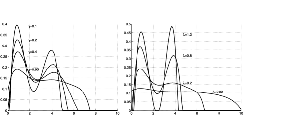
Figure 3: Asymptotic $D$-optimal design densities for nonlinear least squares estimation in the compartmental model (20) for different choices of the parameters in the covariance function (5) with $r(t)$ defined by (16). Left part: $\lambda=0.2$; right part: $\gamma=0.6$.

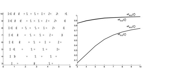
Figure 4: Left part: Various designs for ordinary and weighted nonlinear least squares estimation in the compartmental model (20). Exact $D$-optimal designs derived from asymptotic theory: ball; exact $D$-optimal for ordinary least squares estimation: diamond; exact $D$-optimal designs for weighted least squares estimation: triangle. Right part: Efficiency of the designs $\xi_{n}^{a}$ and $\xi_{n}^{u}$ for ordinary and weighted least squares estimation. The parameters are given by (22), where $\lambda=0.2$.

Further, we investigate the performance of the uniform and an exact design derived from asymptotic theory. For this purpose we define $\xi_{n}^{u}$ as an $n$-point equidistant design $\{10/n,20/n,\ldots,10\}$ and $\xi_{n}^{a}$ as the $n$-point design obtained by the transformation

$$t_{j}=(\Phi^{*})^{-1}\bigl{(}j/(n+1)\bigr{)},\qquad j=1,\ldots,n,$$

where $\Phi^{*}$ denotes the distribution function corresponding to the asymptotic $D$-optimal design density. Note this transformation is slightly different from the transformation (10) in order to exclude the point $0$ from the design points. Obviously, it is not reasonable to take observations $t=0$ in model (20), because it is assumed that the drug is administered at time $t=0$. The corresponding points of the exact designs are depicted in the left part of Figure 4, while the right part of the figure shows the $D$-efficiencies of the different designs. We observe that the designs derived from the asymptotic theory have a substantially larger $D$-efficiency compared to the uniform design. For example, for $n=6$, the $D$-efficiency of the uniform design is approximately $50\%$ for ordinary and weighted nonlinear least squares estimation, while the $D$-efficiency of the design $\xi_{n}^{a}$ is close to $90\%$.

It is worthwhile to mention that, in nonlinear random effect models, the optimal designs depend additionally on the mean $\beta$ of the distribution of the population parameters $b_{i}$. Therefore, it is of interest to investigate the sensitivity of the designs with respect to a misspecification of this parameter. For a study of the impact of such a misspecification on the efficiency of the resulting designs, we consider the case $n=4$ and $n=6$ and the corresponding designs $\xi^{a}_{4}=\{1.04,2.01,3.16,4.33\}$ and $\xi^{a}_{6}=\{0.83,1.47,2.32,3.30,4.20,5.20\}$, respectively. In Figure 5 we display the efficiencies

$$\hskip 19.0pt\biggl{(}{\det[(X^{T}X)^{-1}X^{T}V_{\varepsilon}X(X^{T}X)^{-1}+V_{p}]\over\det[(X^{T}_{\mathrm{OLS},\beta}X_{\mathrm{OLS},\beta})^{-1}X^{T}_{\mathrm{OLS},\beta}V_{\varepsilon}X_{\mathrm{OLS},\beta}(X^{T}_{\mathrm{OLS},\beta}X_{\mathrm{OLS},\beta})^{-1}+V_{p}]}\biggr{)}^{-1/p}$$ (23)

for different values of $\beta$. Here $X$ denotes the design matrix obtained from the design $\xi_{n}^{a}$ under the assumption that $\beta^{(0)}=(1,0,5)^{T}$, while the matrix $X_{\mathrm{OLS},\beta}$ corresponds to the exact $D$-optimal design for nonlinear least squares estimation for a specific $\beta$. The efficiencies are plotted in Figure 5 for the rectangle $[\beta_{i}^{(0)}-3\sigma_{\beta_{i}^{(0)}},\beta_{i}^{(0)}+3\sigma_{\beta_{i}^{(0)}}]=[0.7,1.3]\times[0.35,0.65]$. It can be seen that the exact optimal design, derived from the asymptotic theory, has a high $D$-efficiency with respect to misspecification of the population mean $\beta$ over a broad range.

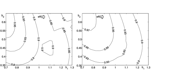
Figure 5: $D$-efficiencies of the designs $\xi^{a}_{4}=\{1.04,2.01,3.16,4.33\}$ (left part) and the design $\xi^{a}_{6}=\{0.83,1.47,2.32,3.30,4.20,5.20\}$ (right part) (these designs are obtained from asymptotic density) for nonlinear least squares estimation in the random effect compartmental model (20), if the mean of the population distribution has been misspecified. The parameters of the population distribution are given by (22) with $\lambda=0.2$.

4.2 Optimal designs for estimating the AUC

In some bioavailability studies, the aim of experiments is the estimation of the area under curve

$$\mathrm{AUC}=\int_{0}^{\infty}\eta(t,\beta)\,dt.$$

For the compartmental model (20), we obtain $\mathrm{AUC}={1}/{b_{2}}$. It can be shown that the locally AUC-optimal design for model (20) minimizes the variance of the nonlinear least squares estimate for the parameter $\beta_{2}$. This variance is approximately proportional to

$$(0,1)\bigl{(}(X^{T}X)^{-1}X^{T}V_{\varepsilon}X(X^{T}X)^{-1}+V_{p}\bigr{)}(0,1)^{T}.$$

This expression corresponds to the $c$-optimality criterion, which has been discussed extensively in the literature for fixed effect models with uncorrelated observations [see, e.g., Ford, Torsney and Wu (1992), Fan and Chaloner (2003) and Dette et al. (2008), among others]. The asymptotic optimal design densities for estimating the area under the curve are shown in Figure 6. We observe again that the optimal density is close to the uniform design density if $\lambda\to 0$ or $\gamma\to 1$. On the other hand, if $\lambda$ is large or $\gamma\to 0$, the AUC-optimal design density has a narrow support. This fact reflects that the optimal design for estimating the area under the curve in the fixed effect compartmental model with uncorrelated observations is a one-point design. In Figure 7 we show the designs derived from the asymptotic optimal design densities, and the exact optimal designs for estimating the area under the curve in the compartmental model. We observe that the designs $\xi^{a}_{n}$, derived from the asymptotic optimal design density, are very close to the exact optimal designs for least squares estimation of the area under the curve. Moreover, the design $\xi_{n}^{a}$ yields a substantial improvement in efficiency compared to the uniform design. Again we observe that the designs derived for ordinary least squares estimation also have excellent efficiencies for weighted least squares estimation of the AUC (see the right part of Figure 7).

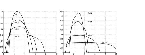
Figure 6: Asymptotic optimal densities for estimating the area under the curve in the compartmental model (20) for different choices of the parameters in the covariance function (5) with $r(t)$ defined by (16). Left part: $\lambda=0.2$, right part: $\gamma=0.6$.

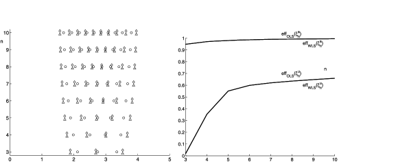
Figure 7: Left part: Various designs for estimating the area under the curve in the compartmental model (20). Designs derived from asymptotic theory: ball; exact optimal designs for least squares estimation of the area under the curve: diamond; exact optimal designs for weighted least squares estimation: triangle. Right part: Efficiency of the designs $\xi_{n}^{a}$ and $\xi_{n}^{u}$ for ordinary and weighted least squares estimation of the AUC. The parameters are given by (22), where $\lambda=1.2$.

4.3 Optimal designs for estimating the AUC in the Uzara® and Lanicor® trials

In this section we consider the optimal design problem for estimating the AUC in the two examples presented in the introduction. The medical background of these examples was a small pilot trial of 4 patients [Thürmann, Neff and Fleisch (2004)], where it was observed that patients taking the over-the-counter herbal diarrhea medication Uzara® (in the form of drops, i.e., oral application) showed high values in medical assays designed to measure the blood serum concentration of digitoxin, a potent treatment against heart insufficiency. This is caused by the chemical similarity of these two substances and can result in major complications in establishing treatment programs for heart insufficiency. It was thus decided to compare the pharmacokinetic properties of an oral application of Uzara® to the properties of the usual intravenous application of a regular digitoxin medication (Lanicor®) on a larger sample size of 18 patients, with 15 measurements each. The main focus of the comparison was the area under the concentration curve as a measure of the total effect of an application. A preliminary design was proposed by experts in order to allow precise estimation of this property, and the study was carried out according to this design. We will now investigate the efficiency of this and a naively chosen equally spaced design compared to a design generated using the methods presented in this paper.

In order to compute the design densities, it is necessary to estimate the parameters for both of the models. To do so, we used the full 18 patient data set, however, this could have been done as well using only the 4 patients of the pilot study. We estimated parameters using a combination of maximum likelihood and least squares techniques [see Pinheiro and Bates (1995)]. For the intravenous part corresponding to model (1), we have received the estimates $\hat{\beta}=(30,0.75)^{T}$,

$$\hat{V}_{p}=\pmatrix{9&0.189\vspace*{2pt}\cr 0.189&0.0049}$$

for the population parameters, while the estimates of the parameters in the covariance matrix (3) are given by $\hat{\gamma}=0.8$, $\hat{\lambda}=0.05$, $\hat{\sigma}^{2}=0.6$.

For the oral application corresponding to model (2), the estimates of the parameters are given by $\hat{\beta}=(0.2,0.135,28)^{T}$,

$$\hat{V}_{p}=\pmatrix{0.0025&0.0019&0\vspace*{2pt}\cr 0.0019&0.0016&0\vspace*{2pt}\cr 0&0&144}$$

and $\hat{\gamma}=0.8$, $\hat{\lambda}=0.01$, $\hat{\sigma}^{2}=0.2$. Note that the entries in the positions $(1,3)$, $(2,3)$, $(3,1)$ and $(3,2)$ are not identical $0$, but smaller than $10^{-5}$. Based on a preliminary discussion with experts, the physicians decided to take measurements for both experiments at nearly identical (nonoptimized) time points

$$0,0.5,1,1.5,2,3,4,5,6,8,10,12,15,24,36$$

and

$$0.25,0.75,1.25,2,3,4,5,6,8,10,12,15,24,36,$$

respectively. Note that in the second design an additional measurement was taken at $t=-0.25$, that is, before the intravenous injection. Since this point is out of the scope of the exponential evasion model, the observation at this time has been excluded from further considerations. Thus, the Lanicor® trial has $n=14$ observations.

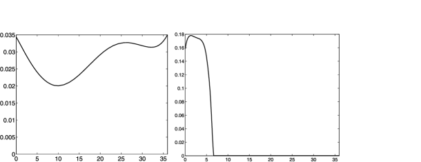
Figure 8: Asymptotic optimal density for estimating the area under the curve in the $3$-parameter Bateman (left part) and exponential evasion model (right part).

For the estimated parameters, we have derived the asymptotic optimal design densities, which are depicted in the left and right part of Figure 8 for the Uzara® and Lanicor® trials, respectively, where the design interval is given by $T=[0,36]$. The resulting designs from these densities are given by

$$2.09,4.55,7.49,10.8,13.9,16.8,19.2,21.5,23.6,25.7,27.7,29.8,31.9,34.0,36$$

for the Uzara® trial and

$$0.432,0.85,1.25,1.66,2.06,2.46,2.87,3.28,3.7,4.12,4.55,5.01,5.54,36$$

for the Lanicor® trial. This means that the asymptotic optimal design for the oral application is close to an equally spaced design, while the optimal design for the intravenous application is much more focused on measurements at early time points. This result is plausible in an exponential elimination model. Calculating the efficiencies for ordinary least squares estimation of these asymptotic optimal designs compared to the exact optimal design, we obtain efficiencies $0.99$ and $0.95$, respectively, indicating that these designs are quite good.

Upon numerical studies, we can further conclude that the constructed designs are robust to misspecification of the initial guess of parameters. For example, variations of $\lambda$ (or any of the other parameters) by up to 50% yield a drop of efficiency by less than $0.02$.

Note that in the examples presented in Sections 3, 4.1 and 4.2, the efficiencies of the derived designs for weighted least squares estimation are very similar to the efficiencies for ordinary least squares estimation, and a similar observation has been made for the two trials under investigation. The efficiencies for weighted least squares estimation of the designs based on the asymptotic density are 99% (Uzara®) and 97% (Lanicor®), even better than the efficiencies for ordinary least squares estimation.

We now investigate the performance of the designs which were actually used in the clinical trial. We found that these designs have efficiency $0.96$ and $0.92$ for estimating the AUC through OLS estimation in the Uzara® and Lanicor® trials, respectively. Thus, the preliminary designs, recommended by experts, are rather efficient in both trials.

Let us now investigate the performance of naively chosen equidistant designs: the design

$$0,2.6,5.1,7.7,10.3,12.8,15.4,18.0,20.6,23.1,25.7,28.3,30.8,33.4,36$$

for the Uzara® trial, and the design

$$0,2.8,5.5,8.3,11.1,13.9,16.6,19.4,22.2,24.9,27.7,30.5,33.2,36$$

for the Lanicor® trial. Comparing these designs to the optimal designs, we obtain efficiencies of $0.97$ and $0.41$ for ordinary least squares estimation of the AUC in the Uzara® and Lanicor® trials, respectively.

It was pointed out by a referee that it is of some interest to investigate the performance of the optimal designs proposed in this paper for the estimation of the variance of the random effects (i.e., the parameters of the matrix $V_{p}$). These parameters are usually estimated by maximum likelihood techniques [see Retout and Mentré (2003), among others] and the corresponding information matrix of these estimates is of a fundamentally different structure compared to the variance matrix of the least squares estimate. For the two optimal designs we have calculated the $D$-efficiencies for estimating the diagonal elements of the matrix $V_{p}$, which are $96$% and $79$% in the Uzara® and Lanicor® trial, respectively. The designs actually used in the trial have efficiency $98\%$ and $85\%$, while the corresponding efficiencies of the uniform designs are $98\%$ and $63\%$, respectively. Thus, the proposed optimal designs for AUC-estimation also have reasonable efficiency for estimation of the covariance matrix of the population distribution.

Summarizing the discussion in this example, we conclude that the equally spaced design in the Uzara® trial is very close to the optimal design determined by the proposed methodology, and it is for this reason very efficient. However, the equally-spaced designs do not always have high efficiency. In the Lanicor® trial, the use of naively chosen designs yields considerably less accurate estimates. For this reason, the application of experimental design techniques in the context of pharmacokinetics trials is strictly recommended.

References

- Aarons (1999) Aarons, L. (1999). Software for population pharmacokinetics and pharmacodynamics. Clinical Pharmacokinetics 36 255–264.
- Atkinson (2008) Atkinson, A. C. (2008). Examples of the use of an equivalence theorem in constructing optimum experimental designs for random-effects nonlinear regression models. J. Statist. Plann. Inference 138 2595–2606. \MR2439971
- Atkinson and Donev (1992) Atkinson, A. C. and Donev, A. (1992). Optimum Experimental Designs. Clarendon Press, Oxford.
- Atkinson et al. (1993) Atkinson, A. C., Chaloner, K., Herzberg, A. M. and Juritz, J. (1993). Optimum experimental designs for properties of a compartmental model. Biometrics 49 325–337.
- Bickel and Herzberg (1979) Bickel, P. J. and Herzberg, A. M. (1979). Robustness of design against autocorrelation in time I: Asymptotic theory, optimality for location and linear regression. Ann. Statist. 7 77–95. \MR0515685
- Bickel, Herzberg and Schilling (1981) Bickel, P. J., Herzberg, A. M. and Schilling, M. F. (1981). Robustness of design against autocorrelation in time II: Optimality, theoretical and numerical results for the first-order autoregressive process. J. Amer. Statist. Assoc. 76 870–877. \MR0650898
- Biedermann, Dette and Pepelyshev (2004) Biedermann, S., Dette, H. and Pepelyshev, A. (2004). Maximin optimal designs for a compartmental model. In MODA 7—Advances in Model-Oriented Design and Analysis 41–48. Physica-Verlag, Heidelberg. \MR2089324
- Box and Lucas (1959) Box, G. E. P. and Lucas, H. L. (1959). Design of experiments in non-linear situations. Biometrika 46 77–90. \MR0102155
- Buelga et al. (2005) Buelga, D. S., del Mar Fernandez de Gatta, M., Herrera, E. V., Dominguez-Gil, A. and Garcia, M. J. (2005). The Bateman function revisited: A critical reevaluation of the quantitative expressions to characterize concentrations in the one compartment body model as a function of time with first-order invasion and first-order elimination. Antimicrobial Agents and Chemotherapy 49 103–128.
- Chaloner and Verdinelli (1995) Chaloner, K. and Verdinelli, I. (1995). Bayesian experimental design: A review. Statist. Sci. 10 237–304. \MR1390519
- Chernoff (1953) Chernoff, H. (1953). Locally optimal designs for estimating parameters. Ann. Math. Statist. 24 586–602. \MR0058932
- Colombo et al. (2006) Colombo, S., Buclin, T., Cavassini, M., Decosterd, L., Telenti, A., Biollaz, J. and Csajka, C. (2006). Population pharmacokinetics of atazanavir in patients with human immunodeficiency virus infection. Antimicrobial Agents and Chemotherapy 50 3801–3808.
- Dette (1995) Dette, H. (1995). Designing of experiments with respect to “standardized” optimality criteria. J. Roy. Statist. Soc. Ser. B 59 97–110. \MR1436556
- Dette and O’Brien (1999) Dette, H. and O’Brien, T. (1999). Optimality criteria for regression models based on predicted variance. Biometrika 86 93–106. \MR1688074
- Dette et al. (2008) Dette, H., Bretz, F., Pepelyshev, A. and Pinheiro, J. C. (2008). Optimal designs for dose finding studies. J. Amer. Statist. Assoc. 103 1225–1237. \MR2462895
- Fan and Chaloner (2003) Fan, S. K. and Chaloner, K. (2003). A geometric method for singular -optimal designs. J. Statist. Plann. Inference 113 249–257. \MR1963044
- Fedorov (1972) Fedorov, V. V. (1972). Theory of Optimal Experiments. Academic Press, New York. \MR0403103
- Fedorov and Hackl (1997) Fedorov, V. V. and Hackl, P. (1997). Model-Oriented Design of Experiments. Lecture Notes in Statist. 125. Springer, New York. \MR1454123
- Ford, Torsney and Wu (1992) Ford, I., Torsney, B. and Wu, C. F. J. (1992). The use of canonical form in the construction of locally optimum designs for nonlinear problems. J. Roy. Statist. Soc. Ser. B 54 569–583. \MR1160483
- Gaffke and Krafft (1982) Gaffke, N. and Krafft, O. (1982). Exact -optimum designs for quadratic regression. J. Roy. Statist. Soc. Ser. B 44 394–397. \MR0693239
- Garrett (1994) Garrett, E. R. (1994). The Bateman function revisited: A critical reevaluation of the quantitative expressions to characterize concentrations in the one compartment body model as a function of time with first-order invasion and first-order elimination. Journal of Pharmacokinetics and Biopharmaceutics 22 103–128.
- Gibaldi and Perrier (1982) Gibaldi, M. and Perrier, D. (1982). Parmacokinetics, 2nd ed. Dekker, New York.
- Harville (1976) Harville, D. (1976). Extension of the Gauss–Markov theorem to include the estimation of random effects. Ann. Statist. 4 384–395. \MR0398007
- Mentré, Mallet and Baccar (1997) Mentré, F., Mallet, A. and Baccar, D. (1997). Optimal design in random-effects regression models. Biometrika 84 429–442. \MR1467058
- Pázman (1986) Pázman, A. (1986). Foundations of Optimum Experimental Design. D. Reidel, Dordrecht. \MR0838958
- Pinheiro and Bates (1995) Pinheiro, J. C. and Bates, D. M. (1995). Approximations to the log-likelihood function in the nonlinear mixed effects model. J. Comput. Graph. Statist. 4 12–35.
- Pukelsheim (1993) Pukelsheim, F. (1993). Optimal Design of Experiments. Wiley, New York. \MR1211416
- Retout and Mentré (2003) Retout, S. and Mentré, F. (2003). Further developments of the Fisher information matrix in nonlinear mixed-effects models with evaluation in population pharmacokinetics. Journal of Biopharmaceutical Statistics 13 209–227.
- Retout, Duffull and Mentre (2001) Retout, S., Duffull, S. and Mentre, F. (2001). Development and implementation of the Fisher information matrix for the evaluation of population pharmakokinetic designs. Computer Methods and Programs in Biomedicine 65 141–151.
- Retout, Mentré and Bruno (2002) Retout, S., Mentré, F. and Bruno, R. (2002). Fisher information matrix for nonlinear mixed-effects models: Evaluation and application for optimal design of enoxaparin population pharmacokinetics. Stat. Med. 21 2623–2639.
- Sacks and Ylvisaker (1966) Sacks, J. and Ylvisaker, N. D. (1966). Designs for regression problems with correlated errors. Ann. Math. Statist. 37 66–89. \MR0192601
- Sacks and Ylvisaker (1968) Sacks, J. and Ylvisaker, N. D. (1968). Designs for regression problems with correlated errors; many parameters. Ann. Math. Statist. 39 49–69. \MR0220424
- Schmelter (2007a) Schmelter, T. (2007a). Considerations on group-wise identical designs for linear mixed models. J. Statist. Plann. Inference 137 4003–4010. \MR2368544
- Schmelter (2007b) Schmelter, T. (2007b). The optimality of single-group designs for certain mixed models. Metrika 65 183–193. \MR2288057
- Shargel (1993) Shargel, L. (1993). Applied Biopharmaceutics and Pharmacokinetics. Chapman & Hall, London.
- Silvey (1980) Silvey, S. D. (1980). Optimal Design. Chapman & Hall, London. \MR0606742
- Thürmann, Neff and Fleisch (2004) Thürmann, P., Neff, A. and Fleisch, J. (2004). Interference of Uzara glycosides in assays of digitalis glycosides. International Journal of Clinical Pharmacology and Therapeutics 42 281–284.