The greatest convex minorant of Brownian motion, meander, and bridge

Abstract

This article contains both a point process and a sequential description of the greatest convex minorant of Brownian motion on a finite interval. We use these descriptions to provide new analysis of various features of the convex minorant such as the set of times where the Brownian motion meets its minorant. The equivalence of the these descriptions is non-trivial, which leads to many interesting identities between quantities derived from our analysis. The sequential description can be viewed as a Markov chain for which we derive some fundamental properties.

1 Introduction

The greatest convex minorant (or simply convex minorant for short) of a real-valued function $(x_{u},u\in U)$ with domain $U$ contained in the real line is the maximal convex function $(\underline{c}_{u},u\in I)$ defined on a closed interval $I$ containing $U$ with $\underline{c}_{u}\leq x_{u}$ for all $u\in U$. A number of authors have provided descriptions of certain features of the convex minorant for various stochastic processes such as random walks [17], Brownian motion [9, 11, 19, 25, 28], Cauchy processes [6], Markov Processes [4], and Lévy processes (Chapter XI of [23]).

In this article, we will give two descriptions of the convex minorant of various Brownian path fragments which yield new insight into the structure of the convex minorant of a Brownian motion over a finite interval. As we shall see below, such a convex minorant is a piecewise linear function with infinitely many linear segments which accumulate only at the endpoints of the interval. We refer to linear segments as “faces,” the “length” of a face is as projected onto the horizontal time axis, and the slope of a face is the slope of the corresponding segment. We also refer to the points where the convex minorant equals the process as vertices; note that these points are also the endpoints of the linear segments. See figure 1 for illustration.

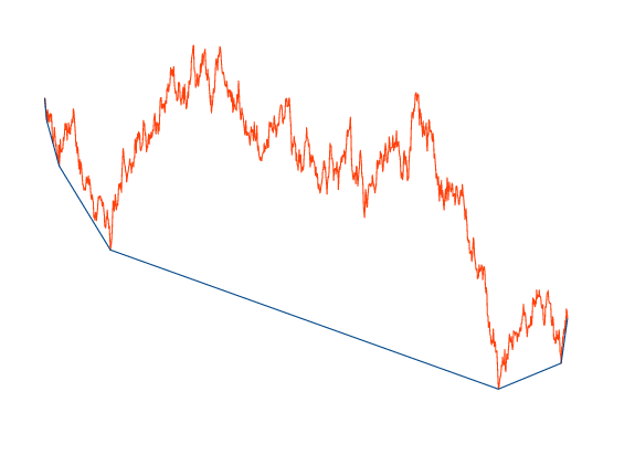
Figure 1: A typical instance of a finite time Brownian motion and its convex minorant. The “faces” of the convex minorant are the linear segments, the “lengths” are as projected to a horizontal axis, and the “slope” is the slope of the segment.

Our first description is a Poisson point process of the lengths and slopes of the faces of the convex minorant of Brownian motion on an interval of a random exponential length. This result can be derived from the recent developments of [2] and [27] and is in the spirit of previous studies of the convex minorant of Brownian motion run to infinity (e.g. [19]). We provide a proof below in Section 3.

Theorem 1.

Let $\Gamma_{1}$ an exponential random variable with rate one. The lengths $x$ and slopes $s$ of the faces of the convex minorant of a Brownian motion on $[0,\Gamma_{1}]$ form a Poisson point process on $\mathbb{R}^{+}\times\mathbb{R}$ with intensity measure

$$\frac{\exp\{-\frac{x}{2}\left(2+s^{2}\right)\}}{\sqrt{2\pi x}}\,ds\,dx,\hskip 14.22636ptx\geq 0,s\in\mathbb{R}.$$ (1)

We will pay special attention to the set of times of the vertices of the convex minorant of a Brownian motion on $[0,1]$. To this end, let

$$0<\cdots<\alpha_{-2}<\alpha_{-1}<\alpha_{0}<\alpha_{1}<\alpha_{2}<\cdots<1$$ (2)

with $\alpha_{-n}\downarrow 0$ and $\alpha_{n}\uparrow 1$ as $n\rightarrow\infty$ denote the times of vertices of the convex minorant of a Brownian motion $B$ on $[0,1]$, arranged relative to

$$\alpha_{0}:={\rm argmin}_{0\leq t\leq 1}B_{t}.$$ (3)

Theorem 1 implicitly contains the distribution of the sequence $(\alpha_{i})_{i\in\mathbb{Z}}$. This description is precisely stated in the following corollary of Theorem 1, which follows easily from Brownian scaling.

Corollary 2.

If $\{(L_{i},S_{i}),i\in\mathbb{Z}\}$ are the lengths and slopes given by the Poisson point process with intensity measure (1), arranged so that

$$\cdots S_{-1}<S_{0}<0<S_{1}<S_{2}\cdots$$

then

$$\left(\alpha_{n}\right)_{n\in\mathbb{Z}}\mbox{$\ \stackrel{{\scriptstyle d}}{{=}}$ }\left(\sum_{i\leq n}L_{i}\bigg{/}\sum_{i\in\mathbb{Z}}L_{i}\right)_{n\in\mathbb{Z}}.$$

Our second description provides a Markovian recursion for the vertices of the convex minorant of a Brownian meander (and Bessel(3) process and bridge), which applies to Brownian motion on a finite interval through Denisov’s decomposition at the minimum [12] - background on these concepts is provided in Section 2. In our setting, Denisov’s decomposition of Brownian motion on $[0,1]$ states that conditional on $\alpha_{0}$, the pre and post minimum processes are independent Brownian meanders of appropriate lengths. We now make the following definition.

Definition 3.

We say that a sequence of random variables $(\tau_{n},\rho_{n})_{n\geq 0}$ satisfies the $(\tau,\rho)$ recursion if for all $n\geq 0$:

$$\rho_{n+1}=U_{n}\rho_{n}$$

and

$$\tau_{n+1}=\frac{\tau_{n}\rho_{n+1}^{2}}{\tau_{n}Z_{n+1}^{2}+\rho_{n+1}^{2}}$$

for the two independent sequences of i.i.d. uniform $(0,1)$ variables $U_{n}$ and i.i.d. squares of standard normal random variables $Z_{n}^{2}$, both independent of $(\tau_{0},\rho_{0})$.

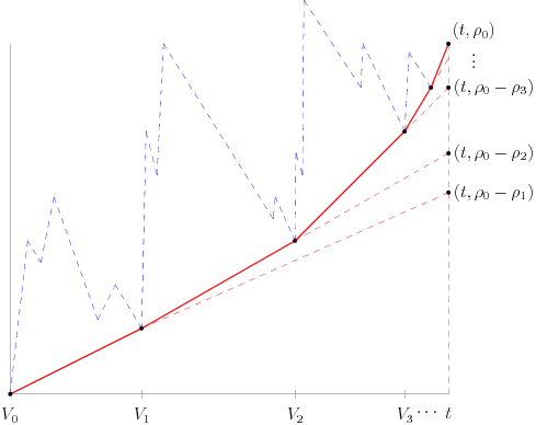
Figure 2: An illustration of the notation of Theorem 4. The dashed line represents a Brownian meander of length $t$, and the solid line its convex minorant. Note also that $V_{i}:=t-\tau_{i}$ for $i=0,1,\ldots$

Theorem 4.

Let $(X(v),0\leq v\leq t)$ be a Brownian meander of length $t$, and let $(\underline{C}(v),0\leq v\leq t)$ be its convex minorant. The vertices of $(\underline{C}(v),0\leq v\leq t)$ occur at times $0=V_{0}<V_{1}<V_{2}<\cdots$ with $\lim_{n}V_{n}=t$. Let $\tau_{n}:=t-V_{n}$ so $\tau_{0}=t>\tau_{1}>\tau_{2}>\cdots$ with $\lim_{n}\tau_{n}=0$. Let $\rho_{0}=X(t)$ and for $n\geq 1$ let $\rho_{0}-\rho_{n}$ denote the intercept at time $t$ of the line extending the segment of the convex minorant of $X$ on the interval $(V_{n-1},V_{n})$. The convex minorant $\underline{C}$ of $X$ is uniquely determined by the sequence of pairs $(\tau_{n},\rho_{n})$ for $n=1,2,\ldots$ which satisfies the $(\tau,\rho)$ recursion with

$$\rho_{0}\mbox{$\ \stackrel{{\scriptstyle d}}{{=}}$ }\sqrt{2t\Gamma_{1}}\mbox{ and }\tau_{0}=t,$$ (4)

where $\Gamma_{1}$ is an exponential random variable with rate one.

Once again, Theorem 4 implicitly contains the distribution of the sequence $(\alpha_{i})_{i\in\mathbb{Z}}$, as described in the following corollary which follows from Denisov’s decomposition and Brownian scaling.

Corollary 5.

Let $0=1-\tau_{0}<1-\tau_{1}<\cdots$ and $0=1-{\hat{\tau}}_{0}<1-{\hat{\tau}}_{1}<\cdots$ be the times of the vertices of the convex minorants of two independent and identically distributed standard Brownian meanders. Then the sequence $(\alpha_{i})_{i\in\mathbb{Z}}$ of times of vertices of the convex minorant of Brownian motion on $[0,1]$ may be represented for $n\geq 0$ as

$$\alpha_{-n} =\tau_{n}\alpha_{0},\,$$

$$\alpha_{n} =1-{\hat{\tau}}_{n}(1-\alpha_{0})\mbox{$\ \stackrel{{\scriptstyle d}}{{=}}$ }1-\alpha_{-n},$$

where $\alpha_{0}$ is independent of the sequences $(\tau_{i})_{i\geq 0}$ and $({\hat{\tau}}_{i})_{i\geq 0}$.

Corollaries 2 and 5 provide a bridge between the two descriptions of Theorems 1 and 4 so that each of these descriptions is implied by the other. More precisely, we have the following (Brownian free) formulation, where here and below for $s>0$, $\Gamma_{s}$ denotes a gamma random variable with density

$$\frac{x^{s-1}e^{-x}}{\Gamma(s)},\hskip 14.22636ptx>0,$$

and where $\Gamma(s)$ denotes the gamma function.

Theorem 6.

If the sequence of random variables $(\tau_{n},\rho_{n})_{n\geq 0}$ satisfies the $(\tau,\rho)$ recursion with

$$\tau_{0}\mbox{$\ \stackrel{{\scriptstyle d}}{{=}}$ }\Gamma_{1/2},\hskip 17.07164pt\rho_{0}\mbox{$\ \stackrel{{\scriptstyle d}}{{=}}$ }\sqrt{2\Gamma_{1/2}\Gamma_{1}},$$ (5)

where $\Gamma_{1/2}$ and $\Gamma_{1}$ are independent, then the random set of pairs

$$\left\{\left(\tau_{i-1}-\tau_{i},\sum_{j=1}^{i}\frac{\rho_{j-1}-\rho_{j}}{\tau_{j-1}}\right):i\in\mathbb{N}\right\}$$

forms a Poisson point process on $\mathbb{R}^{+}\times\mathbb{R}^{+}$ with intensity measure

$$\frac{\exp\{-\frac{x}{2}\left(2+s^{2}\right)\}}{\sqrt{2\pi x}}\,ds\,dx,\hskip 14.22636ptx,s\geq 0.$$ (6)

Conversely, if $\{(L_{i},S_{i}):i\in\mathbb{N}\}$ is the set of points of a Poisson point process with intensity measure given by (6), ordered so that $S_{0}:=0<S_{1}<S_{2}<\ldots$ then the variables

$$\tau_{i}=\sum_{j=i+1}^{\infty}L_{j}\mbox{\,\, \rm{and} \,\,}\rho_{i}=\sum_{j=i+1}^{\infty}S_{j}L_{j}-S_{i}\sum_{j=i+1}^{\infty}L_{j},\,\,i=0,1,2,\ldots$$

satisfy the $(\tau,\rho)$ recursion with $(\tau_{0},\rho_{0})$ distributed as in (5).

Proof.

The theorem is proved by Brownian scaling in the relevant facts above coupled with the fundamental identity $\alpha_{0}\Gamma_{1}\mbox{$\ \stackrel{{\scriptstyle d}}{{=}}$ }\Gamma_{1/2}$, where $\alpha_{0}$ and $\Gamma_{1}$ are independent.  

It is not at all obvious how to show Theorem 6 directly. Moreover, many simple quantities can be computed and related to both descriptions which we cannot independently show to be equivalent. For example, we have the following result which follows from Theorem 6, but for which we do not have an independent proof - see Section 5 below.

Corollary 7.

Let $W$ and $Z$ standard normal random variables, $U$ uniform on $(0,1)$, and $R$ Rayleigh distributed having density $re^{-r^{2}/2}$, $r>0$. If all of these variables are independent, then

$$\frac{W^{2}+(1-U)^{2}R^{2}}{1+U^{2}R^{2}/Z^{2}}\mbox{$\ \stackrel{{\scriptstyle d}}{{=}}$ }Z^{2}.$$

The layout of the paper is as follows. Section 2 contains the notation and much of the background used in the paper. Sections 3 and 4 respectively contain the Poisson and sequential descriptions of the convex minorant of various Brownian paths and in Section 5 we discuss identities derived by relating the two descriptions. In Section 6 we derive various densities and transforms associated to the process of vertices and slopes of faces of the convex minorant and in Section 7 we discuss some aspects (including a CLT) of the Markov process implicit in the sequential construction.

2 Background

This section recalls some background and terminology for handling various Brownian path fragments.

Let $(B(t),t\geq 0)$ denote a standard one-dimensional Brownian motion, abbreviated $BM^{0}$, and let $(R_{3}(t),t\geq 0)$ denote a standard 3-dimensional Bessel process, abbreviated $BES^{0}(3)$, defined as the square root of the sum of squares of $3$ independent copies of $B$. So $B(0)=R_{3}(0)=0$, $E(B(t)^{2})=t$ and $E(R_{3}(t)^{2})=3t$. The notation $BM^{x}$ and $BES^{x}(3)$ will be used to denote these processes with a general initial value $x$ instead of $x=0$, where necessarily $x\geq 0$ for $BES^{x}(3)$.

Bridges

For $0\leq s<t$ and real numbers $x$ and $y$, a Brownian bridge from $(s,x)$ to $(t,y)$ is a process identical in law to $(B(u),s\leq u\leq t)$ given $B(s)=x$ and $B(t)=y$, constructed to be weakly continuous in $x$ and $y$ for fixed $s$ and $t$. The explicit construction of all such bridges by suitable scaling of the standard Brownian bridge from $(0,0)$ to $(1,0)$ is well known, as is the fact that for $B$ a $BM^{0}$ the process

$$(B(t)-tB(1),0\leq t\leq 1)$$

is a standard Brownian bridge independent of $B(1)$.

The family of $BES(3)$ bridges from $(s,x)$ to $(t,y)$ is defined similarly for $0\leq s<t$ and $x,y\geq 0$. The $BES(3)$ bridge from $(s,x)$ to $(t,y)$ is a Brownian bridge from $(s,x)$ to $(t,y)$ conditioned to remain strictly positive on $(s,t)$. For $x>0$ and $y>0$ the conditioning event for the Brownian bridge has a strictly positive probability, so the conditioning is elementary, and the assertion is easily verified. If either $x=0$ or $y=0$ the conditioning event has zero probability, and the assertion can either be interpreted in terms of weak limits as either $x$ or $y$ or both approach $0$, or in terms of $h$-processes [8, 10, 14].

Excursions and meanders

The $BES(3)$ bridge from $(0,0)$ to $(t,0)$ is known as a Brownian excursion of length $t$. This process can be constructed by Brownian scaling as $(\sqrt{t}B^{\mbox{$\scriptstyle{\rm ex}$}}(v/t),0\leq v\leq t)$ where $(B^{\mbox{$\scriptstyle{\rm ex}$}}(u),0\leq u\leq 1)$ is the standard Brownian excursion of length $1$. Intuitively, the Brownian excursion of length $t$ should be understood as $(B(v),0\leq v\leq t)$ conditioned on $B(0)=B(t)=0$ and $B(v)>0$ for all $0<v<t$. Similarly, conditioning $(B(v),0\leq v\leq t)$ on $B(0)=0$ and $B(v)>0$ for all $0<v<t$, without specifying a value for $B(t)$, leads to the concept of a Brownian meander of length $t$. This process can be constructed as $(\sqrt{t}B^{\mbox{$\scriptstyle{\rm me}$}}(v/t),0\leq v\leq t)$ where $(B^{\mbox{$\scriptstyle{\rm me}$}}(u),0\leq u\leq 1)$ is the standard Brownian meander of length $1$ which for our purposes is best considered via the following result of Imhof [20].

Proposition 8.

[20] If $(R_{3}(t),0\leq t\leq 1)$ is a $BES^{0}(3)$ process, then the process $(B^{\mbox{$\scriptstyle{\rm me}$}}(u),0\leq u\leq 1)$ is absolutely continuous with respect to the law of $(R_{3}(t),0\leq t\leq 1)$, with density $(\pi/2)^{1/2}x^{-1}$, where $x=R_{3}(1)$ is the final value of $R_{3}$ . Thus, $R_{3}$ and $B^{\mbox{$\scriptstyle{\rm me}$}}$ share the same collection of $BES(3)$ bridges from $(0,0)$ to $(1,r)$ obtained by conditioning on the final value $r$.

We also say $(X(t),0\leq t\leq T)$ is a Brownian meander of random length $T>0$, if $(T^{-1/2}X(uT),0\leq u\leq 1)\mbox{$\ \stackrel{{\scriptstyle d}}{{=}}$ }(B^{\mbox{$\scriptstyle{\rm me}$}}(u),0\leq u\leq 1)$, with $B^{\mbox{$\scriptstyle{\rm me}$}}$ independent of $T$. Informally, $X$ is a random path of random length. Formally, we may represent $X$ as a random element of $C[0,\infty)$ by stopping the path at time $T$.

We recall the following basic path decomposition for standard Brownian motion run for a finite time due to Denisov [12]. Recall that the Rayleigh distribution has density $re^{-r^{2}/2}$ for $r>0$, and the arcsine distribution has density $1/(\pi\sqrt{x(1-x)})$ on $[0,1]$.

Proposition 9.

[12](Denisov’s Decomposition). Let $(B(u),u\geq 0)$ be a Brownian motion, and let $T$ be the a.s. unique time that $B$ attains its minimum on $[0,1]$ and $M=B(T)$ its minimum.

• $(T,M)\mbox{$\ \stackrel{{\scriptstyle d}}{{=}}$ }(\beta,-\sqrt{\beta}R)$, where $\beta$ has the arcsine distribution, $R$ has the Rayleigh distribution, and $\beta$ and $R$ are independent.

• Given $T$, the processes $(B(T-u)-M,0\leq u\leq T)$ and $(B(T+u)-M,0\leq u\leq 1-T)$ are independent Brownian meanders of lengths $T$ and $1-T$, respectively.

We will frequently use variations of this result derived by Brownian scaling and conditioning; for example we have the following proposition, which can be viewed as a formulation of Williams decomposition [29].

Proposition 10.

Let $(B(u),u\geq 0)$ be a Brownian motion and $\Gamma_{1}$ an exponential random variable with rate one independent of $B$. Let $T$ be the a.s. unique time that $B$ obtains its minimum on $[0,\Gamma_{1}]$, and $M=B(T)$ its minimum.

• $(T,M)\mbox{$\ \stackrel{{\scriptstyle d}}{{=}}$ }(\Gamma_{1/2},-\sqrt{\Gamma_{1/2}}R)$, where $2\Gamma_{1/2}$ is distributed as the square of a standard normal random variable, and $\Gamma_{1/2}$ and $R$ are independent.

• The processes $(B(T-u)-M,0\leq u\leq T)$ and $(B(T+u)-M,0\leq u\leq\Gamma_{1}-T)$ are independent Brownian meanders of lengths $T$ and $\Gamma_{1}-T$, respectively.

Proof.

The first item follows by Brownian scaling and the elementary fact that for $\beta$ having the arcsine distribution and $\Gamma_{1}$ independent of $\beta$, $\Gamma_{1}\beta\mbox{$\ \stackrel{{\scriptstyle d}}{{=}}$ }\Gamma_{1/2}$. The second item is a restatement of the second item of Proposition 9 after scaling the meanders appropriately.  

We also have the following basic path decomposition for $BES(3)$ due to Williams [29], which our results heavily exploit. See [15, 18, 21, 24] for various proofs.

Proposition 11.

[29] (Williams decomposition of $BES(3)$). Let $R_{3}^{r}(u),u\geq 0$ be a $BES^{r}(3)$ process, and $T$ the time that $R_{3}^{r}$ attains its ultimate minimum. Then

• $R_{3}^{r}(T)$ has uniform distribution on $[0,r]$;

• given $R_{3}^{r}(T)=a$ the process $(R_{3}^{r}(u),0\leq u\leq T)$ is distributed as $(B(u),0\leq u\leq T_{a})$ where $B$ is a $BM^{r}$ and $T_{a}$ is the first hitting time of $a$ by $B$.

• given $R_{3}^{r}(T)=a$ and $T=t$ the processes $(R_{3}^{r}(t-u)-a,0\leq u\leq t)$ and $(R_{3}^{r}(t+u)-a,0\leq u<\infty)$ are independent, with first a $BES(3)$ bridge from $(0,0)$ to $(t,r-a)$, and the second a $BES^{0}(3)$ process.

The third item of Proposition 11 can be slightly altered by replacing the $BES(3)$ bridge by a Brownian first passage bridge as the proposition below indicates; see [7].

Proposition 12.

Let $(B(u),u\geq 0)$ a standard Brownian motion and for fixed $a>0$, let $T_{a}=\inf\{t>0:B(t)=a\}$. Then given $T_{a}=t$, the process $(a-B(T_{a}-u),0\leq u\leq t)$ is equal in distribution to a $BES(3)$ bridge from $(0,0)$ to $(t,a)$.

3 Poisson point process description

In this section we first prove Theorem 1 and then collect some facts about the Poisson point process description contained there.

Proof of Theorem 1.

Let $(\underline{C}(t),0\leq t\leq\Gamma_{1})$ be the convex minorant of a Brownian motion on $[0,\Gamma_{1}]$ and let $\underline{C}^{\prime}(t)$ denote the right derivative of $\underline{C}$ at $t$. Let $\tau_{a}=\inf\{t>0:\underline{C}^{\prime}(t)>a\}$, and note that outside of values of slope of the convex minorant  we can alternatively define $\tau_{a}={\rm argmin}\{B(t)-at:t>0\}$. Now, $(\tau_{a},a\in\mathbb{R})$ contains all the information about the convex minorant we need since the set

$$\{(a,\tau_{a}-\tau_{a-}):\tau_{a}-\tau_{a-}>0\}$$

correspond to slopes and lengths of the convex minorant.

In order to prove the theorem, we basically need to show that the process $\tau_{a}$ is an increasing pure jump process with independent increments with the appropriate Laplace transform. Due to the description of $\tau_{a}$ as the time of the minimum of Brownian motion with drift on $[0,\Gamma_{1}]$, the assertion of pure jumps follows from uniqueness of the minimum of Brownian motion with drift, and the independent increments from the independence of the pre and post minimum processes - see [18] (a more detailed argument of these assertions can be found in [27]).

From this point we only need to show that the Laplace transform of $\tau_{a}$ is equal to the corresponding quantity of the “master equation” of the Poisson point process with intensity measure given by (1) (as this is characterizing in our setting). Precisely, we need to show

$$\mathbb{E}e^{-t\tau_{a}} =\exp\left\{-\int_{0}^{\infty}\left(1-e^{-tx}\right)\int_{-\infty}^{a}\frac{\exp\{-\frac{x}{2}\left(2+s^{2}\right)\}}{\sqrt{2\pi x}}dsdx\right\}.$$ (7)

From [18] (or [5] Chapter VI, Theorem 5), we have that

$$\mathbb{E}e^{-t\tau_{a}} =\exp\left\{-\int_{0}^{\infty}\left(1-e^{-tx}\right)e^{-x}x^{-1}\mathbb{P}(B_{x}-ax<0)dx\right\},$$

which is (7).  

The next set of results can easily be read from the intensity measure (1).

Proposition 13.

1. The slopes of the faces of the convex minorant of a Brownian motion on $[0,\Gamma_{1}]$ are given by a Poisson point process with intensity measure

   $$\int_{0}^{\infty}\frac{\exp\{-\frac{x}{2}\left(2+s^{2}\right)\}}{\sqrt{2\pi x}}dx\,ds=\frac{1}{\sqrt{2+s^{2}}}ds,\hskip 14.22636pts\in\mathbb{R}.$$

2. The lengths of the faces of the convex minorant of a Brownian motion on $[0,\Gamma_{1}]$ are given by a Poisson point process with intensity measure

   $$\int_{-\infty}^{\infty}\frac{\exp\{-\frac{x}{2}\left(2+s^{2}\right)\}}{\sqrt{2\pi x}}ds\,dx=\frac{e^{-x}}{x}dx,\hskip 14.22636ptx>0.$$ (8)

3. The mean number of faces of the convex minorant of a Brownian motion on $[0,\Gamma_{1}]$ having slope in the interval $[a,b]$ is

   $$\int_{a}^{b}\int_{0}^{\infty}\frac{\exp\{-\frac{x}{2}\left(2+s^{2}\right)\}}{\sqrt{2\pi x}}dxds =\log\left(\frac{b+\sqrt{2+b^{2}}}{a+\sqrt{2+a^{2}}}\right).$$

4. The intensity measure of the Poisson point process of lengths $x$ and increments $y$ of the convex minorant of a Brownian motion on $[0,\Gamma_{1}]$ can be obtained by making the change of variable $s=y/x$ in the intensity measure (1) which yields

   $$\frac{\exp\{-\frac{x}{2}\left(2+(y/x)^{2}\right)\}}{\sqrt{2\pi x^{3}}}\,dx\,dy\hskip 14.22636ptx>0,y\in\mathbb{R}.$$ (9)

From this point, we can prove the following result, which can be read from [19], see also [3].

Proposition 14.

[19] The sequence of times of vertices of the convex minorant of a Brownian motion on $[0,1]$, denoted $(\alpha_{i})_{i\in\mathbb{Z}}$, has accumulation points only at $0$ and $1$.

Proof.

The faces of a convex minorant are arranged in order of increasing slope, and Item 3 of Proposition 13 implies the mean number of faces of the convex minorant of a Brownian motion on $[0,\Gamma_{1}]$ with slope in a given interval is finite. Also note that that

$$\int_{-\infty}^{0}\int_{0}^{\infty}\frac{\exp\{-\frac{x}{2}\left(2+s^{2}\right)\}}{\sqrt{2\pi x}}dxds=\infty,$$

and hence that the sequence $(\Gamma_{1}\alpha_{i})_{i\in\mathbb{Z}}$ has accumulation points only at zero and at $\Gamma_{1}$ (by symmetry in the integrand). This last statement implies the result for the sequence $(\alpha_{i})_{i\in\mathbb{Z}}$.  

Theorem 1 also provides a constructive description of the convex minorant of Brownian motion on $[0,\Gamma_{1}]$.

Theorem 15.

For $i\geq 1$, let $W_{i}$ independent uniform $[0,1]$ variables and define

$$J_{1}:=W_{1},~{}~{}J_{2}:=(1-W_{1})W_{2},~{}~{}J_{3}:=(1-W_{1})(1-W_{2})W_{3},\ldots$$ (10)

If $B_{1},B_{2},\ldots$ are independent standard Brownian motions, then the lengths and increments of the faces of the convex minorant have the same distribution as the points $(J_{i},B_{i}(J_{i}))$. The distribution of these points determine the distribution of the convex minorant by reordering the lengths and increment points with respect to increasing slope.

Proof.

By comparing Lévy measures, it is not difficult to see that the lengths and increments of the convex minorant of $B$ on $[0,\Gamma_{1}]$ can be represented as $(L_{i},\sqrt{L_{i}}Z_{i})_{i\in\mathbb{Z}}$, where $Z_{i}$ are independent standard normal random variables, and the $L_{i}$ are the points of a Poisson point process with intensity given by (8). Thus, Brownian scaling implies the convex minorant of a Brownian motion on $[0,1]$ has lengths and increments given by

$$(L_{i}^{*},\sqrt{L_{i}^{*}}Z_{i})_{i\in\mathbb{Z}},{\rm where}\,\,L_{i}^{*}=L_{i}/\sum_{j\in\mathbb{Z}}L_{j}.$$

From this point, the result will follow if we show the following equality in distribution of point processes:

$$\{L_{i}^{*}\}_{i\in\mathbb{Z}}\mbox{$\ \stackrel{{\scriptstyle d}}{{=}}$ }\{J_{i}\}_{i\in\mathbb{N}}.$$ (11)

Following Chapter 4 of [26], for a $\Gamma_{1}$ random variable independent of the $J_{i}$, $\Gamma_{1}J_{i}$ are the points of a Poisson point process with intensity measure given by (8), so that

$$\{L_{i}\}_{i\in\mathbb{Z}}\mbox{$\ \stackrel{{\scriptstyle d}}{{=}}$ }\{\Gamma_{1}J_{i}\}_{i\in\mathbb{N}}.$$

Since the set $\{J_{i}\}_{i\in\mathbb{N}}$ has sum equal to $1$ almost surely [26], $J_{i}=\Gamma_{1}J_{i}/\sum_{k\in\mathbb{N}}\Gamma_{1}J_{k}$ almost surely so that (11) now follows from the definition of $L_{i}^{*}$.  

Remark 16.

The distribution of the ranked (decreasing) rearrangement of $\{J_{i}\}_{i\in\mathbb{N}}$ is known as the Poisson-Dirichlet$(0,1)$ distribution. See [26] for background.

The next proposition clearly states a result we implicitly obtained in the proof of Theorem 1. It can be obtained by performing the integration in (7), but we also provide an independent proof.

Proposition 17.

Let $(\underline{C}(u),0\leq t\leq\Gamma_{1})$ be the convex minorant of a Brownian motion on $[0,\Gamma_{1}]$ and let $\underline{C}^{\prime}(u)$ denote the right derivative of $\underline{C}$ at $u$. For $\tau_{a}=\inf\{u>0:\underline{C}^{\prime}(u)>a\}$ as in the proof of Theorem 1 and $t>-1$, we have

$$\mathbb{E}e^{-t\tau_{a}} =\frac{\sqrt{2+a^{2}}-a}{\sqrt{2+a^{2}+2t}-a}.$$

Proof.

Let $\mathbb{E}_{a}$ denote expectation with respect to a BM with drift $-a$ killed at $\Gamma_{1}$, and $M$ and $T_{M}$ denote respectively the minimum and time of the minimum of a given process (understood from context). We now have

$$\mathbb{E} e^{-t\tau_{a}}=\mathbb{E}_{a}e^{-tT_{M}}$$

$$=\mathbb{E}_{0}\exp\left\{-tT_{M}-aB(\Gamma_{1})-a^{2}\Gamma_{1}/2\right\}$$

$$=\mathbb{E}_{0}\exp\left\{\left(-t-\frac{a^{2}}{2}\right)T_{M}-aM-a(B(\Gamma_{1})-M)-\frac{a^{2}}{2}(\Gamma_{1}-T_{M})\right\}$$

$$=\mathbb{E}_{0}\exp\left\{\left(-t-\frac{a^{2}}{2}\right)T_{M}-aM\right\}$$

$$\hskip 72.26999pt\times\mathbb{E}_{0}\exp\left\{-a(B(\Gamma_{1})-M)-\frac{a^{2}}{2}(\Gamma_{1}-T_{M})\right\},$$

where the second equality is a consequence of Girsanov’s Theorem (as stated in Theorem 159 of [16] under Wald’s identity), and the last by Denisov’s decomposition at the minimum (specifically independence between the pre and post minimum processes).

Proposition 10 implies that both of $T_{M}$ and $\Gamma_{1}-T_{M}$ are distributed as $\Gamma_{1/2}$, and both of $-M$ and $B(\Gamma_{1})-M$ are distributed as $\sqrt{\Gamma_{1/2}}R$, with $R$ an independent Rayleigh random variable. The proposition now follows from Lemma 18 below.  

Lemma 18.

If $R$ is Rayleigh distributed and $\Gamma_{1/2}$ has a Gamma$(1/2)$ distribution and the two variables are independent, then for $\alpha<1$ and $(2\alpha+\beta^{2})<2$,

$$\mathbb{E}\exp\left\{\alpha\Gamma_{1/2}+\beta\sqrt{\Gamma_{1/2}}R\right\}=\frac{1}{\sqrt{1-\alpha}-\frac{\beta}{\sqrt{2}}}.$$

Proof.

We have

$$\mathbb{E}\exp \left\{\alpha\Gamma_{1/2}+\beta\sqrt{\Gamma_{1/2}}R\right\}=\int_{0}^{\infty}\frac{e^{-t}e^{t\alpha}}{\sqrt{\pi t}}\int_{0}^{\infty}re^{-r^{2}/2}e^{\beta\sqrt{t}r}drdt$$

$$=\int_{0}^{\infty}\frac{e^{-t}e^{t\alpha}}{\sqrt{\pi t}}\left[1+\frac{\beta\sqrt{t\pi}}{\sqrt{2}}e^{\beta^{2}t/2}\left(1+{\rm erf}(\beta\sqrt{t/2})\right)\right]dt,$$ (12)

where

$${\rm erf}(x)=\frac{2}{\sqrt{\pi}}\int_{0}^{x}e^{-z^{2}}dz.$$

The expression (12) can be broken into the sum of three integrals of which the first two can be handled by the elementary evaluation

$$\int_{0}^{\infty}\frac{e^{-tc}}{\sqrt{\pi t}}=c^{-1/2}$$ (13)

for $c>0$. The final integral can be computed using the fact that for $c+d^{2}>0$,

$$\int_{0}^{\infty}e^{-tc}{\rm erf}(d\sqrt{t})dt=\frac{d}{c\sqrt{c+d^{2}}},$$

which can be shown by applying (13) after an integration by parts, noting that

$$\frac{d}{dx}{\rm erf}(x)=\frac{2}{\sqrt{\pi}}e^{-x^{2}}.$$

 

4 Sequential description

In this section we will prove a result which contains Theorem 4, with notation illustrated by Figure 2, and then derive some corollaries. We postpone to Section 5 discussion of the relation of these results to the convex minorant of Brownian motion (specifically the point process description of Section 3).

Theorem 19.

Let $(X(v),0\leq v\leq t)$ be one of the following:

• A $BES(3)$ bridge from $(0,0)$ to $(t,r)$ for $r>0$.

• A $BES^{0}(3)$ process.

• A Brownian meander of length $t$.

Let $(\underline{C}(v),0\leq v\leq t)$ be the convex minorant of $X$ and let the vertices of $\underline{C}(v)$ occur at times $0=V_{0}<V_{1}<V_{2}<\cdots$ with $\lim_{n}V_{n}=t$. Let $\tau_{n}:=t-V_{n}$ so $\tau_{0}=t>\tau_{1}>\tau_{2}>\cdots$ with $\lim_{n}\tau_{n}=0$. Let $\rho_{0}=X(t)$ and for $n\geq 1$ let $\rho_{0}-\rho_{n}$ denote the intercept at time $t$ of the line extending the segment of the convex minorant of $X$ on the interval $(V_{n-1},V_{n})$. The convex minorant $\underline{C}$ of $X$ is uniquely determined by the sequence of pairs $(\tau_{n},\rho_{n})$ for $n=1,2,\ldots$ which satisfies the $(\tau,\rho)$ recursion with

$$\rho_{0}=X(t)\mbox{ and }\tau_{0}=t.$$ (14)

Moreover, conditionally given $(\underline{C}(v),0\leq v\leq t)$ the process $(X(v)-\underline{C}(v),0\leq v\leq t)$ is a concatenation of independent Brownian excursions of lengths $\tau_{n-1}-\tau_{n}$ for $n\geq 1$.

Before proving the theorem, we note that by essentially rotating and relabeling Figure 2, we obtain the following description of the concave majorant of a Brownian first passage bridge which is proved by applying Proposition 12 and Theorem 19.

Corollary 20.

Fix $\rho_{0}=r>0$ and let $\rho_{1}>\rho_{2}>\ldots>0$ be the intercepts at $0$ of the linear extensions of segments of the concave majorant of $(B(t),0\leq t\leq\sigma_{r})$ where $\sigma_{r}:=\inf\{t:B(t)=r\}$, and let $\tau_{0}=\sigma_{r}>\tau_{1}>\tau_{2}>\cdots$ denote the decreasing sequence of times $t$ such that $(t,B(t))$ is a vertex of the concave majorant of $(B(t),0\leq t\leq\sigma_{r})$. Then the sequence of pairs follows the $(\tau,\rho)$ recursion with $\rho_{0}$ as above and $\tau_{0}=\sigma_{r}$. Moreover, if $(\overline{C}_{r}(t),0\leq t\leq\sigma_{r})$ denotes the concave majorant, then conditionally given the concave majorant the difference process $(\overline{C}_{r}(t)-B(t),0\leq t\leq t\leq\sigma_{r})$ is a succession of independent Brownian excursions between the zeros enforced at the times $\tau_{n}$ of vertices of $\overline{C}$.

Proof of Theorem 19.

We first prove the theorem for $X$ a $BES(3)$ bridge from $(0,0)$ to $(t,r)$. Let $(R_{3}(u),u\geq 0)$ be a $BES^{0}(3)$ process. The linear segment of the convex minorant of $(R_{3}(u),0\leq u\leq 1)$ connected to zero has slope $\min_{0<u\leq 1}R_{3}(u)/u$. From the description of $R_{3}$ in terms of three independent Brownian motions, $R_{3}$ shares the invariance property under time inversion. That is,

$$R_{3}(u)=u\widehat{R}(1/u)\mbox{ where }0<u\leq 1\leq 1/u$$

for another $BES^{0}(3)$ process $\widehat{R}$. Observe that for each $a\geq 0$ and $0<u\leq 1$ there is the identity of events

$$(R_{3}(u)\geq au)=(\widehat{R}(1/u)\geq a)$$

and hence

$$(R_{3}(u)\geq au\mbox{ for all }0\leq u\leq 1)=(\widehat{R}(t)\geq a\mbox{ for all }t\geq 1).$$

The first item of Proposition 11 states that the minimum value of a $BES^{r}(3)$ process has uniform distribution on $[0,r]$, so that given $\widehat{R}(1)=r$ the facts above can be applied to the $BES^{r}(3)$ process $\widehat{R}(1+s),s\geq 0$ to conclude that

$$\min_{0<u\leq 1}R_{3}(u)/u=UR_{3}(1)$$ (15)

where $U$ is independent of $R_{3}$, and $U$ has uniform distribution of $[0,1]$. Thus, we conclude that the slope of the first segment of the convex minorant of a $BES^{0}(3)$ process on $[0,1]$ has distribution given by (15).

Now, if $V_{1}$ denotes the almost surely unique time $u$ at which $R_{3}(u)/u$ attains its minimum on $(0,1]$, then the first vertex after time $0$ of the convex minorant of $(R_{3}(u),0\leq u\leq 1)$ is $(V_{1},V_{1}UR_{3}(1))$ for $U$ and $R_{3}(1)$ as above. We can derive the distribution of $V_{1}$ by using the Williams decomposition of Proposition 11 and Brownian scaling. More precisely, the second item of Proposition 11 implies that the distribution of $V_{1}$ conditioned on $R_{3}(1)$ and $U$ is $1/(1+R_{3}(1)^{2}(1-U)^{2}T_{1})$, where $T_{1}$ is the hitting time of $1$ by a standard Brownian motion $B$, assumed independent of $R_{3}(1)$ and $U$. From this point, we have that

$$V_{1}\mbox{$\ \stackrel{{\scriptstyle d}}{{=}}$ }\frac{1}{1+R_{3}(1)^{2}(1-U)^{2}/B(1)^{2}},$$

where we have used the basic fact that $T_{1}\mbox{$\ \stackrel{{\scriptstyle d}}{{=}}$ }B(1)^{-2}$.

The previous discussion implies the the assertions of the theorem about the first face of the convex minorant, so we now focus on determining the law of the process above this face. Given $UR_{3}(1)=a$ and $V_{1}=v$, the path $(X_{1}(u),0\leq u\leq v)=(R_{3}(u)-ua,0\leq u\leq v)$ satisfies $X_{1}(u)=u(\widehat{R}(1/u)-a)$ for $0<u\leq v$, and the latter process is the time inversion of the $BES^{0}(3)$ process appearing in the third item of the Williams decomposition of Proposition 11. Under this conditioning, $(X_{1}(u),0\leq u\leq v)$ is a $BES^{0}(3)$ process conditioned to be zero at time $v$, which implies $X_{1}$ is a Brownian excursion of length $v$. Similarly, given $R_{3}(1)=r$, $V_{1}=v$, $R_{3}(V_{1})=av$ the process $(R_{3}(v+w)-(R_{3}(v)+aw),0\leq w\leq 1-v)$ is a $BES(3)$ bridge from $(0,0)$ to $(1-v,r-a)$, and after a simple rescaling, this decomposition can be applied again to the remaining $BES(3)$ bridge from $(0,0)$ to $(1-v,r-a)$, to recover the second segment of the convex minorant of $(R_{3}(u),0\leq u\leq 1)$, and so on. With Brownian scaling, this proves the result for a $BES(3)$ bridge.

Finally, the result follows immediately for the unconditioned $BES^{0}(3)$ process, and for the Brownian meander of length $t$, we appeal to the result of Imhof [20] given previously as Proposition 8 that the law of the Brownian meander of length $t$ is absolutely continuous with respect to that of the unconditioned $BES^{0}(3)$ process on $[0,t]$ with density depending only on the final value.  

5 Consequences

We now return to the discussion related to Theorem 6 surrounding the relationship between our two descriptions. First notice that the Poisson point process description for Brownian motion on the interval $[0,\Gamma_{1}]$ yields an analogous description for a meander of $\Gamma_{1/2}$ length by restricting the process to positive slopes. This observation yields the following Corollary of Theorem 1. Note that we have introduced a factor of two in the length of the meander to simplify the formulas found below.

Corollary 21.

Let $(M(t),0\leq t\leq 2\Gamma_{1/2})$ be a Brownian meander of length $2\Gamma_{1/2}$. Then the lengths $x$ and slopes $s$ of the faces of the convex minorant of $M$ form a Poisson point process on $\mathbb{R}^{+}\times\mathbb{R}^{+}$ with intensity measure

$$\frac{\exp\{-\frac{x}{2}\left(1+s^{2}\right)\}}{\sqrt{2\pi x}}\,ds\,dx,\hskip 14.22636ptx,s\geq 0.$$ (16)

Proof.

Denisov’s decomposition implies that $M$ can be constructed as the fragment of a Brownian motion $B$ on $[0,2\Gamma_{1}]$, occurring after the time of the minimum. Since the minimum of a Brownian motion on $[0,1]$ occurs at an arcsine distributed time and the faces of the convex minorant of $B$ after the minimum are simply the faces with positive slope, the corollary follows from Theorem 1 and Brownian scaling.  

Remark 22.

By scaling out the meander by a factor of two, the density (16) differs only slightly from (1). In general, the Poisson point process of lengths $x$ and slopes $s$ of the convex minorant of a Brownian motion on $[0,\theta\Gamma_{1}]$ has density

$$\frac{\exp\{-\frac{x}{2}\left(\frac{2}{\theta}+s^{2}\right)\}}{\sqrt{2\pi x}}\,ds\,dx,\hskip 14.22636ptx\geq 0,s\in\mathbb{R},$$

which follows from Brownian scaling.

Alternatively, the construction of Theorem 4 implies that we can in principle obtain the lengths and slopes of the convex minorant of $M$ through the variables $\{(\tau_{i},\rho_{i}),i=0,1,\ldots\}$ as illustrated by Figure 2. Precisely, we have the following result which follows directly from Theorem 19 and the definition of a meander of a random length given in Section 2.

Corollary 23.

Using the notation from Figure 2, let $(2\Gamma_{1/2}-\tau_{i},\rho_{i})$ be the times of the vertices and the intercepts of the convex minorant of $(M(t),0\leq t\leq 2\Gamma_{1/2})$, a Brownian meander of length $2\Gamma_{1/2}$. Then the sequence $(\tau_{i},\rho_{i})$ follows the $(\tau,\rho)$ recursion with $\tau_{0}\mbox{$\ \stackrel{{\scriptstyle d}}{{=}}$ }2\Gamma_{1/2}$ and $\rho_{0}\mbox{$\ \stackrel{{\scriptstyle d}}{{=}}$ }\sqrt{\tau_{0}}R$, where $R$ has the Rayleigh distribution.

The descriptions of Corollaries 21 and 23 are defining in the sense that either one in principle is derivable from the other. However, it is not obvious how to implement this program, and moreover, even some simple equivalences elude independent proofs. In the remainder of this section we will explore these equivalences.

Proposition 24.

1. Let $(V_{1},S_{1})$ denote the length and slope of the segment with the minimum slope of the convex minorant of $M$ as defined in Corollary 21. Then

   $$\mathbb{P}(V_{1}\in dv,S_{1}\in da)=v^{-{1/2}}e^{-v/2}\phi(a\sqrt{v})(\sqrt{1+a^{2}}-a)dvda,$$ (17)

   where $\phi(x)=(2\pi)^{-1/2}e^{-x^{2}/2}$ is the standard normal density.

2. If $W$ is a standard normal random variable independent of $S_{1}$, then

   $$\left(V_{1}(1+S_{1}^{2}),S_{1}\right)\mbox{$\ \stackrel{{\scriptstyle d}}{{=}}$ }\left(W^{2},S_{1}\right).$$ (18)

Proof.

From the Poisson description of Corollary 21,

$$\mathbb{P}(V_{1}\in dv,S_{1}\in da)=v^{-{1/2}}e^{-v/2}\phi(a\sqrt{v})\times P_{0}(a),$$

where $P_{0}(a)$ is the chance of having no points of the Poisson process with slope less than $a$. Now,

$$P_{0}(a)=\mathbb{P}(S_{1}>a) =\exp\left\{-\int_{0}^{a}\int_{0}^{\infty}v^{-{1/2}}e^{-v/2}\phi(s\sqrt{v})dvds\right\}$$

$$=\exp\left\{-\int_{0}^{a}(1+s^{2})^{-1/2}da\right\}$$

$$=\sqrt{1+a^{2}}-a,$$ (19)

which implies the first item of the proposition.

The second item follows after making the substitution $t=v(1+a^{2})$ in (17).  

Comparing Proposition 24 with the analogous conclusions of Corollary 23 yields the following remarkable identity.

Theorem 25.

Let $R$ Rayleigh distributed, $U$ uniform on $[0,1]$, $Z$ and $W$ standard normal, and $T\mbox{$\ \stackrel{{\scriptstyle d}}{{=}}$ }2\Gamma_{1/2}$ be independent random variables. If $\overline{U}:=1-U$, then

$$\left(\frac{T+\overline{U}^{2}R^{2}}{1+U^{2}R^{2}/Z^{2}},\frac{\overline{U}R}{\sqrt{T}}\right)\mbox{$\ \stackrel{{\scriptstyle d}}{{=}}$ }\left(W^{2},S_{1}\right),$$ (20)

where on the right side the two components are independent (hence also on the left).

Proof.

Because the face of the convex minorant with minimum slope is also the first face, we know that

$$(V_{1},S_{1})\mbox{$\ \stackrel{{\scriptstyle d}}{{=}}$ }(\tau_{0}-\tau_{1},(\rho_{0}-\rho_{1})/\tau_{0}),$$ (21)

where the sequence $(\tau_{i},\rho_{i})_{i\geq 0}$ is defined as in Corollary 23. Corollary 23 also implies that we have the representation

$$(\tau_{0},\rho_{0})=(T,\sqrt{T}R)$$

and

$$(\tau_{1},\rho_{1})=\left(\frac{U^{2}R^{2}T}{Z^{2}+U^{2}R^{2}},U\sqrt{T}R\right),$$

so that using (21) we find

$$(V_{1},S_{1})\mbox{$\ \stackrel{{\scriptstyle d}}{{=}}$ }\left(\frac{TZ^{2}}{Z^{2}+U^{2}R^{2}},\frac{R\overline{U}}{\sqrt{T}}\right).$$ (22)

Combining (18) and (22) yields the theorem.  

Remark 26.

The straightforward calculation

$$\mathbb{P}\left(\frac{\overline{U}R}{\sqrt{T}}>s\right) =\sqrt{\frac{2}{\pi}}\int_{0}^{\infty}\int_{st}^{\infty}\int_{st/r}^{1}re^{-r^{2}/2}e^{-t^{2}/2}dudrdt$$

$$=\sqrt{1+s^{2}}-s,$$ (23)

shows that the distribution of the second component on the left hand side of (20) agrees with that on that right given by (19), but the equality in distribution of first components given by Corollary 7 of the introduction is not as obvious.

Proposition 27.

1. If $(L_{i},S_{i})$ is the length and slope of the $i$th face of the convex minorant of $M$ (with $T\mbox{$\ \stackrel{{\scriptstyle d}}{{=}}$ }2\Gamma_{1/2}$ as above), then

   $$\mathbb{P} (L_{i}\in dx,S_{i}\in da)$$

   $$=x^{-{1/2}}e^{-x/2}\phi(a\sqrt{x})(\sqrt{1+a^{2}}-a)\frac{\left(-\log(\sqrt{1+a^{2}}-a)\right)^{i-1}}{(i-1)!}dxda.$$ (24)

2. If $W$ is a standard normal random variable independent $S_{i}$, then

   $$(L_{i}(1+S_{i}^{2}),S_{i})\mbox{$\ \stackrel{{\scriptstyle d}}{{=}}$ }(W^{2},S_{i}),$$ (25)

Proof.

Similar to the proof of Proposition 24,

$$\mathbb{P}(L_{i}\in dx,S_{i}\in da)=x^{-{1/2}}e^{-x/2}\phi(a\sqrt{x})\times P_{i-1}(a),$$

where $P_{i-1}(a)$ is the chance of having $i-1$ points of the Poisson process with slope less than $a$. Since the number of points with slope less than $a$ is a Poisson random variable with mean $-\log(P_{0}(a))$, the first item follows.

The second item is immediate after making the substitution $t=x(1+a^{2})$ in (24).  

Remark 28.

Integrating out the variable $x$ in (24) implies

$$\mathbb{P}(S_{i}\in da)=\left(1-\frac{a}{\sqrt{1+a^{2}}}\right)\frac{\left(-\log(\sqrt{1+a^{2}}-a)\right)^{i-1}}{(i-1)!}da,$$

while the marginal density for $L_{i}$ does not appear to simplify beyond the expression obtained by integrating out $a$ in (24).

Alternatively, we can use the sequential description to obtain the following in the case where $i=2$ (noting that $L_{i}=\tau_{i-1}-\tau_{i}$).

Proposition 29.

For $i=1,2$ let $Z_{i}$ be independent standard normal random variables and $U_{i}$ independent uniform $(0,1)$ random variables. Then

$$S_{2}\mbox{$\ \stackrel{{\scriptstyle d}}{{=}}$ }\frac{(1-U_{1}U_{2})R\sqrt{T}-V_{1}S_{1}}{T-V_{1}}=\frac{R}{\sqrt{T}}\left(1-U_{1}U_{2}+\frac{Z_{1}^{2}(1-U_{2})}{U_{1}R^{2}}\right),$$ (26)

and

$$L_{2}\mbox{$\ \stackrel{{\scriptstyle d}}{{=}}$ }\frac{TU_{1}^{2}R^{2}Z_{2}^{2}}{(Z_{1}^{2}+U_{1}^{2}R^{2})(Z_{2}^{2}+(Z_{1}^{2}+U_{1}^{2}R^{2})U_{2}^{2})}.$$ (27)

Moreover, the equivalences given by (26) and (27) hold jointly.

Combining Propositions 27 and 29 would yield a result similar to, but more complicated than Theorem 25. Moreover, it is not difficult to obtain more identities by considering greater indices. These identities seem to defy independent proofs. We leave it as an open problem to construct a framework to explain these equivalence without reference to Brownian motion.

6 Density Derivations

In this section we use Corollary 21 to derive various densities and transforms associated to the process of vertices and slopes of faces of the convex minorant of Brownian motion and meander. First we define the inverse hyperbolic functions

$${\rm arcsinh}(x) :=\log\left(x+\sqrt{1+x^{2}}\right),\hskip 14.22636ptx\in\mathbb{R},$$

$${\rm{arcosh}}(x) :=\log\left(x+\sqrt{x^{2}-1}\right),\hskip 14.22636ptx\geq 1$$

and to ease notation, let

$${\rm a}(t):={\rm{arcosh}}(t^{-1/2}),\hskip 14.22636pt0<t\leq 1.$$

Theorem 30.

Using the notation of Theorem 4 and Figure 2 with $t=1$, for $n=1,2,\ldots$ let $1-\tau_{n}$ be the time of the right endpoint of the $n$th face of the convex minorant of a standard Brownian meander, and let $f_{\tau_{n}}$ denote the density of $\tau_{n}$. For $0<t<1$, and $|z|<1$, we have

$$\sum_{n=1}^{\infty}f_{\tau_{n}}(t)z^{n}=\left(\frac{1}{2(1-t)^{3/2}}\right)\frac{z\left[-1+\left(\frac{1-z\sqrt{1-t}}{\sqrt{t}}\right)\left(\frac{\sqrt{1-t}+1}{\sqrt{t}}\right)^{z}\right]}{(1-z^{2})}.$$ (28)

In the case $z=1$, we obtain

$$\sum_{n=1}^{\infty}f_{\tau_{n}}(t)=\frac{1-t+\sqrt{1-t}-t\,{\rm a}(t)}{4t(1-t)^{3/2}},$$ (29)

which is the intensity function of the (not Poisson) point process with points $\{\tau_{n}:n\in\mathbb{N}\}$.

Before proving the theorem, we record some corollaries.

Corollary 31.

For $n\geq 1$,

$$f_{\tau_{n}}(t)=\frac{1}{4(1-t)^{3/2}}\sum_{k=1}^{\infty}\left(1-(-1)^{n+k}\right)\binom{k-1}{n-1}\frac{a(t)^{k}}{k!}.$$ (30)

Proof.

Let

$$e_{n}(t):=\sum_{k=n}^{\infty}\frac{t^{k}}{k!}=e^{t}-\sum_{k=0}^{n-1}\frac{t^{k}}{k!},$$

and $h_{n}(t):=e^{t}(-1)^{n}e_{n}(-t)$. By considering series expansion on the right hand side of (28), a little bookkeeping leads to

$$f_{\tau_{n}}(t)=\frac{h_{n}(a(t))-(-1)^{n}h_{n}(-a(t))}{4(1-t)^{3/2}}.$$

The corollary now follows after noting

$$h_{n}(t)=\sum_{k=1}^{\infty}\binom{k-1}{n-1}\frac{t^{k}}{k!},$$

which can be proved by equating coefficients in the identity

$$\sum_{n=1}^{\infty}h_{n}(t)x^{n}=\frac{x}{1+x}\left(e^{t(1+x)}-1\right),$$

or read from [1] (Section 6.5, equations 4, 13, and 29).  

Due to the relationship between Brownian motion and meander elucidated in the introduction, we can obtain results analogous to those above for Brownian motion on a finite interval.

Corollary 32.

Let $(\alpha_{i})_{i\in\mathbb{Z}}$ be the times of the vertices of the convex minorant of a Brownian motion on $[0,1]$ as described in the introduction by (2) and (3). If $f_{\alpha_{i}}$ denotes the density of $\alpha_{i}$ for $i\in\mathbb{Z}$, then

$$\sum_{i\in\mathbb{Z}}f_{\alpha_{i}}(t)=\frac{1}{2t(1-t)},$$ (31)

which is the intensity function of the (not Poisson) point process of times of vertices of the convex minorant of Brownian motion on $[0,1]$.

Proof.

Since $\alpha_{n}\mbox{$\ \stackrel{{\scriptstyle d}}{{=}}$ }1-\alpha_{-n}$, observe that

$$\sum_{i\in\mathbb{Z}}f_{\alpha_{i}}(t)=\sum_{i=1}^{\infty}f_{\alpha_{-i}}(t)+\sum_{i=1}^{\infty}f_{\alpha_{-i}}(1-t)+f_{\alpha_{0}}(t),$$ (32)

and that $\alpha_{0}$ has the arcsine distribution so that $f_{\alpha_{0}}(t)=1(\pi\sqrt{t(1-t)})$. We will show

$$\sum_{i=1}^{\infty}f_{\alpha_{-i}}(t)=\frac{1}{4t}+\frac{1}{2\pi}\left(\frac{{\rm arcos}(\sqrt{t})}{t(1-t)}-\frac{1}{\sqrt{t(1-t)}}\right),$$

which after substituting and simplifying in (32), will prove the corollary.

Since $\alpha_{-i}\mbox{$\ \stackrel{{\scriptstyle d}}{{=}}$ }\alpha_{0}\tau_{i}$, with $\alpha_{0}$ and $\tau_{i}$ independent, we have

$$\sum_{i=1}^{\infty}f_{\alpha_{-i}}(t) =\sum_{i=1}^{\infty}f_{\alpha_{0}\tau_{i}}(t)$$

$$=\frac{1}{\pi}\sum_{i=1}^{\infty}\int_{t}^{1}v^{-3/2}(1-v)^{-1/2}f_{\tau_{i}}(t/v)dv$$

$$=\frac{1}{\pi}\int_{t}^{1}v^{-3/2}(1-v)^{-1/2}\left(\sum_{i=1}^{\infty}f_{\tau_{i}}(t/v)\right)dv,$$ (33)

where the second equality is due to the arcsine density of $\alpha_{0}$, and the last by Fubini’s theorem.

The sum in (33) can be evaluated using (29) of Theorem 30, and the corollary will follow after evaluating the integral in (33). There is some subtlety in carrying out this integration, so we refer to the appendix for the relevant calculations.  

Remark 33.

The method of proof of Corollary 32 can be used to obtain an expression for $f_{\alpha_{-i}}(t)$, for $i\in\mathbb{N}$. For example, (30) implies that

$$f_{\tau_{1}}(t) =\frac{1}{2(1-t)^{3/2}}\left(t^{-1/2}-1\right)$$

$$=\frac{1}{2}\sum_{n=1}^{\infty}\frac{(\mbox{${1\over 2}$})_{n}(1-t)^{n-\mbox{${3\over 2}$}}}{n!},$$

where $(a)_{n}=a(a+1)\cdots(a+n-1)$. Using the Proposition 45 of the appendix, we find

$$f_{\alpha_{-1}}(t) =\frac{1}{2\pi}\int_{t}^{1}v^{-3/2}(1-v)^{-1/2}f_{\tau_{1}}(t/v)dv$$

$$=\frac{1}{2\sqrt{\pi t}}\sum_{n=1}^{\infty}\frac{(\mbox{${1\over 2}$})_{n}\Gamma(n-\mbox{${1\over 2}$})(1-t)^{n-1}}{n!(n-1)!}.$$

As the index $i$ increases, these expressions become more complicated, but it is in principle possible to obtain expressions for $f_{\alpha_{-i}}$ by expanding $f_{\tau_{i}}$ appropriately.

Corollary 34.

The point process of times of vertices of the convex minorant of Brownian motion on $[0,\infty)$ has intensity function $(2u)^{-1}$.

Proof.

From [3], the process of times of vertices of Brownian motion on $[0,1]$ has the distribution of the analogous process for standard Brownian bridge. Also, the Doob transform which maps standard Brownian bridge to infinite horizon Brownian motion preserves vertices of the convex minorant. Thus, we apply the time change of variable $u=t/(1-t)$ of the Doob transform to (31) of Corollary 32 which yields the result.  

Now, in order to prove Theorem 30, we consider the convex minorant of a meander of length a $2\Gamma_{1/2}$ random variable as the faces of positive slope of the concave majorant of a Brownian motion on $[0,2\Gamma_{1}]$ similar to Corollary 21. We collect the following facts.

Lemma 35.

Let $B$ a Brownian motion, $(\overline{C}_{t},0\leq t\leq 2\Gamma_{1})$ be the concave majorant of $B$ on $[0,2\Gamma_{1}]$, and $\overline{C}_{t}^{\prime}$ denote the right derivative of $\overline{C}_{t}$. If

$$\sigma_{u}:=\sup\{t>0,\overline{C}_{t}^{\prime}\geq 1/u\},$$ (34)

then

$$\mathbb{E}e^{-a\sigma_{u}}=\frac{1+\sqrt{1+u^{2}}}{1+\sqrt{1+u^{2}+2au^{2}}}.$$ (35)

Proof.

We make the change of variable $a=1/u$ in the Poisson process intensity measure given by (1), so that the intensity measure of the lengths and inverses of positive slopes of $\overline{C}_{t}$ is given by

$$\frac{\exp\{-\frac{t}{2}\left(1+u^{-2}\right)\}}{u^{2}\sqrt{2\pi t}}\,dt\,du,\hskip 14.22636ptt,u\geq 0.$$ (36)

The lemma follows after noting that $\sigma_{u}$ can alternatively be defined as the sum of the lengths of the points of the Poisson point process given by (36) with inverse slope smaller than $u$, so that

$$\mathbb{E}e^{-a\sigma_{u}} =\exp\left\{-\int_{0}^{\infty}\left(1-e^{-at}\right)\int_{0}^{u}\frac{1}{v^{2}\sqrt{2\pi t}}\exp\left\{-\frac{t}{2}\left(1+v^{-2}\right)\right\}dvdt\right\}.$$

 

Because the segments of the concave majorant of $B$ appear in order of decreasing slope, it will be useful for the purpose of tracking indices to first discuss the number of segments with slope smaller than a given value.

Lemma 36.

The intensity function of the Poisson point process of inverse slopes $u$ of $\overline{C}$, the concave majorant of a Brownian motion on $[0,2\Gamma_{1}]$, is

$$\lambda(u):=\frac{1}{u\sqrt{1+u^{2}}}.$$

The number of segments of $\overline{C}$ with slope smaller than $1/u$ is a Poisson random variable with mean

$$\Lambda(u):=\int_{u}^{\infty}\lambda(v)dv={\rm arcsinh}(u^{-1}).$$ (37)

Proof.

Integrating out the lengths $t$ from (36) yields the intensity $\lambda(u)$ and the second statement is evident from the first.  

Define $T_{0}$ to be the time of the maximum of $B$ on $[0,2\Gamma_{1}]$ and for $n=1,2,\ldots$, let $T_{n}$ be the time of the left endpoint of the the face of the concave majorant with $n$th smallest positive slope. Note that $T_{0}>T_{1}>\ldots$ and that Brownian scaling implies that $T_{n}\mbox{$\ \stackrel{{\scriptstyle d}}{{=}}$ }2\Gamma_{1/2}\tau_{n}$. Our basic strategy is to obtain information about the $T_{n}$ and then “de-Poissonize” in order to yield analogous information for the $\tau_{n}$.

Proposition 37.

Let $f_{T_{n}}$ denote the density of $T_{n}$. Then

$$f_{T_{n}}(t)=\frac{e^{-t/2}}{2}\int_{0}^{\infty}\frac{{\rm arcsinh}^{n}(v)}{n!}\,{\rm erfc}\left(v\sqrt{t/2}\right)\,dv,$$

where

$${\rm erfc}(x)=\frac{2}{\sqrt{\pi}}\int_{x}^{\infty}e^{-r^{2}}dr=\mathbb{P}(Z^{2}>2x^{2}).$$

Proof.

For each $n$ we can find the distribution of $T_{n}$ by conditioning on the inverse slope $U_{n}$ of the segment from $T_{n+1}$ to $T_{n}$. We can obtain such an expression because $\{(T_{n-1}-T_{n},U_{n-1}):n\in\mathbb{N}\}$ is the collection of points of a Poisson process with intensity measure given by (36), so that we can write down

$$\frac{\mathbb{P}(U_{n}\in du,T_{n+1}\in dv,T_{n}\in dt)}{du\,dv\,dt}=f_{\sigma_{u}}(v)\frac{\exp\{-\frac{(t-v)}{2}\left(1+u^{-2}\right)\}}{u^{2}\sqrt{2\pi(t-v)}}\frac{e^{-\Lambda(u)}\Lambda(u)^{n}}{n!},$$

where we are using Lemma 36, $\Lambda(u)$ is given by (37), and the definition of $\sigma_{u}$ is given by (34). Integrating out $u$ and $v$ and noting the convolution of densities, the expression above leads to

$$f_{T_{n}}(t)=\int_{0}^{\infty}\lambda(u)f_{Y_{u}}(t)\frac{e^{-\Lambda(u)}\Lambda(u)^{n}}{n!}du,$$ (38)

where $Y_{u}\mbox{$\ \stackrel{{\scriptstyle d}}{{=}}$ }Z^{2}/(1+u^{-2})+\sigma_{u}$ and $Z$ is a standard normal random variable independent of $\sigma_{u}$.

We proceed to obtain a more explicit expression for $f_{T_{n}}$ after determining $f_{Y_{u}}$ by inverting its Laplace transform. Using (35), we obtain

$$\mathbb{E}e^{-aY_{u}} =\mathbb{E}e^{-a\sigma_{u}}\mathbb{E}e^{-aZ^{2}/(1+u^{-2})}$$

$$=\left(\frac{1+\sqrt{1+u^{2}}}{1+\sqrt{1+u^{2}+2au^{2}}}\right)\left(\frac{\sqrt{1+u^{2}}}{\sqrt{1+u^{2}+2au^{2}}}\right).$$

Inverting this Laplace transform we find that

$$f_{Y_{u}}(t)=\frac{\sqrt{1+u^{2}}\,(1+\sqrt{1+u^{2}})}{2u^{2}}{\rm erfc}\left(\frac{\sqrt{t/2}}{u}\right)e^{-t/2}.$$ (39)

Combining (38) and (39) yields

$$f_{T_{n}}(t)=\frac{e^{-t/2}}{2}\int_{0}^{\infty}\frac{{\rm arcsinh}^{n}(u^{-1})}{n!}\,{\rm erfc}\left(\frac{\sqrt{t/2}}{u}\right)u^{-2}\,du,$$

and the result is proved after making the change of variable $u=1/v$.  

We are now in a position to prove Theorem 30.

Proof of Theorem 30.

Proposition 37 implies that for $-1<z\leq 1$,

$$\sum_{n=1}^{\infty} z^{n}f_{T_{n}}(t)$$

$$=\frac{e^{-t/2}}{2}\int_{0}^{\infty}\left(\left(v+\sqrt{1+v^{2}}\right)^{z}-1\right)\,{\rm erfc}\left(v\sqrt{t/2}\right)\,dv.$$ (40)

From this point, the theorem will be proved after de-Poissonizing (40) to obtain an analogous expression with $\tau_{n}$ in place of $T_{n}$.

Because $T_{n}\mbox{$\ \stackrel{{\scriptstyle d}}{{=}}$ }2\Gamma_{1/2}\tau_{n}$, Brownian scaling implies

$$f_{T_{n}}(t) =\int_{t}^{\infty}f_{x\tau_{n}}(t)\frac{e^{-x/2}}{\sqrt{2\pi x}}dx$$

$$=\int_{t}^{\infty}f_{\tau_{n}}(t/x)x^{-1}\frac{e^{-x/2}}{\sqrt{2\pi x}}dx$$

$$=\int_{0}^{1}f_{\tau_{n}}(u)\frac{e^{-t/(2u)}}{\sqrt{2\pi tu}}du,$$

so that for $-1<z\leq 1$ and $F(z,t)=\sum_{n\geq 1}z^{n}f_{\tau_{n}}(t)$, we have

$$\sum_{n=1}^{\infty} z^{n}f_{T_{n}}(t)=\int_{0}^{1}F(z,u)\frac{e^{-t/(2u)}}{\sqrt{2\pi tu}}du.$$ (41)

Combining (40) and (41), we arrive at the integral equation

$$\int_{0}^{1}F(z,u)\frac{e^{-t/(2u)}}{\sqrt{2\pi tu}}du=\frac{e^{-t/2}}{2}\int_{0}^{\infty}g(z,v)\,{\rm erfc}\left(v\sqrt{t/2}\right)\,dv$$

where $g(z,v)=\left(v+\sqrt{1+v^{2}}\right)^{z}-1$. After simplification, we obtain the following integral equation for $F$

$$\int_{0}^{1}F(z,u)\frac{e^{-t/(2u)}}{\sqrt{u}}du=te^{-t/2}\int_{0}^{\infty}e^{-tx^{2}/2}\left[\int_{0}^{x}g(z,v)\,dv\right]dx.$$ (42)

Lemma 38 below indicates the solution to this integral equation and the theorem follows after noting

$$\int_{0}^{x}g(z,v)\,dv=\frac{\left(x+\sqrt{1+x^{2}}\right)^{z}\left(x-z\sqrt{1+x^{2}}\right)+z}{1-z^{2}}-x$$

in the case where $|z|<1$, and

$$\int_{0}^{x}g(1,v)\,dv=\frac{x\left(x+\sqrt{1+x^{2}}\right)+{\rm arcsinh}(x)}{2}-x.$$

 

Lemma 38.

Let $F$ a function on $(0,1)$ and $G$ a differentiable function on $(0,\infty)$ such that

$$\lim_{x\rightarrow 0}G(x)/x=0.$$

If

$$\int_{0}^{1}F(u)\frac{e^{-t/(2u)}}{\sqrt{u}}du=te^{-t/2}\int_{0}^{\infty}e^{-tx^{2}/2}G(x)dx,\hskip 14.22636ptt>0,$$ (43)

with the assumption that the integrals converge for $t>0$, then

$$F(u)=\frac{1}{2(1-u)^{3/2}}\left[\sqrt{\frac{1-u}{u}}G^{\prime}\left(\frac{1-u}{u}\right)-G\left(\sqrt{\frac{1-u}{u}}\right)\right].$$

Proof.

The change of variable $u=(1+x^{2})^{-1}$ on the left hand side of (43) yields

$$\int_{0}^{\infty}F((1+x^{2})^{-1})\frac{2xe^{-tx^{2}/2}}{(1+x^{2})^{3/2}}dx=t\int_{0}^{\infty}e^{-tx^{2}/2}G(x)dx.$$ (44)

Notice that the left hand side of (44) is essentially a Laplace transform. Since

$$\lim_{x\rightarrow 0}G(x)/x=0,$$

an integration by parts on the right hand side implies (44) can be written

$$\int_{0}^{\infty}e^{-tx^{2}/2}\frac{2xF((1+x^{2})^{-1})}{(1+x^{2})^{3/2}}dx=\int_{0}^{\infty}e^{-tx^{2}/2}\left[\frac{xG^{\prime}(x)-G(x)}{x^{2}}\right]dx.$$

Uniqueness of Laplace transforms now yields

$$\frac{2xF((1+x^{2})^{-1})}{(1+x^{2})^{3/2}}=\frac{xG^{\prime}(x)-G(x)}{x^{2}},$$

and the lemma follows after making the substitution $u=(1+x^{2})^{-1}$.  

7 Sequential Derivations

As Theorem 6 indicates, we can view the $(\tau,\rho)$ recursion as a Markov chain independent of the Brownian framework from which it was derived. We have the following fundamental result.

Proposition 39.

Let $(\rho_{n},\tau_{n})$ follow the $(\tau,\rho)$ recursion for some arbitrary initial distribution of $(\rho_{0},\tau_{0})$, and let $\rho_{n}^{*}:=\rho_{n}/\sqrt{\tau_{n}}$ which represents the standardized final value of a Brownian path fragment from $(0,0)$ to $(\tau_{n},\rho_{n})$. Whatever the initial distribution $(\rho_{0},\tau_{0})$, the distribution of $\rho_{n}^{*}$ converges in total variation as $n\rightarrow\infty$ to the unique stationary distribution of $\rho_{n}^{*}$ for the $(\tau,\rho)$ recursion, which is the distribution of $\sqrt{2\Gamma_{3/2}U}$ where $U$ is a uniform $(0,1)$ random variable independent of $\Gamma_{3/2}$.

Proof.

From the definition of the $(\tau,\rho)$ recursion, the sequence $(\rho^{*}_{n})_{n\geq 0}$ satisfies

$$\rho^{*}_{n+1}=\sqrt{Z_{n+1}^{2}+U_{n}^{2}\left(\rho_{n}^{*}\right)^{2}},\hskip 14.22636ptn\geq 0,$$ (45)

where $(U_{n})_{n\geq 0}$ are i.i.d. uniform $(0,1)$ and $(Z_{n})_{n\geq 1}$ are i.i.d. standard normal, both independent of $\rho_{0}^{*}$. Thus, the chain $(\rho_{n}^{*})_{n\geq 0}$ is Markovian and converges to its unique stationary distribution since it is strongly aperiodic (from any given state, the support of the density of the transition kernel is the positive half line), and positive Harris recurrent (see Theorem 13.3.1 in [22]).

The relation (45) also implies that in order to show the stationary distribution is as claimed, we must show that for $S\mbox{$\ \stackrel{{\scriptstyle d}}{{=}}$ }2\Gamma_{3/2}U$, we have

$$S\mbox{$\ \stackrel{{\scriptstyle d}}{{=}}$ }SU^{2}+Z^{2},$$ (46)

for $U$ uniform $(0,1)$ and $Z$ standard normal, independent of each other and of $S$.

After some manipulations using beta-gamma algebra, it can be seen that (46) is equivalent to

$$\frac{\Gamma_{1}}{\Gamma_{1}+\Gamma_{1}^{\prime}}\Gamma_{3/2}\mbox{$\ \stackrel{{\scriptstyle d}}{{=}}$ }\frac{\Gamma_{1}}{\Gamma_{1}+\Gamma_{1}^{\prime}}\Gamma_{1/2}+\Gamma_{1/2}^{\prime},$$ (47)

where all the variables appearing are independent. The identity (47) is precisely Theorem 1 of [13] with $a=1$ and $b=c=1/2$.  

Which Brownian path fragments yield a stationary sequence as constructed in Proposition 39? More precisely, in the framework of Section 4, we want to determine for which settings

$$\rho_{0}/\sqrt{\tau_{0}}\mbox{$\ \stackrel{{\scriptstyle d}}{{=}}$ }\sqrt{2\Gamma_{3/2}U}.$$ (48)

For example, a standard Brownian meander has $(\tau_{0},\rho_{0})\mbox{$\ \stackrel{{\scriptstyle d}}{{=}}$ }(1,\sqrt{2\Gamma_{1}})$, so that $\rho_{0}/\sqrt{\tau_{0}}~{}=\sqrt{2\Gamma_{1}}$. But the distribution of $\Gamma_{1}$ and $\Gamma_{3/2}U$ are not the same, since their means are $1$ and $3/4$, respectively. However, in the following two examples, we will recover natural stationary sequences.

First, consider the sequential construction of Section 4 in terms of Groeneboom’s construction [19] of the concave majorant of a standard Brownian motion $B$ on $(0,\infty)$ as embellished by Pitman [25] and Çinlar [11]. Of course, the concave majorant of $B$ is minus one times the convex minorant of $-B$. Our notation largely follows Çinlar. Fix $a>0$, let

$$Z(a):=\max_{t\geq 0}\{B(t)-at\}=\inf\{x:x+at>B(t)\mbox{ for all }t\geq 0\}$$

and let $D(a)$ denote the time at which the max is attained. So $(D(a),Z(a)+aD(a))$ is one vertex of the concave majorant of $B$. Let $S_{-1}<S_{-2}<\cdots$ denote the successive slopes of the concave majorant to the left of $D(a)$, so $a<S_{-1}$ almost surely.

We can now spell out a sequential construction of the concave majorant of Brownian motion starting at time $D(a)$ and working from right to left. This is similar in principle, but more complex in detail, to the description provided by Çinlar[11, (3.11),(3.12),(3.13)], which works from left to right, and the construction given in [9].

Corollary 40.

Define the vertex-intercept sequence $(\tau_{j},\rho_{j})=\left(D(S_{-j-1}),Z(S_{-j})\right)$ for $j\geq 1$ and

$$\rho_{0}=Z(D(a))\mbox{ and }\tau_{0}=D(a).$$ (49)

Then for all $a>0$, the sequence $(\tau_{j},\rho_{j})_{j\geq 0}$ satisfies the $(\tau,\rho)$ recursion and the process $\left(\rho_{j}/\sqrt{\tau_{j}}\right)_{j\geq 0}$ is stationary.

Proof.

According to the Williams decomposition of $B$ at time $D(a)$, there is the equality in distribution of conditioned processes

$$(B(v)-av,0\leq v\leq D(a)\,|\,Z(a)=r,D(a)=t)\mbox{$\ \stackrel{{\scriptstyle d}}{{=}}$ }(r-X(t-v),0\leq v\leq t)$$ (50)

for $X$ a $BES(3)$ bridge from $(0,0)$ to $(t,r)$. It now follows from (50) and Corollary 20 that the sequence of pairs $(\tau_{i},\rho_{i})$ follows the $(\tau,\rho)$ recursion.

To show the claim of stationary, it is enough to show that

$$Z(D(a))/\sqrt{D(a)}\mbox{$\ \stackrel{{\scriptstyle d}}{{=}}$ }\sqrt{2\Gamma_{3/2}U},$$ (51)

for $U$ a uniform $(0,1)$ random variable independent of the gamma variable. However, (51) follows easily from Çinlar [Remark 3.2][11] which gives the representation for $a>0$

$$a^{2}D(a)=2\Gamma_{3/2}(1-\sqrt{U})^{2};~{}~{}~{}~{}aZ(D(a))=2\Gamma_{3/2}\sqrt{U}(1-\sqrt{U}).$$

 

Our second construction of a stationary sequence as indicated by Proposition 39 is derived from a standard Brownian bridge. Recall that

$$0<\cdots<\alpha_{-2}<\alpha_{-1}<\alpha_{0}<\alpha_{1}<\alpha_{2}<\cdots<1$$

with $\alpha_{-}n\downarrow 0$ and $\alpha_{n}\uparrow 1$ as $n\rightarrow\infty$ denote the times of vertices of the convex minorant of a Brownian motion $B$ on $[0,1]$, arranged relative to

$$\alpha_{0}:={\rm argmin}_{0\leq t\leq 1}B_{t}.$$

The same random set of vertex times $\{\alpha_{i},i\in\mathbb{Z}\}$ can be indexed differently as

$$\{\alpha_{i},i\in\mathbb{Z}\}=\{\alpha^{\circ}_{i},i\in\mathbb{Z}\}$$

where

$$\alpha^{\circ}_{0}:={\rm argmin}_{0\leq t\leq 1}{B_{t}-tB_{1}}=\alpha_{J}$$

for an integer-valued random index $J$, and

$$\alpha^{\circ}_{i}=\alpha_{J+i}.$$

See [3] for further discussion of this relationship between the convex minorant of a Brownian motion and bridge. The following representation of the $\alpha^{\circ}_{i}$ can be derived from Denisov’s decomposition for the unconditioned Brownian motion: for $n=0,1,2,\ldots$ we have

$$\alpha^{\circ}_{-n} =\tau^{\circ}_{n}\alpha^{\circ}_{0}$$

$$\alpha^{\circ}_{n} =1-{\hat{\tau}^{\circ}}_{n}(1-\alpha_{0})\mbox{$\ \stackrel{{\scriptstyle d}}{{=}}$ }1-\alpha^{\circ}_{-n}$$

where

$$0=1-\tau^{\circ}_{0}<1-\tau^{\circ}_{1}<\cdots$$ (52)

and

$$0=1-{\hat{\tau}^{\circ}}_{0}<1-{\hat{\tau}^{\circ}}_{1}<\cdots$$ (53)

are the times of vertices of the convex minorants of two identically distributed Brownian pseudo-meanders derived by Brownian scaling of portions of the the path of $(B_{t}-tB_{1},0\leq t\leq 1)$ on $[0,\alpha^{\circ}_{0}]$ (with time reversed) and $[\alpha^{\circ}_{0},1]$ respectively. Note that the sequences $(\tau^{\circ}_{n})$ and $({\hat{\tau}^{\circ}}_{n})$ are identicially distributed, but they are not independent of each other, and neither are they independent of $\alpha^{\circ}_{0}$. While this complicates analysis of the sequence $(\alpha^{\circ}_{i},i\in\mathbb{Z})$, the Brownian pseudo-meander is of special interest for a number of reasons, including the following corollary.

Corollary 41.

Let $0=1-\tau^{\circ}_{0}<1-\tau^{\circ}_{1}<\cdots$ be the times of the vertices of the convex minorant of a Brownian pseudo-meander as defined above, and let $\rho^{\circ}_{1}>\rho^{\circ}_{2}>\cdots$ be the process of the intercepts at time one of the extension of the faces of the convex minorant as illustrated by Figure 2. If $\rho^{\circ}_{0}$ is the value of the pseudo-meander at time one, then the sequence $(\tau^{\circ}_{j},\rho^{\circ}_{j})_{j\geq 0}$ satisfies the $(\tau,\rho)$ recursion and the process $\left(\rho^{\circ}_{j}/\sqrt{\tau^{\circ}_{j}}\right)_{j\geq 0}$ is stationary.

Proof.

Due to Denisov’s decomposition and the representation of the Brownian Bridge as $(B_{t}-tB_{1},0\leq t\leq 1)$ for $B$ a brownian motion, the pseudo meander is absolutely continuous with respect to a standard BES$(3)$ process with density depending only on the final value. Thus, Theorem 19 implies that $(\tau^{\circ}_{j},\rho^{\circ}_{j})_{j\geq 0}$ satisfies the $(\tau,\rho)$ recursion.

From this point, in order to show stationarity we must show that

$$\rho^{\circ}_{0}=\rho^{\circ}_{0}/\sqrt{\tau^{\circ}_{0}}\mbox{$\ \stackrel{{\scriptstyle d}}{{=}}$ }\sqrt{2U\Gamma_{3/2}}.$$ (54)

Now, the variables $(\tau^{\circ}_{n})$ and $({\hat{\tau}^{\circ}}_{n})$ as defined by (52) and (53) are distributed like the corresponding $\alpha_{i},\tau_{i}$ and ${\hat{\tau}}_{i}$ of Corollary 5 conditioned on the event that $B(1)=0$. By using Denisov’s decomposition to obtain a joint density for the minimum, time of the minimum, and final value of a Brownian motion on $[0,1]$, some calculation leads to

$$\frac{\mathbb{P}\left(\alpha^{\circ}_{0}\in dt,\,\alpha^{\circ}_{0}B_{1}-B_{\alpha_{0}}\in dx\right)}{dx\,dt}=\sqrt{\frac{2}{\pi}}\,\frac{x^{2}}{t^{3/2}(1-t)^{3/2}}\exp\left(-\frac{x^{2}}{2t(1-t)}\right).$$

After noting

$$\rho^{\circ}_{0}\mbox{$\ \stackrel{{\scriptstyle d}}{{=}}$ }\frac{\alpha^{\circ}_{0}B_{1}-B_{\alpha_{0}}}{\sqrt{\alpha^{\circ}_{0}}},$$

a straightforward computation implies (54) and hence also the corollary.  

7.1 Central Limit Theorem

As a final complement to our results pertaining to the $(\tau,\rho)$ recursion, we obtain the following central limit theorem.

Theorem 42.

If a sequence $(\tau_{j},\rho_{j})_{j\geq 0}$ satisfies the $(\tau,\rho)$ recursion with arbitrary initial distribution, then

$$\frac{\log(\tau_{n})+2n}{2\sqrt{n}}\mbox{$\ \stackrel{{\scriptstyle\!d}}{{\rightarrow}}$ }Z,\mbox{\,\,{ \rm as} }n\rightarrow\infty,$$ (55)

where $Z$ is a standard normal random variable.

In order to prove the theorem, we view $\tau_{n}$ as a function of a Markov chain and then apply known results from ergodic theory. We will need the following lemmas.

Lemma 43.

([22] Theorem 17.4.4) Suppose that $X_{1},X_{2},\ldots$ is a positive, Harris recurrent Markov chain with (nice) state space $\Omega$ and let $X$ be a random variable distributed as the stationary distribution of the chain. Suppose also that $g$ is a function on $\Omega$ and there is a function $\hat{g}$ which satisfies

$$\hat{g}(x)-\left(P\hat{g}\right)(x)=g(x)-\mathbb{E}g(X),$$ (56)

where

$$\left(P\hat{g}\right)(x):=\mathbb{E}\left[\hat{g}(X_{2})|X_{1}=x\right].$$

If $\mathbb{E}\hat{g}(X)^{2}<\infty$ and

$$\sigma_{g}^{2}:=\mathbb{E}\left[\hat{g}(X)^{2}-\left(P\hat{g}\right)(X)^{2}\right]$$ (57)

is strictly positive, then

$$\frac{\sum_{i=1}^{n}g(X_{i})-n\mathbb{E}g(X)}{\sqrt{n}\sigma_{g}}\mbox{$\ \stackrel{{\scriptstyle\!d}}{{\rightarrow}}$ }Z,\mbox{\,\,{ \rm as} }n\rightarrow\infty,$$

where $Z$ is a standard normal random variable.

Lemma 44.

Let $(B_{i})_{i\geq 1}$ and $(C_{i})_{i\geq 1}$ be two i.i.d. sequences of positive random variables (not necessarily with equal distribution) such that

$$\mathbb{E}\log(B_{1})<0,\mbox{ and }\,\mathbb{E}\log(C_{1})<\infty.$$

If $X_{0}$ is a positive random variable independent of $(B_{i})_{i\geq 1}$ and $(C_{i})_{i\geq 1}$, and for $n\geq 0$, we define

$$X_{n+1}=B_{n+1}(X_{n}+C_{n+1}),$$

then there is a unique stationary distribution of the Markov chain $(X_{n},C_{n+1})_{n\geq 0}$. Moreover, if $(X,C)$ has this stationary distribution and

$$g(v,w):=\log\left(\frac{v}{v+w}\right),$$

then (56) is satisfied for

$$\hat{g}(v,w):=\log(v),$$

if and only if

$$\mathbb{E}\log(B_{1})=\mathbb{E}g(X,C).$$

Proof.

The existence and uniqueness of the stationary distribution can be easily read from the introduction of [13]. For the second assertion, note that

$$\hat{g}(v,w)-\mathbb{E}\left[\hat{g}(X_{1},C_{2})|X_{0}=v,C_{1}=w\right] =\log(v)-\mathbb{E}\log(B_{1})-\log(v+w)$$

$$=g(v,w)-\mathbb{E}\log(B_{1}),$$

which proves the lemma.  

We can now prove our main result.

Proof of Theorem 42.

Let the $(\tau,\rho)$ recursion be generated by the sequences $(U_{i})_{i\geq 0}$ of i.i.d. uniform $(0,1)$ random variables and $(Z_{i})_{i\geq 1}$ of i.i.d. standard normal variables. Note that we are using the indexing of the $(\tau,\rho)$ recursion as defined in the introduction.

Next, we define $Y_{n}:=U_{n}\rho_{n}/\sqrt{\tau_{n}}$ for $n\geq 0$ so that

$$Y_{n+1}^{2}=U_{n+1}^{2}\left(Y_{n}^{2}+Z_{n+1}^{2}\right),$$ (58)

and

$$\frac{\tau_{n+1}}{\tau_{n}}=\frac{Y_{n}^{2}}{Z_{n+1}^{2}+Y_{n}^{2}}.$$ (59)

We now have

$$\tau_{n}=\left(\frac{\tau_{n}}{\tau_{n-1}}\right)\left(\frac{\tau_{n-1}}{\tau_{n-2}}\right)\cdots\left(\frac{\tau_{1}}{\tau_{0}}\right)\tau_{0},$$

which by applying (59) yields

$$\log(\tau_{n})-\log(\tau_{0}) =\sum_{i=1}^{n}\log\left(\frac{Y_{i-1}^{2}}{Z_{i}^{2}+Y_{i-1}^{2}}\right).$$ (60)

We have the following framework:

$$\log(\tau_{n})-\log(\tau_{0})=\sum_{i=1}^{n}g(Y_{i-1}^{2},Z_{i}^{2}),$$ (61)

where

$$g(v,w):=\log\left(\frac{v}{v+w}\right)$$ (62)

and $(Y_{n}^{2},Z_{n+1}^{2})_{n\geq 0}$ is a Markov chain on $\mathbb{R}^{+}\times\mathbb{R}^{+}$ given by (58) and where the distribution of $Y_{0}$ is arbitrary.

By Lemma 44, we can apply Lemma 43 with $\hat{g}(v,w)=\log(v)$ to (61) as long as

$$\mathbb{E}\log(U_{1}^{2})=\mathbb{E}\log\left(\frac{Y^{2}}{Y^{2}+Z^{2}}\right),$$ (63)

where $(Y^{2},Z^{2})$ are distributed as the stationary distribution of the chain given by (58). This stationary distribution is unique by Lemma 44, and it is straightforward to see that $Z$ is standard normal, independent of $Y$, and $Y^{2}\mbox{$\ \stackrel{{\scriptstyle d}}{{=}}$ }2U\Gamma_{1/2}$, where $U$ is uniform $(0,1)$ independent of $\Gamma_{1/2}$. From this point, it is easy to see that (63) is equivalent to

$$\mathbb{E}\log(U)=\mathbb{E}\log\Gamma_{1/2}-\mathbb{E}\log(U\Gamma_{1/2}+\Gamma_{1/2}^{\prime}),$$

where all variables appearing are independent. Some calculations show $\mathbb{E}\log(U)=-1$ and $\mathbb{E}\log(\Gamma_{1/2})=-2\log(2)-\gamma$, where $\gamma$ is Euler’s constant. Also, since $U\mbox{$\ \stackrel{{\scriptstyle d}}{{=}}$ }\Gamma_{1}/(\Gamma_{1}+\Gamma_{1}^{\prime})$, Theorem 1 of [13] implies that

$$U\Gamma_{1/2}+\Gamma_{1/2}^{\prime}\mbox{$\ \stackrel{{\scriptstyle d}}{{=}}$ }U\Gamma_{3/2},$$ (64)

so that (63) follows after noting $\mathbb{E}\log(\Gamma_{3/2})=2-\gamma-2\log(2)$. We remark in passing that (63) implies $\mathbb{E}g(Y^{2},Z^{2})=-2$, which is the desired mean constant in applying Lemma 43 to obtain the expression (55).

Applying Lemma 43 with $\hat{g}(v,w)=\log(v)$, the theorem will be proved for (61) if we can show

$$\mathbb{E}\left[\log^{2}(Y^{2})\right]<\infty,$$

which is straightforward, and

$$\mathbb{E}\left[\log^{2}(Y^{2})-\left(-2+\log(Y^{2}+Z^{2})\right)^{2}\right]=4.$$ (65)

Using (64), some algebra reveals that (65) is equivalent to

$$\mathbb{E}\log(\Gamma_{1/2})^{2} +2\mathbb{E}\left[(\log(2)+\log(U))\log(\Gamma_{1/2})\right]+4\log(2)+4\log(U)$$

$$=\mathbb{E}\log(\Gamma_{3/2})^{2}+2\mathbb{E}\left[(\log(2)+\log(U)-2)\log(\Gamma_{3/2})\right]+8,$$

where the random variables are the same as above. This equality is easily verified using the moment information above and the facts

$$\mathbb{E}\log(\Gamma_{1/2})^{2}=\frac{\pi^{2}}{2}+(\gamma+2\log(2))^{2}$$

and

$$\mathbb{E}\log(\Gamma_{3/2})^{2}=\frac{\pi^{2}}{2}+(\gamma+2\log(2)-2)^{2}-4.$$

Finally, we have shown the CLT for (61), and (55) follows since $\log(\tau_{0})/\sqrt{n}\rightarrow 0$ in probability.  

8 Appendix

This appendix provides the calculations involved in obtaining information about the times of vertices of the convex minorant of Brownian motion on $[0,1]$ from analogous facts about the times of vertices of the convex minorant of the standard meander; see Corollary 32.

Following the previous notation, let $(\alpha_{i})_{i\in\mathbb{Z}}$ be the times of the vertices of the convex minorant of a Brownian motion on $[0,1]$ as described in the introduction by (2) and (3), and let $f_{\alpha_{i}}$ denote the density of $\alpha_{i}$. Also, for $n=1,2,\ldots$ let $1-\tau_{n}$ be the time of the right endpoint of the $n$th face of the convex minorant of a standard meander, and let $f_{\tau_{n}}$ denote the density of $\tau_{n}$. As per Corollary 5, we have for $n\geq 0$ the representation

$$\alpha_{-n}=\alpha_{0}\tau_{n},$$

where $\alpha_{0}$ is arcsine distributed and independent of $\tau_{n}$.

For example, for each $n=1,2,\ldots$ we can compute directly

$$f_{\alpha_{-n}}(u)=\frac{1}{\pi}\int_{u}^{1}v^{-3/2}(1-v)^{-1/2}f_{\tau_{n}}(u/v)dv$$ (66)

and for $p>0$

$$\mathbb{E}(\alpha_{-n}^{p})=\mathbb{E}(\alpha_{0}^{p})\mathbb{E}(\tau_{n}^{p}),$$ (67)

and expressions for $\mathbb{E}(\alpha_{0}^{p})$ are known. Equations (66) and (67) can be used to transfer moment and density information from $\tau_{n}$ to $\alpha_{-n}$, and also note that $\alpha_{n}\mbox{$\ \stackrel{{\scriptstyle d}}{{=}}$ }1-\alpha_{-n}$, so that this program yields the analogous properties for $\alpha_{n}$. Unfortunately, (66) can be difficult to handle, so we use the following proposition.

Proposition 45.

Let $(c_{n})_{n\geq 0}$ be a sequence of non-negative numbers such that

$$\sum_{n=0}^{\infty}c_{n}(1-u)^{n}$$

converges for all $0<u\leq 1$. If

$$g(u):=(1-u)^{-a}\sum_{n=0}^{\infty}c_{n}(1-u)^{n}$$

for some $0\leq a<1$, and

$$f(u):=\frac{1}{\sqrt{\pi u}}\sum_{n=0}^{\infty}\frac{\Gamma(n-a+1)}{\Gamma(n-a+\frac{3}{2})}c_{n}(1-u)^{n-a+\mbox{${1\over 2}$}}$$

then

$$f(u)=\frac{1}{\pi}\int_{u}^{1}v^{-3/2}(1-v)^{-1/2}g(u/v)dv.$$ (68)

Proof.

The proposition follows from term by term integration using the fact that for $p>0$,

$$\frac{\Gamma(p+1)}{\Gamma(\frac{1}{2})\Gamma(p+\frac{1}{2})}u^{-1/2}(1-u)^{p-\mbox{${1\over 2}$}}=\frac{1}{\pi}\int_{u}^{1}v^{-3/2}(1-v)^{-1/2}\left[p\left(1-\frac{u}{v}\right)^{p-1}\right]dv,$$

which is derived by considering densities in the standard identity

$$\beta_{1/2,1/2}\beta_{1,p}\mbox{$\ \stackrel{{\scriptstyle d}}{{=}}$ }\beta_{1/2,p+1/2}$$

where $\beta_{b,d}$ denotes a random variable with beta$(b,d)$ distribution for some $b,d>0$, and on the left side the random variables $\beta_{1/2,1/2}$ and $\beta_{1,p}$ are independent.  

In order to illustrate the method, we will use Proposition 45 to finish the proof of Corollary 32. In order to ease exposition, we will refer to $f$ of (68) as the arcsine transform of $g$. Now, recall that

$$\sum_{i=1}^{\infty}f_{\alpha_{-i}}(t)=\frac{1}{\pi}\int_{t}^{1}v^{-3/2}(1-v)^{-1/2}\left(\sum_{i=1}^{\infty}f_{\tau_{i}}(t/v)\right)dv,$$

and that

$$\sum_{i=1}^{\infty}f_{\tau_{i}}(u)=\frac{1}{4}\left[\frac{1}{u\sqrt{1-u}}+\frac{1}{u}+\left(\frac{1}{1-u}-\frac{{\rm{arcosh}}(u^{-1/2})}{(1-u)^{-3/2}}\right)\right].$$

We claim that

$$\sum_{i=1}^{\infty}f_{\alpha_{-i}}(u)=\frac{1}{4}\left[\frac{1}{u}+\frac{2}{\pi u}{\rm arcos}(\sqrt{u})+\frac{2}{\pi}\left(\frac{{\rm arcos}\sqrt{u}}{1-u}-\frac{1}{\sqrt{u}\sqrt{1-u}}\right)\right],$$ (69)

which will follow by applying Proposition 45 appropriately. More precisely, we can write

$$u^{-1}=\sum_{n=0}^{\infty}(1-u)^{n},$$

so that Proposition 45 with $a=0$ and $c_{n}\equiv 1$ implies the arcsine transform of $u^{-1}$ can be represented as

$$\frac{2}{\pi}\sqrt{\frac{1-u}{u}}\sum_{n=0}^{\infty}\frac{n!}{(\mbox{${3\over 2}$})_{n}}(1-u)^{n} =\frac{2}{\pi}\sqrt{\frac{1-u}{u}}\,_{2}F_{1}(1,1;\mbox{${3\over 2}$};(1-u))$$

$$=\frac{2}{\pi u}{\rm arcos}(\sqrt{u}),$$ (70)

where $(a)_{n}=a(a+1)\cdots(a+n-1)$ and in the second inequality we have used the evaluation of ${}_{2}F_{1}$ found in (15.1.6) of [1].

Similarly, we can apply Proposition 45 with $a=1/2$ and $c_{n}\equiv 1$ to find the arcsine transform of $[u\sqrt{(1-u)}]^{-1}$ to be

$$u^{-\mbox{${1\over 2}$}}\sum_{n=0}^{\infty}\frac{\Gamma(n+\mbox{${1\over 2}$})}{\Gamma(\mbox{${1\over 2}$})n!}(1-u)^{n} =u^{-1}.$$ (71)

Finally, we write

$$\frac{\sqrt{1-u}-{\rm{arcosh}}(u^{-1/2})}{(1-u)^{-3/2}}=-\sum_{n=0}^{\infty}\frac{(1-u)^{n}}{2n+3},$$ (72)

so that we can apply Proposition 45 with $a=0$ and $c_{n}=1/(2n+3)$ to find the arcsine transform of (72) to be

$$\frac{2}{\pi}\sqrt{\frac{1-u}{u}}\sum_{n=0}^{\infty} \frac{n!(1-u)^{n}}{(\mbox{${3\over 2}$})_{n}(2n+3)}=\frac{2}{3\pi}\sqrt{\frac{1-u}{u}}\sum_{n=0}^{\infty}\frac{n!(1-u)^{n}}{(\mbox{${5\over 2}$})_{n}}$$

$$=\frac{2}{3\pi}\sqrt{\frac{1-u}{u}}\,_{2}F_{1}(1,1;\mbox{${5\over 2}$};1-u)$$

$$=\frac{2}{\pi}\sqrt{\frac{1-u}{u}}\left((1-u)^{-1}-(1-u)^{-3/2}u^{1/2}{\rm arcos}(\sqrt{u})\right),$$ (73)

where in the last equality we have used the reduction formula (15.2.20) of [1], and then again (15.1.6) there.

Now combining (70), (71), and (73) shows (69) and proves Corollary 32. As mentioned previously, Proposition 45 can also be used to obtain expressions for $f_{\alpha_{i}}$ by expanding $f_{\tau_{i}}$ appropriately.

References

- [1] M. Abramowitz and I. Stegun, editors. Handbook of mathematical functions with formulas, graphs, and mathematical tables. Dover Publications Inc., New York, 1992. Reprint of the 1972 edition.
- [2] J. Abramson and J. Pitman. Concave majorants of random walks and related Poisson processes. Preprint, 2010.
- [3] F. Balabdaoui and J. Pitman. The distribution of the maximal difference between brownian bridge and its concave majorant, 2009. Preprint, arXiv:0910.0405.
- [4] R. F. Bass. Markov processes and convex minorants. In Seminar on probability, XVIII, volume 1059 of Lecture Notes in Math., pages 29–41. Springer, Berlin, 1984.
- [5] J. Bertoin. Lévy processes, volume 121 of Cambridge Tracts in Mathematics. Cambridge University Press, Cambridge, 1996.
- [6] J. Bertoin. The convex minorant of the Cauchy process. Electron. Comm. Probab., 5:51–55 (electronic), 2000.
- [7] J. Bertoin, L. Chaumont, and J. Pitman. Path transformations of first passage bridges. Electron. Comm. Probab., 8:155–166 (electronic), 2003.
- [8] R. M. Blumenthal. Weak convergence to Brownian excursion. Ann. Probab., 11(3):798–800, 1983.
- [9] C. Carolan and R. Dykstra. Characterization of the least concave majorant of Brownian motion, conditional on a vertex point, with application to construction. Ann. Inst. Statist. Math., 55(3):487–497, 2003.
- [10] L. Chaumont and G. Uribe Bravo. Markovian bridges: weak continuity and pathwise constructions, 2009. Preprint, arXiv:0905.2155.
- [11] E. Çinlar. Sunset over Brownistan. Stochastic Process. Appl., 40(1):45–53, 1992.
- [12] I. V. Denisov. Random walk and the Wiener process considered from a maximum point. Teor. Veroyatnost. i Primenen., 28(4):785–788, 1983.
- [13] D. Dufresne. On the stochastic equation and a property of gamma distributions. Bernoulli, 2(3):287–291, 1996.
- [14] P. Fitzsimmons, J. Pitman, and M. Yor. Markovian bridges: construction, palm interpretation, and splicing. In E. Çinlar, K.L. Chung, and M.J. Sharpe, editors, Seminar on Stochastic Processes, 1992, pages 101–134. Birkhäuser, Boston, 1993.
- [15] P. J. Fitzsimmons. Another look at Williams’ decomposition theorem. In Seminar on stochastic processes, 1985 (Gainesville, Fla., 1985), volume 12 of Progr. Probab. Statist., pages 79–85. Birkhäuser Boston, Boston, MA, 1986.
- [16] D. Freedman. Brownian motion and diffusion. Holden-Day, San Francisco, Calif., 1971.
- [17] C. M. Goldie. Records, permutations and greatest convex minorants. Math. Proc. Cambridge Philos. Soc., 106(1):169–177, 1989.
- [18] P. Greenwood and J. Pitman. Fluctuation identities for Lévy processes and splitting at the maximum. Advances in Applied Probability, 12:893–902, 1980.
- [19] P. Groeneboom. The concave majorant of Brownian motion. Ann. Probab., 11(4):1016–1027, 1983.
- [20] J.-P. Imhof. Density factorizations for Brownian motion, meander and the three-dimensional Bessel process, and applications. J. Appl. Probab., 21(3):500–510, 1984.
- [21] J.-F. Le Gall. Une approche élémentaire des théorèmes de décomposition de Williams. In Séminaire de Probabilités, XX, 1984/85, volume 1204 of Lecture Notes in Math., pages 447–464. Springer, Berlin, 1986.
- [22] S. P. Meyn and R. L. Tweedie. Markov chains and stochastic stability. Communications and Control Engineering Series. Springer-Verlag London Ltd., London, 1993.
- [23] M. Nagasawa. Stochastic processes in quantum physics, volume 94 of Monographs in Mathematics. Birkhäuser Verlag, Basel, 2000.
- [24] J. Pitman. One-dimensional Brownian motion and the three-dimensional Bessel process. Advances in Applied Probability, 7:511–526, 1975.
- [25] J. Pitman. Remarks on the convex minorant of Brownian motion. In Seminar on Stochastic Processes, 1982, pages 219–227. Birkhäuser, Boston, 1983.
- [26] J. Pitman. Combinatorial stochastic processes, volume 1875 of Lecture Notes in Mathematics. Springer-Verlag, Berlin, 2006. Lectures from the 32nd Summer School on Probability Theory held in Saint-Flour, July 7–24, 2002, With a foreword by Jean Picard.
- [27] J. Pitman and G. Uribe-Bravo. The convex minorant of a Lévy process. Preprint, 2010.
- [28] T. M. Suidan. Convex minorants of random walks and Brownian motion. Teor. Veroyatnost. i Primenen., 46(3):498–512, 2001.
- [29] D. Williams. Path decomposition and continuity of local time for one-dimensional diffusions. I. Proc. London Math. Soc. (3), 28:738–768, 1974.