Optimal detection of losses by thermal probes

Abstract

We consider the discrimination of lossy bosonic channels and focus to the case when one of the values for the loss parameter is zero, i.e., we address the detection of a possible loss against the alternative hypothesis of an ideal lossless channel. This discrimination is performed by inputting one-mode or two-mode squeezed thermal states with fixed total energy. By optimizing over this class of states, we find that the optimal inputs are pure, thus corresponding to single- and two-mode squeezed vacuum states. In particular, we show that for any value of the damping rate smaller than a critical value there is a threshold on the energy that makes the two-mode squeezed vacuum state more convenient than the corresponding single-mode state, whereas for damping larger than this critical value two-mode squeezed vacua are always better. We then consider the discrimination in realistic conditions, where it is unlikely to have pure squeezing. Thus by fixing both input energy and squeezing, we show that two-mode squeezed thermal states are always better than their single-mode counterpart when all the thermal photons are directed into the dissipative channel. Besides, this result also holds approximately for unbalanced distribution of the thermal photons. Finally, we also investigate the role of correlations in the improvement of detection. For fixed input squeezing (single-mode or two-mode), we find that the reduction of the quantum Chernoff bound is a monotone function of the two-mode entanglement as well as the quantum mutual information and the quantum discord. We thus verify that employing squeezing in the form of correlations (quantum or classical) is always a resource for loss detection whenever squeezed thermal states are taken as input.

I Introduction

One of the main obstacles to the development of quantum technologies is the decoherence associated to losses and absorption processes occurring during the propagation of a quantum signal. The description of the dynamics of systems subject to noisy environments Breuer , as well the detection, quantification and estimation of losses and, more generally, the characterization of lossy channels at the quantum level, received much attention in the recent years Breuer ; DecoRev ; Dau06 ; Zurek . An efficient characterization of decoherence is relevant for quantum repeaters Brask , quantum memories Jensen , cavity QED systems Haroche08 , superconducting quantum circuits Wang , quantum teleportation Qtele , quantum cryptography QKD1 ; QKD2 and secret-key capacities Devetak ; PirSKcapacity .

In this paper we address the discrimination of lossy channels, i.e., we consider a situation where the loss (damping) rate of a channel may assume only two possible values and we want to discriminate between them by probing the channel with a given class of states. In particular, we address the discrimination of lossy channels for bosonic systems using squeezed thermal states as probing states, and focus attention to the case when one of the values for the loss parameter is zero, i.e., we address the detection of a possible loss against the alternative hypothesis of an ideal lossless channel. Such kind of discrimination is crucial since a recent analysis Mon11 has revealed the importance of assessing the deviation from ideal conditions, i.e., the identity channel, in implementing large-scale quantum communication.

Despite the discrimination of lossy channels has been already considered in the literature, the approach of this paper is novel. Previous works have in fact considered this kind of discrimination by constraining the energy irradiated over the unknown lossy channel but not the total energy employed in preparing the input states. For instance, in the quantum reading of digital memories QreadingPRL , the discrimination of lossy channels has been analyzed by fixing the mean total number of photons irradiated over the channel, independently on the number of probing modes (this approach has been also followed by the recent Ref. NairLAST ). Previously, in the quantum illumination of targets Qillumination ; QilluminationOTHERS , the channel discrimination was performed by fixing the mean number of photons in each of the modes probing the channel. In both these models there was no restriction for the energy involved in the use of ancillary modes. Our approach considers the discrimination of lossy channels by constraining the total energy of the input state, thus including both the probing mode (irradiated over the unknown lossy channel) and a possible ancillary mode (bypassing the lossy channel and detected by the output measurement). Thus, while previous models were more focussed on restricting the energy irradiated over the channel, we address the problem from the point of view of the input source, i.e., considering the global effort in preparing this source. By fixing the input energy, we then optimize over an important class of Gaussian states, i.e., single- and two-mode squeezed thermal states. The choice of these states relies in their experimental accessibility, being routinely generated in today’s quantum optics laboratories where they can be reliably controlled PRLtwo-mode . Furthermore, because of the squeezing, they represent important examples of non-classical states, i.e., states with non-positive P representation Glauber . This is another feature which diversifies our study from previous works QreadingPRL ; Qillumination , where the main goal was the comparison between non-classical states and classical states (i.e., with positive P representation). Note also that our problem, involving a discrete channel discrimination, is completely different from problems of parameter estimation, where one has to infer a parameter taking continuous values. The estimation of the damping constant of a bosonic channel has been recently addressed by Refs. Freyberger ; Mon07 ; AdessoR ; Mon10 .

It is clear that, for a given input state, any problem of channel discrimination collapses into a problem of state discrimination Helstrom ; Chefles ; QSE ; QSE2 ; Kargin , where we have to compute the minimum error probability in identifying one of two possible output states. By assuming $M$ identical copies of the input state and a memoryless quantum channel, we have $M$ output states which are exact replicas of two equiprobable states. In this case, the minimum error probability is well-approximated by the quantum Chernoff bound (QCB) PRAQCB ; PRLQCB ; Nuss ; Aud ; Pirandola . Now the crucial step is to vary the input state, trying to optimize the value of the output QCB. In the case of two lossy bosonic channels, this kind of optimization must be constrained, meaning that we have to fix some crucial parameters of the input states, in particular, their energy. As we have already mentioned before, in our investigation we optimize the QCB on the class of single- and two-mode squeezed thermal states by fixing their total energy. Single-mode thermal states are sent through the lossy channel, while two-mode thermal states probe the channel with the one of the modes (probing mode) while bypassing the channel and assisting the output measurement with the other mode (reference mode). In this scenario, we find that the pure version of these states, i.e., single- and two-mode squeezed vacuum states, are optimal for detecting losses, i.e., discriminating a lossy from a lossless channel. Furthermore, we are able to show that, for any value of the damping rate smaller than a certain critical value, there is a threshold on the energy that makes the two-mode squeezed vacuum state more convenient than the corresponding single-mode state. More interestingly, for damping rates larger than the critical value, the two-mode squeezed vacuum state performs always better than the single-mode squeezed vacuum state with exactly the same energy.

In order to stay close to schemes which are feasible with current technology, we also analyze the effect of the mixedness in the probe states. In this case, we study the channel discrimination by fixing not only the total energy of the input state but also its total amount of squeezing. Then, we are able to show that two-mode squeezed thermal states are always better than their single-mode counterpart when all the thermal photons are directed into the dissipative channel. We have numerically verified that this result also holds, approximately, for unbalanced distribution of the thermal photons. Finally, we also investigate the role of correlations in the improvement of loss detection. In order to quantify correlations, besides entanglement and mutual information, we exploit the recent results on the quantum discord Disc1 ; Disc2 ; Ferraro10 ; GQDSCa ; GQDSCb ; Vedral , which has been defined with the aim of capturing quantum correlations in mixed separable states that are not quantified by entanglement. Thus, at fixed input squeezing, we study the reduction of the QCB as a function of various correlation quantifiers, i.e., quantum mutual information, entanglement and quantum discord. This analysis allows us to conclude that employing squeezing in the form of correlations, either quantum or classical, is beneficial for the task of loss detection whenever squeezed thermal states are considered as input probes.

The paper is structured as follows. In Sec. II we review the discrimination of quantum states together with the general definition of the QCB. In Sec. III we give the basic notation for Gaussian states and in Sec. IV we review the formula of the QCB for Gaussian states. Then, in Sec. V we discuss the discrimination of lossy channels by considering single-mode and two-mode squeezed thermal states. In particular, we provide the details on how to compute the QCB for distinguishing an ideal lossless channel from a lossy channel. Section VI reports the main results regarding the single- and two-mode states as a function of the total energy and squeezing. Finally, in Section VII we analyze the role of correlations in enhancing the discrimination. Section VIII closes the paper with some concluding remarks.

II Quantum State Discrimination and Quantum Chernoff Bound

As we have mentioned before, the problem of quantum channel discrimination collapses to the problem of quantum state discrimination when we fix the input state. As a result, mathematical tools such as the quantum fidelity and the QCB are fundamental in our analysis. Despite it has been introduced only very recently, the QCB has been already a crucial tool in several areas of quantum information: it has been exploited as a distinguishability measure between qubits and single-mode Gaussian states PRAQCB ; PRLQCB , to evaluate the degree of nonclassicality for single-mode Gaussian states Boca or the polarization of a two-mode state Ghiu . It has also been applied in the theory of quantum phase transitions to distinguish between different phases of the $XY$ model at finite temperature AbastoQCM , and to the discrimination of two ground states or two thermal states in the quantum Ising model JMOQCB . For continuous variables systems the quantum discrimination of Gaussian states is a central point in view of their experimental accessibility and their relatively simple mathematical description GSinQI ; QITCV . In fact, in the case of Gaussian states, the QCB can be computed from their first and the second statistical moments. A first formula, valid for single-mode Gaussian states, was derived in PRAQCB . Later, Ref. Pirandola provided a general closed formula for multimode Gaussian states, relating the QCB bound to their symplectic spectra. Furthermore, from these spectra one can derive larger upper bounds which are easier to compute than the QCB Pirandola .

In this section, we start by establishing notation and reviewing the problem of quantum state discrimination, together with the general definition of QCB. Then, from the next section, we will specialize our attention to the case of Gaussian states and we will review the formula for Gaussian states in Sec. IV.

In its simplest formulation, the problem of quantum state discrimination consists in distinguishing between two possible states, $\rho_{A}$ and $\rho_{B}$, which are equiprobable for a quantum system. We suppose that $M$ identical copies of the quantum system are available. Then, we have the following equiprobable hypotheses, $H_{A}$ and $H_{B}$, about the global state

$$H_{A} :\rho_{A}^{M}=\underbrace{\rho_{A}\otimes\ldots\otimes\rho_{A}}_{M}$$

$$H_{B} :\rho_{B}^{M}=\underbrace{\rho_{B}\otimes\ldots\otimes\rho_{B}}_{M}.$$

In order to discriminate between these two hypotheses, one can measure the global system by using a two-outcome positive operator valued measure (POVM) $\{E_{A},E_{B}\}$, with $E_{A}+E_{B}={\mathbb{I}}$ and $E_{A},E_{B}\geq 0$. After observing the outcome $j=A$ or $B$, the observer infers that the state of the system was $\rho_{j}^{M}$. The error probability of inferring the state $\rho_{j}^{M}$ when the actual state is $\rho_{k}^{M}$ is thus given by the Born rule $P_{jk}=\hbox{Tr}\left[\rho_{k}^{M}E_{j}\right]$. As a result, the optimal POVM for this discrimination problem is the one minimizing the overall probability of misidentification, i.e., $P_{e}=\frac{1}{2}(P_{BA}+P_{AB})$. Since $E_{A}={\mathbb{I}}-E_{B}$, we have

$$P_{e} =\frac{1}{2}\hbox{Tr}[\rho_{A}^{M}E_{B}]+\frac{1}{2}\hbox{Tr}[\rho_{B}^{M}E_{A}]$$

$$=\frac{1}{2}\left(1-\hbox{Tr}\left[E_{B}\Lambda\right]\right)~{},$$ (1)

where

$$\Lambda=\rho_{B}^{M}-\rho_{A}^{M}\,,$$

is known as the Helstrom matrix Helstrom . Now, the error probability $P_{e}$ has to be minimized over $E_{B}$. Since $\hbox{Tr}[\Lambda]=0$, the Helstrom matrix has both positive and negative eigenvalues and the minimum $P_{e}$ is attained if $E_{B}$ is chosen as the projector over $\Lambda_{+}$, i.e., the positive subspace of $\Lambda$. Assuming this optimal operator we have $\hbox{Tr}[E_{B}\Lambda]=\mathop{\text{Tr}}\nolimits[\Lambda_{+}]=\frac{1}{2}\mathop{\text{Tr}}\nolimits|\Lambda|$ with $|\Lambda|=\sqrt{\Lambda^{\dagger}\Lambda}$. Thus the minimal error probability is given by

$$P_{e}=\frac{1}{2}\left[1-T(\rho_{A}^{M},\rho_{B}^{M})\right]~{},$$

where

$$T(\rho,\sigma)=\frac{1}{2}\mathop{\text{Tr}}\nolimits|\rho-\sigma|$$

is the so-called trace distance. The computation of the trace distance may be rather difficult. For this reason, one can resort to the QCB that gives an upper bound to the probability of error $P_{e}$ PRAQCB ; PRLQCB ; Nuss ; Aud ; Pirandola

$$P_{e}\leq\frac{Q^{M}}{2}~{},$$ (2)

where

$$Q=\inf_{0\leq s\leq 1}\mathop{\text{Tr}}\nolimits\left[\rho_{A}^{s}\rho_{B}^{1-s}\right]~{}.$$ (3)

The bound of Eq. (2) is attainable asymptotically in the limit $M\rightarrow\infty$ as follows from the results in PRLQCB ; Nuss . One may think that the trace distance has a more natural operational meaning than the QCB. In spite of this, it does not adapt to the case of many copies; indeed, one can find states $\rho,\sigma,\rho^{\prime},\sigma^{\prime}$ such that

$$T(\rho,\sigma)<T(\rho^{\prime},\sigma^{\prime})\quad\hbox{but}\quad T(\rho^{\prime}{}^{M},\sigma^{\prime}{}^{M})<T(\rho^{M},\sigma^{M})\,.$$

By contrast, the QCB does resolve this problem since

$$Q(\rho,\sigma)<Q(\rho^{\prime},\sigma^{\prime})\;\Longrightarrow\;Q(\rho^{M},\sigma^{M})<Q(\rho^{\prime M},\sigma^{\prime M})\,.$$

Because of this property, the minimization of the QCB over single-copy states ($\rho$ and $\sigma$) implies the minimization over multi-copy states ($\rho^{M}$ and $\sigma^{M}$). This is true as long as the minimization is unconstrained or if the constraints regard single-copy observables (e.g., the mean energy per copy).

Finally, note that there is a close relation between the QCB and the Uhlmann fidelity

$$F(\rho_{A},\rho_{B})=\mathop{\text{Tr}}\nolimits\left(\sqrt{\sqrt{\rho_{A}}\rho_{B}\sqrt{\rho_{A}}}\right)^{2}$$

which is one of the most popular measures of distinguishability for quantum states. In fact, for the single-copy state discrimination ($M=1$) we have PRAQCB ; Fuchs ; Nielsen ; Pirandola

$$\frac{1-\sqrt{1-F(\rho_{A},\rho_{B})}}{2}\leq P_{e}\leq\frac{Q}{2}\leq\frac{\sqrt{F(\rho_{A},\rho_{B})}}{2}.$$ (4)

More generally, by exploiting the multiplicativity of the fidelity under tensor products of density operators, i.e.,

$$F(\rho_{A}\otimes\sigma_{A},\rho_{B}\otimes\sigma_{B})=F(\rho_{A},\rho_{B})F(\sigma_{A},\sigma_{B})~{},$$

we can write

$$F(\rho_{A}^{M},\rho_{B}^{M})=F(\rho_{A},\rho_{B})^{M}=F^{M}~{}.$$

This leads to the general multi-copy version of Eq. (4) which is given by QreadingSUPP

$$\frac{1-\sqrt{1-F^{M}}}{2}\leq P_{e}\leq\frac{Q^{M}}{2}\leq\frac{F^{M/2}}{2}~{}.$$ (5)

From the previous inequalities, it is clear that the QCB gives a tighter bound than the quantum fidelity. However, if one of the two states is pure, then the QCB just equals the fidelity, i.e., we have

$$Q(\rho_{A},\rho_{B})=F(\rho_{A},\rho_{B})=\mathop{\text{Tr}}\nolimits[\rho_{A}\,\rho_{B}]~{}.$$

III Gaussian states

In this section we give the basic notions on bosonic systems and Gaussian states, ending with the definition of squeezed thermal states.

An $n$-mode bosonic system is described by a tensor-product Hilbert space $\mathcal{H}^{\otimes n}$ and a vector of canonical operators $\boldsymbol{R}=(q_{1},p_{1},\ldots,q_{n},p_{n})^{T}$ satisfying the commutation relations

$$[R_{l},R_{m}]=i\Omega_{lm}~{},$$

where $l,m=1,\cdots,2n$ and $\Omega_{lm}$ are the elements of the symplectic form

$$\boldsymbol{\Omega}=\bigoplus_{k=1}^{n}\left(\begin{array}[c]{cc}0&1\\ -1&0\end{array}\right)~{}.$$ (6)

Alternatively, we can use the mode operators $a_{k}$ which are given by the cartesian decomposition of the canonical operators, i.e.,

$$q_{k}=\frac{1}{\sqrt{2}}(a_{k}+a_{k}^{\dagger})~{},~{}p_{k}=\frac{1}{i\sqrt{2}}(a_{k}-a_{k}^{\dagger})~{}.$$

These operators satisfy the commutation relations $[a_{k},a_{k^{\prime}}^{\dagger}]=\delta_{kk^{\prime}}$ with $k,k^{\prime}=1,\cdots,n$.

An arbitrary quantum state $\rho$ of the system is equivalently described by the characteristic function

$$\chi[\rho](\boldsymbol{\lambda})=\mathop{\text{Tr}}\nolimits[\rho D(\boldsymbol{\lambda})]$$

where $D(\boldsymbol{\lambda})=\otimes_{k=1}^{n}D_{k}(\lambda_{k})$ is the $n$-mode displacement operator, with $\boldsymbol{\lambda}=(\lambda_{1},\ldots,\lambda_{n})^{T}$, $\lambda_{k}\in\mathbb{C}$, and $D_{k}(\lambda_{k})=\exp\{\lambda_{k}a_{k}^{\dagger}-\lambda_{k}^{\ast}a_{k}\}$ is the single mode displacement operator. A state $\rho$ is called Gaussian if the corresponding characteristic function is Gaussian

$$\chi[\rho](\boldsymbol{\Lambda})=\exp\left\{-\frac{1}{2}\boldsymbol{\Lambda^{T}\sigma\Lambda}+\boldsymbol{X^{T}\Omega\Lambda}\right\}$$ (7)

where $\boldsymbol{\Lambda}$ is the real vector

$$\boldsymbol{\Lambda}=(\text{{Re}}\lambda_{1},\text{{{Im}}}\lambda_{1}\mathrm{,\ldots,{Re}}\lambda_{n}\mathrm{,{Im}}\lambda_{n})^{T}~{}.$$

In this case, the state is described by its first two statistical moments, i.e., the vector of mean values $\boldsymbol{X}$ and the covariance matrix (CM) $\boldsymbol{\sigma}$, whose elements are defined as

$$X_{l}= \langle R_{l}\rangle$$

$$\sigma_{lm}= \frac{1}{2}\langle\{R_{l},R_{m}\}\rangle-\langle R_{l}\rangle\langle R_{m}\rangle$$ (8)

where $\{A,B\}=AB+BA$ denotes the anti-commutator, and $\langle O\rangle=\mathop{\text{Tr}}\nolimits[\rho O]$ is the mean value of the operator $O$.

In the remainder of this section, we consider only zero-mean Gaussian states, i.e., Gaussian states with $\boldsymbol{X}=0$, which are therefore fully specified by their CM. The properties of these states may be expressed in very simple terms by introducing the symplectic transformations. A matrix $\boldsymbol{S}$ is called symplectic when preserves the symplectic form of Eq. (6), i.e.,

$$\boldsymbol{S\Omega S^{T}}=\boldsymbol{\Omega}.$$

Then, according to the Williamson’s theorem, for every CM $\boldsymbol{\sigma}$, there exists a symplectic matrix $\boldsymbol{S}$ such that

$$\boldsymbol{\sigma}=\boldsymbol{SWS^{T}}$$ (9)

where

$$\boldsymbol{W}=\bigoplus_{k=1}^{n}d_{k}\left(\begin{array}[c]{cc}1&0\\ 0&1\end{array}\right)~{},$$

and the $d_{k}$’s are called the symplectic eigenvalues of $\boldsymbol{\sigma}$. The physical statement implied by the decomposition of Eq. (9) is that every zero-mean Gaussian state $\rho$ can be obtained from a thermal state by performing the unitary transformation $U_{\boldsymbol{S}}$ associated with the symplectic matrix $\boldsymbol{S}$, i.e., we have

$$\rho=U_{\boldsymbol{S}}~{}\boldsymbol{\nu~{}}U_{\boldsymbol{S}}^{{\dagger}}$$

where $\boldsymbol{\nu}=\nu_{1}\otimes\ldots\otimes\nu_{n}$ is a tensor product of single-mode thermal states

$$\nu_{k}=\frac{1}{\bar{n}_{k}+1}\sum_{m}\left(\frac{\bar{n}_{k}}{\bar{n}_{k}+1}\right)^{m}|m\rangle_{k}\langle m|$$

with average number of photons given by $\bar{n}_{k}=d_{k}-1/2$. For a single-mode system the most general zero-mean Gaussian state may be written as

$$\rho=S(\zeta)\nu S^{\dagger}(\zeta)$$

where $S(\zeta)=\exp\{\frac{1}{2}({\zeta a^{\dagger}}^{2}-\zeta^{\ast}{a}^{2})\}$ is the single-mode squeezing operator and $\zeta=re^{i\phi}\in\mathbb{C}$. The corresponding covariance matrix is given by

$$\boldsymbol{\sigma}=\left(\begin{array}[c]{cc}a&c\\ c&b\end{array}\right)$$ (10)

where

$$a =(\bar{n}+\frac{1}{2})\left[\cosh(2r)-\sinh(2r)\cos\phi\right]$$

$$b =(\bar{n}+\frac{1}{2})\left[\cosh(2r)+\sinh(2r)\cos\phi\right]$$

$$c =(\bar{n}+\frac{1}{2})\sinh(2r)\sin\phi~{}.$$ (11)

In particular, we can consider the case of a real squeezing parameter, e.g., by fixing $\zeta=-r$ Segno . In this case, the previous expressions of Eq. (11) simplify into the following

$$a =\frac{1}{2}(2\bar{n}+1)\exp(2r)$$

$$b =\frac{1}{2}(2\bar{n}+1)\exp(-2r)$$

$$c =0~{}.$$ (12)

This state defines the single-mode squeezed thermal state. It depends on two real parameters only, i.e., we have

$$\rho=S(r)\nu S^{\dagger}(r)=\rho(r,\bar{n})~{}.$$

In particular, for $\bar{n}=0$ the state is pure and corresponds to a single-mode squeezed vacuum state $\rho(r,0)=S(r)\left|0\right\rangle\left\langle 0\right|S^{\dagger}(r)$.

Now let us consider two-mode (zero-mean) Gaussian states. They are completely characterized by their $4\times 4$ CM

$$\boldsymbol{\sigma}=\left(\begin{array}[c]{cc}\mathbf{A}&\mathbf{C}\\ \mathbf{C}^{T}&\mathbf{B}\end{array}\right)$$ (13)

where $\mathbf{A}$, $\mathbf{B}$ and $\mathbf{C}$ are $2\times 2$ blocks. It is useful to introduce the symplectic invariants

$$I_{1} =\det\mathbf{A}~{},~{}I_{2}=\det\mathbf{B}\,,$$

$$I_{3} =\det\mathbf{C}~{},~{}I_{4}=\det\boldsymbol{\sigma}~{}.$$ (14)

By means of these invariants, we can simply write the two symplectic eigenvalues as

$$d_{\pm}=\sqrt{\frac{\Delta\pm\sqrt{\Delta^{2}-4I_{4}}}{2}}~{},$$

where $\Delta=I_{1}+I_{2}+2I_{3}$ DiagSympl ; PirCMs . By means of local symplectic operations, the CM of Eq. (13) can be recast in the standard form, where the three blocks $\mathbf{A}$ and $\mathbf{B}$ are proportional to the identity and $\mathbf{C}$ is diagonal DiagSympl . In the particular case of a two-mode squeezed thermal state, we can write

$$\boldsymbol{\sigma}=\frac{1}{2}\left(\begin{array}[c]{cc}A{\mathbb{I}}_{2}&C\sigma_{z}\\ C\sigma_{z}&B{\mathbb{I}}_{2}\end{array}\right)$$ (15)

where

$$A =\cosh(2r)+2\bar{n}_{1}\cosh^{2}r+2\bar{n}_{2}\sinh^{2}r$$

$$B =\cosh(2r)+2\bar{n}_{1}\sinh^{2}r+2\bar{n}_{2}\cosh^{2}r$$

$$C =(1+\bar{n}_{1}+\bar{n}_{2})\sinh 2r,$$ (16)

with ${\mathbb{I}}_{2}$ the $2\times 2$ identity matrix and $\sigma_{z}=\text{diag}(1,-1)$ the z-Pauli matrix. This corresponds to considering a density operator of the form

$$\rho=S_{2}(r)\left(\nu_{1}\otimes\nu_{2}\right)S_{2}(r)^{\dagger}\,,$$

where $S_{2}(r)=\exp\{r(a^{\dagger}b^{\dagger}-ab)\}$ is the two-mode squeezing operator. This state depends on three real parameters: the squeezing parameter and the two thermal numbers, i.e., we have

$$\rho=\rho(r,\bar{n}_{1},\bar{n}_{2})~{}.$$

In particular, for $\bar{n}_{1}=\bar{n}_{2}=0$ the state is pure and corresponds to a two-mode squeezed vacuum state $\rho(r,0,0)=S_{2}(r)(\left|0\right\rangle_{1}\left\langle 0\right|\otimes\left|0\right\rangle_{2}\left\langle 0\right|)S_{2}^{\dagger}(r)$.

IV Quantum Chernoff bound for Gaussian states

Here we review the formula of the QCB for multimode Gaussian states Pirandola . In particular, we adapt this formula to our notation and physical units (here the vacuum noise is $1/2$, while in Ref. Pirandola it was equal to $1$). Let us consider two Gaussian states $\rho$ (with statistical moments $\boldsymbol{X}$ and $\boldsymbol{\sigma}$) and $\rho^{\prime}$ (with statistical moments $\boldsymbol{X}^{\prime}$ and $\boldsymbol{\sigma}^{\prime}$). The CMs of these two states can be decomposed as

$$\boldsymbol{\sigma} =\boldsymbol{S~{}\boldsymbol{W}}(\bar{n}_{1},\cdots,\bar{n}_{n})~{}\boldsymbol{S^{T}}$$ (17)

$$\boldsymbol{\sigma}^{\prime} =\boldsymbol{S}^{\prime}~{}\boldsymbol{\boldsymbol{W}}(\bar{n}_{1}^{\prime},\cdots,\bar{n}_{n}^{\prime})~{}\boldsymbol{S}^{\prime}\boldsymbol{{}^{T}},$$ (18)

where $\{\bar{n}_{k}\}$ and $\{\bar{n}_{k}^{\prime}\}$ are their thermal numbers, and

$$\boldsymbol{W}(x_{1},\cdots,x_{n})=\bigoplus_{k=1}^{n}(2x_{k}+1){\mathbb{I}}_{2}~{}.$$

Now let us define the functions

$$G_{s}(x)=\frac{1}{(x+1)^{s}-x^{s}}~{},$$

and

$$\Lambda_{s}(x)=\frac{x^{s}}{(x+1)^{s}-x^{s}}~{}.$$

Then, the QCB is given by

$$Q=\inf_{0\leq s\leq 1}Q_{s}~{},$$

where

$$Q_{s}=\frac{\Pi_{s}}{\sqrt{\det\boldsymbol{\Sigma}_{s}}}\exp\left(-\frac{1}{2}\mathbf{d}^{T}\boldsymbol{\Sigma}_{s}^{-1}\mathbf{d}\right)~{}.$$ (19)

In the formula of Eq. (19), we have $\mathbf{d}=\boldsymbol{X}-\boldsymbol{X}^{\prime}$,

$$\Pi_{s}=\prod_{k=1}^{n}G_{s}(\bar{n}_{k})G_{1-s}(\bar{n}_{k}^{\prime})~{},$$

and

$$\boldsymbol{\Sigma}_{s}= \boldsymbol{S~{}W}[\Lambda_{s}(\bar{n}_{1}),\cdots,\Lambda_{s}(\bar{n}_{n})]~{}\boldsymbol{S^{T}}$$

$$+\boldsymbol{S}^{\prime}~{}\boldsymbol{W}[\Lambda_{1-s}(\bar{n}_{1}^{\prime}),\cdots,\Lambda_{1-s}(\bar{n}_{n}^{\prime})]~{}\boldsymbol{S}^{\prime T}~{}.$$

IV.1 Discrimination of squeezed thermal states

For the discrimination of squeezed thermal states, the previous formula simplifies a lot. First of all, since they are zero-mean Gaussian states, we have $\mathbf{d}=0$ and, therefore, the exponential factor in Eq. (19) disappears. Then, the symplectic decompositions in Eqs. (17) and (18) are achieved using symplectic matrices $\boldsymbol{S}$ and $\boldsymbol{S}^{\prime}$ which are just one-parameter squeezing matrices, i.e., $\boldsymbol{S}=\boldsymbol{S}(r)$ and $\boldsymbol{S}^{\prime}=\boldsymbol{S}^{\prime}(r^{\prime})$.

Thus, let us consider the discrimination of single-mode squeezed thermal states $\rho=\rho(r,\bar{n})$ and $\rho^{\prime}=\rho^{\prime}(r^{\prime},\bar{n}^{\prime})$. In this case, the QCB can be computed using

$$Q_{s}=\frac{\Pi_{s}(\bar{n},\bar{n}^{\prime})}{\sqrt{\det\boldsymbol{\Sigma}_{s}(r,\bar{n},r^{\prime},\bar{n}^{\prime})}}~{},$$ (20)

where

$$\Pi_{s}(\bar{n},\bar{n}^{\prime})=G_{s}(\bar{n})G_{1-s}(\bar{n}^{\prime})~{},$$

and

$$\boldsymbol{\Sigma}_{s}(\bar{n},\bar{n}^{\prime},r,r^{\prime}) =\boldsymbol{S}(r)\boldsymbol{W}[\Lambda_{s}(\bar{n})]\boldsymbol{S}(r)\boldsymbol{{}^{T}}$$

$$+\boldsymbol{S}(r^{\prime})\boldsymbol{W}[\Lambda_{1-s}(\bar{n}^{\prime})]\boldsymbol{S}(r^{\prime})\boldsymbol{{}^{T}}.$$

For the discrimination of two-mode squeezed thermal states $\rho=\rho(r,\bar{n}_{1},\bar{n}_{2})$ and $\rho^{\prime}=\rho^{\prime}(r^{\prime},\bar{n}_{1}^{\prime},\bar{n}_{2}^{\prime})$, we can use

$$Q_{s}=\frac{\Pi_{s}(\bar{n}_{1},\bar{n}_{2},\bar{n}_{1}^{\prime},\bar{n}_{2}^{\prime})}{\sqrt{\det\boldsymbol{\Sigma}_{s}(r,\bar{n}_{1},\bar{n}_{2},r^{\prime},\bar{n}_{1}^{\prime},\bar{n}_{2}^{\prime})}}~{},$$ (21)

where

$$\Pi_{s}(\bar{n}_{1},\bar{n}_{2},\bar{n}_{1}^{\prime},\bar{n}_{2}^{\prime})=G_{s}(\bar{n}_{1})G_{s}(\bar{n}_{2})G_{1-s}(\bar{n}_{1}^{\prime})G_{1-s}(\bar{n}_{2}^{\prime})~{},$$

and

$$\boldsymbol{\Sigma}_{s}(r,\bar{n}_{1},\bar{n}_{2},r^{\prime},\bar{n}_{1}^{\prime},\bar{n}_{2}^{\prime})=\boldsymbol{S}(r)\boldsymbol{W}[\Lambda_{s}(\bar{n}_{1}),\Lambda_{s}(\bar{n}_{2})]\boldsymbol{S}(r)\boldsymbol{{}^{T}}$$

$$+\boldsymbol{S}(r^{\prime})\boldsymbol{W}[\Lambda_{1-s}(\bar{n}_{1}^{\prime}),\Lambda_{1-s}(\bar{n}_{2}^{\prime})]\boldsymbol{S}(r^{\prime})\boldsymbol{{}^{T}}.$$

V Detection of losses by thermal probes

In what follows, we study the evolution of a Gaussian state in a dissipative channel $\mathcal{E}_{\Gamma}$ characterized by a damping rate $\Gamma$, which may result from the interaction of the system with an external environment, as for example a bath of oscillators, or from an absorption process. We consider the problem of detecting whether or not the dissipation dynamics occurred. Given an input state $\rho$, this corresponds to discriminating between an output state identical to the input $\rho$, and another output state storing the presence of loss $\mathcal{E}_{\Gamma}(\rho)$. Lossy channels are Gaussian channels, meaning that they tansform Gaussian states into Gaussian states. Furthermore, if the input is a squeezed thermal state, then the output state is still squeezed thermal (this is discussed in detail afterwards).

In general, we consider the schematic diagram depicted in Fig.1. In order to detect loss, we consider either a single-mode squeezed thermal state evolving in the lossy channel with parameter $\Gamma$ followed by a measurement at the output, or a two-mode squeezed thermal state with the damping process occurring in only one of the two modes (the probing mode), followed by a measurement on both of the modes. Our aim is to minimize the error probability in discriminating between the ideal case $\Gamma=0$ and the lossy case $\Gamma>0$. In the next section, this will be done by fixing some important parameters of the input state, such as total energy and squeezing ContQCB .

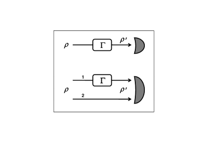
Figure 1: Single- and two-mode schemes for the detection of losses. Top: a single-mode squeezed thermal state $\rho$ enters the lossy channel with damping rate $\Gamma$. A measurement apparatus detects the output state $\rho^{\prime}$. Bottom: the lossy channel acts on the probing mode (1) of a two-mode squeezed thermal state $\rho$, while the reference mode (2) bypasses the channel. The output state $\rho^{\prime}$ of both the modes is then measured.

The propagation of a mode of radiation in a lossy channel corresponds to the coupling of the mode $a$ with a zero temperature reservoir made of large number of external modes. By assuming a Markovian reservoir and weak coupling between the system and the reservoir the dynamics of the system is described by the Lindblad Master equation Walls

$$\dot{\rho}=\frac{\Gamma}{2}\mathcal{L}[a]\rho$$ (22)

where $\mathcal{L}[a]\rho=2a\rho a^{\dagger}-a^{\dagger}a\rho-\rho a^{\dagger}a$. The general solution may be expressed by using the operator-sum representation of the associated completely-positive map, i.e., upon writing $\eta=e^{-\Gamma t}$, we have

$$\varrho(\eta)=\sum_{m}V_{m}\varrho V_{m}^{{\dagger}}$$

where

$$V_{m}=\sqrt{\frac{(1-\eta)^{m}}{m!}}a^{m}\eta^{\frac{1}{2}(a^{{\dagger}}a-m)}\,,$$

and $\varrho$ is the initial state.

V.1 Single-mode case

Let us now start with single-mode states. Eq. (22) can be recast into a Fokker-Planck equation for the Wigner function in terms of the quadrature variables $q$ and $p$,

$$\dot{W}=\frac{\Gamma}{2}\left[\partial_{\boldsymbol{X}}^{T}\boldsymbol{X}+\partial_{\boldsymbol{X}}^{T}\boldsymbol{\sigma}_{\infty}\partial_{\boldsymbol{X}}^{T}\right]W$$

where $\boldsymbol{X}=(q,p)^{T}$, $\partial_{\boldsymbol{X}}=(\partial_{q},\partial_{p})^{T}$ and we introduced the diffusion matrix $\boldsymbol{\sigma}_{\infty}=\text{diag}(1/2,1/2)$. Solving the equation for the Wigner function of a single-mode Gaussian state one can obtain the evolution equation for the CM $\boldsymbol{\sigma}$. This is given by AS1

$$\dot{\boldsymbol{\sigma}}=-\Gamma(\boldsymbol{\sigma}-\boldsymbol{\sigma}_{\infty})~{},$$

which yields to

$$\boldsymbol{\sigma}(t)=e^{-\Gamma t}\boldsymbol{\sigma}_{0}+(1-e^{-\Gamma t}){\boldsymbol{\sigma}}_{\infty}~{}.$$

The latter equation describes the evolution of an initial Gaussian state with CM $\boldsymbol{\sigma}_{0}$ towards the stationary state given by the Gaussian state of the environment with CM $\boldsymbol{\sigma}_{\infty}$. For simplicity, from now on we omit the index of $\boldsymbol{\sigma}_{0}$, we replace $\boldsymbol{\sigma}(t)\rightarrow\boldsymbol{\sigma}^{\prime}$, and we insert the time $t$ into the damping parameter $\Gamma$. Thus, the evolved CM of the single mode case simply reads

$$\boldsymbol{\sigma}^{\prime}=e^{-\Gamma}\boldsymbol{\sigma}+(1-e^{-\Gamma})\,\boldsymbol{\sigma}_{\infty}~{}.$$

Now let us consider the specific case of an input squeezed thermal state $\rho=\rho(r,n_{T})$ with squeezing $r$ and thermal number $n_{T}$. According to Eqs. (10) and (12), its CM is given by

$$\boldsymbol{\sigma}=\left(\begin{array}[c]{cc}a&0\\ 0&b\end{array}\right)~{},$$

with

$$a=\frac{1}{2}\left(1+2n_{\scriptstyle T}\right)e^{2r}~{},~{}b=\frac{1}{2}\left(1+2n_{\scriptstyle T}\right)e^{-2r}\,~{}.$$ (23)

At the output of the channel, the state $\rho^{\prime}$ has CM

$$\boldsymbol{\sigma}^{\prime}=\left(\begin{array}[c]{cc}a_{\Gamma}&0\\ 0&b_{\Gamma}\end{array}\right)~{},$$

where

$$a_{\Gamma}=\frac{1}{2}\left(1+2n_{\Gamma}\right)e^{2r_{\Gamma}}~{},~{}b_{\Gamma}=\frac{1}{2}\left(1+2n_{\Gamma}\right)e^{-2r_{\Gamma}}~{},$$ (24)

and

$$n_{\Gamma} =\sqrt{\det[\boldsymbol{\sigma}^{\prime}]}-1/2$$ (25)

$$r_{\Gamma} =\frac{1}{4}\log\left[\frac{e^{-\Gamma}a+(1-e^{-\Gamma})/2}{e^{-\Gamma}b+(1-e^{-\Gamma})/2}\right].$$ (26)

Thus, we still have a squeezed thermal state $\rho^{\prime}=\rho^{\prime}(r_{\Gamma},n_{\Gamma})$ with squeezing $r_{\Gamma}$ and thermal number $n_{\Gamma}$. Now, the discrimination between a lossless ($\Gamma=0$) and a lossy channel ($\Gamma>0$) corresponds to the discrimination between the input state $\rho=\rho(r,n_{T})$ and the output one $\rho^{\prime}=\rho^{\prime}(r_{\Gamma},n_{\Gamma})$. In order to estimate the error probability affecting this discrimination, we can compute the quantum Chernoff bound. This is achieved by replacing

$$(r,\bar{n})\rightarrow(r,n_{T})\;\;\hbox{and}\;\;(r^{\prime},\bar{n}^{\prime})\rightarrow(r_{\Gamma},n_{\Gamma})\,$$

in Eq. (20).

V.2 Two-mode case

According to the scheme of Fig. 1, the map describing the evolution of a two-mode state is $\mathcal{E}_{\Gamma}\otimes\mathcal{I}$, where the lossy channel $\mathcal{E}_{\Gamma}$ acts on the probing mode while the identity channel $\mathcal{I}$ acts on the reference mode. At the level of the CM it corresponds to the following transformation

$$\boldsymbol{\sigma}^{\prime}= \left(e^{-\Gamma/2}{\mathbb{I}}_{2}\oplus{\mathbb{I}}_{2}\right)\boldsymbol{\sigma}\left(e^{-\Gamma/2}{\mathbb{I}}_{2}\oplus{\mathbb{I}}_{2}\right)$$

$$+({\mathbb{I}}_{4}-e^{-\Gamma}{\mathbb{I}}_{2}\oplus{\mathbb{I}}_{2})\boldsymbol{\sigma}_{\infty}~{}.$$ (27)

As input state, let us consider a two-mode squeezed thermal state $\rho=\rho(r,n_{\scriptstyle T_{1}},n_{\scriptstyle T_{2}})$. Its CM is provided in Eq. (15) with the elements given in Eq. (16) by replacing $(r,\bar{n}_{1},\bar{n}_{2})\rightarrow(r,n_{\scriptstyle T_{1}},n_{\scriptstyle T_{2}})$. The CM of the output state can be derived using the Eq. (27). This CM can be put in the normal form of Eq. (15) with elements given by Eq. (16) by replacing $(r,\bar{n}_{1},\bar{n}_{2})\rightarrow(r_{\Gamma},n_{\scriptstyle\Gamma_{1}},n_{\scriptstyle\Gamma_{2}})$. Here the squeezing parameter $r_{\Gamma}$ and the thermal numbers $n_{\scriptstyle\Gamma_{1}}$ and $n_{\scriptstyle\Gamma_{2}}$ are function of the input parameters $r$, $n_{\scriptstyle T_{1}}$ and $n_{\scriptstyle T_{2}}$ (the explicit expression is too long to be shown here). Thus, the output state is still a two-mode squeezed thermal state $\rho^{\prime}=\rho^{\prime}(r_{\Gamma},n_{\scriptstyle\Gamma_{1}},n_{\scriptstyle\Gamma_{2}})$.

As before, the discrimination between a lossless ($\Gamma=0$) and a lossy channel ($\Gamma>0$) corresponds to the discrimination between the input state $\rho=\rho(r,n_{\scriptstyle T_{1}},n_{\scriptstyle T_{2}})$ and the output one $\rho^{\prime}=\rho^{\prime}(r_{\Gamma},n_{\scriptstyle\Gamma_{1}},n_{\scriptstyle\Gamma_{2}})$. The error probability affecting this discrimination is estimated by the QCB which is computed by replacing $(r,\bar{n}_{1},\bar{n}_{2})\rightarrow(r,n_{\scriptstyle T_{1}},n_{\scriptstyle T_{2}})$ and $(r^{\prime},\bar{n}_{1}^{\prime},\bar{n}_{2}^{\prime})\rightarrow(r_{\Gamma},n_{\scriptstyle\Gamma_{1}},n_{\scriptstyle\Gamma_{2}})$ in Eq. (21).

VI Optimization of the thermal probes

In this section, we optimize the discrimination of a lossless ($\Gamma=0$) from a lossy channel ($\Gamma>0$) by maximizing over thermal probes, i.e., single- and two-mode squeezed thermal states. For this sake, we evaluate the QCB as a function of the most important parameters of the input state, i.e., its total energy and squeezing. In our first analysis, we show that for fixed total energy, single- and two-mode squeezed vacuum states are optimal. In particular, we show the conditions where the two-mode state outperforms the single-mode counterpart. Then, by fixing both the total energy and squeezing, we will find the optimal squeezed thermal state. According to Sec. II the minimization of the QCB over single-copy states implies the minimization over multi-copy states (when the minimization is unconstrained or subject to single-copy constraints). This implies that finding the optimal input state $\rho$ at fixed energy automatically assures that $\rho\otimes\rho\otimes\cdots$ is the optimal multi-copy state at fixed energy per copy when we consider a multiple access to the unknown (memoryless) channel.

In order to perform our investigation we introduce a suitable parametrization of the input energy. Given a single-mode squeezed thermal state $\rho=\rho(r,n_{T})$, its energy (mean total number of photons) can be written as

$$N_{1}=n_{\scriptstyle T}+n_{\scriptstyle S}+2n_{\scriptstyle S}n_{\scriptstyle T}~{},$$ (28)

where $n_{\scriptstyle T}$ accounts for the mean number of thermal photons, $n_{\scriptstyle S}=\sinh^{2}r$ quantifies the squeezing, and $n_{\scriptstyle S}n_{\scriptstyle T}$ is a cross term. Alternatively, we can introduce a squeezing factor $\beta_{1}\in[0,1]$ such that

$$n_{\scriptstyle S} =\beta_{1}N_{1}$$ (29)

$$n_{\scriptstyle T} =\frac{(1-\beta_{1})N_{1}}{1+2\beta_{1}N_{1}}~{}.$$ (30)

Thus the single-mode squeezed thermal state can be parametrized as $\rho=\rho(N_{1},\beta_{1})$, i.e., in terms of its total energy $N_{1}$ and the squeezing factor $\beta_{1}$. Note that for $\beta_{1}=0$ the state is completely thermal with energy $N_{1}=n_{\scriptstyle T}$, while for $\beta_{1}=1$ the state is a squeezed vacuum with energy $N_{1}=n_{\scriptstyle S}$. In our problem of loss detection ($\Gamma=0$ versus $\Gamma>0$), we denote by $Q_{1}(N_{1},\beta_{1})$ the output QCB which is computed by using the input state $\rho=\rho(N_{1},\beta_{1})$.

Now, given a two-mode squeezed thermal state $\rho=\rho(r,n_{\scriptstyle T_{1}},n_{\scriptstyle T_{2}})$, its total energy can be written as

$$N_{2}=n_{\scriptstyle T_{1}}+n_{\scriptstyle T_{2}}+2n_{\scriptstyle S}+2n_{\scriptstyle S}(n_{\scriptstyle T_{1}}+n_{\scriptstyle T_{2}})~{},$$ (31)

where $n_{\scriptstyle T_{1}}$ ($n_{\scriptstyle T_{2}}$) quantifies the thermal photons in the probing (reference) mode, $n_{\scriptstyle S}=\sinh^{2}r$ quantifies the two-mode squeezing energy, and the last energetic term is a cross term. In this case, besides the squeezing factor $\beta_{2}$, we can also introduce an asymmetry parameter $\gamma\in[0,1]$ which quantifies the fraction of thermal energy used for the probing mode. In other words, we can write

$$n_{\scriptstyle S} =\frac{1}{2}\beta_{2}N_{2}$$ (32)

$$n_{\scriptstyle T_{1}} =\gamma\,\frac{(1-\beta_{2})N_{2}}{1+\beta_{2}N_{2}}$$ (33)

$$n_{\scriptstyle T_{2}} =(1-\gamma)\frac{(1-\beta_{2})N_{2}}{1+\beta_{2}N_{2}}.$$ (34)

Thus the two-mode squeezed thermal state can be parametrized as $\rho=\rho(N_{2},\beta_{2},\gamma)$, i.e., in terms of the total energy $N_{2}$, the squeezing factor $\beta_{2}$, and the asymmetry parameter $\gamma$. Note that for $\beta_{2}=0$ we have two thermal states, one describing the probing mode with thermal energy $n_{\scriptstyle T_{1}}=\gamma\,N_{2}$, and the other one describing the reference mode with thermal energy $n_{\scriptstyle T_{2}}=(1-\gamma)N_{2}$. For $\beta_{2}=1$ we have instead a two-mode squeezed vacuum state with total energy $N_{2}=2n_{\scriptstyle S}$. In this case, the thermal energy is zero and $\gamma$ can be therefore arbitrary. In our problem of loss detection ($\Gamma=0$ versus $\Gamma>0$), we denote by $Q_{2}(N_{2},\beta_{2},\gamma)$ the output QCB which is computed by using the input state $\rho=\rho(N_{2},\beta_{2},\gamma)$.

VI.1 Optimal input at fixed total energy

In our first investigation we fix the mean total number of photons of the input state. In other words we fix

$$N_{1}=N_{2}=N~{}.$$ (35)

Then we minimize the output QCB among single-mode and two-mode squeezed thermal states. As a first step we compute the optimal quantities

$$Q_{1}(N) :=\inf_{\beta_{1}}Q_{1}(N,\beta_{1})$$ (36)

$$Q_{2}(N) :=\inf_{\beta_{2},\gamma}Q_{2}(N,\beta_{2},\gamma)~{}.$$ (37)

Then, we compare $Q_{1}(N)$ with $Q_{2}(N)$.

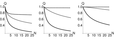
Figure 2: Output QCB$\ Q_{1}(N,\beta_{1})$ optimized over input single-mode squeezed thermal states $\rho=\rho(N,\beta_{1})$. From left to right we consider different values of the transmissivity: $\eta=0.1$ (left panel), $\eta=0.5$ (middle panel) and $\eta=0.9$ (right panel). In each panel, we plot $Q_{1}(N,\beta_{1})$ as function of the energy $N$ for different values of $\beta_{1}$. From top to bottom: $\beta_{1}=0.1$ (dashed line), $\beta_{1}=0.5$ (dotted line) and $\beta_{1}=1$ (solid line). The minimum curve is always achieved for $\beta_{1}=1$, i.e., for an input single-mode squeezed vacuum state.

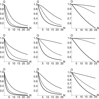
Figure 3: Output QCB$\ Q_{2}(N,\beta_{2},\gamma)$ optimized over input two-mode squeezed thermal states $\rho=\rho(N,\beta_{2},\gamma)$. From left to right we consider different values of the transmissivity: $\eta=0.1,$ $0.5$ and $0.9$. From top to bottom, we consider different values of the asymmetry parameter $\gamma=0,$ $0.5$ and $1$. In each panel, we then plot $Q_{2}$ as function of the energy $N$ for different values of $\beta_{2}$. From top to bottom: $\beta_{2}=0.1$ (dashed line), $\beta_{2}=0.5$ (dotted line) and $\beta_{2}=1$ (solid line). The minimum curve is always achieved for $\beta_{2}=1$ corresponding to an input two-mode squeezed vacuum state.

According to our findings, in the Eqs. (36) and (37) the infima are achieved for $\beta_{1}=\beta_{2}=1$. This is numerically shown in Fig. 2 for the single-mode case and in Fig. 3 for the two-mode case. Thus, we have found that, at fixed input energy $N$, the optimal thermal probes are given by single- and two-mode squeezed vacuum states. In this case, the input state is pure and the QCB corresponds to the fidelity (which is the case when the s-overlap in Eq. (3) is minimized for $s$ approching the border). Let us adopt the transmissivity $\eta=e^{-\Gamma}$ to quantify the damping of the channel, so that $\Gamma=0$ (ideal channel) corresponds to $\eta=1$, and $\Gamma>0$ (lossy channel) corresponds to $0\leq\eta<1$. Then, for single-mode we can write

$$Q_{1}(N)=\frac{1}{\sqrt{1+N(1-\eta^{2})}}~{},$$ (38)

and for two-modes we derive

$$Q_{2}(N)=\frac{4}{\left[2+N(1-\sqrt{\eta})\right]^{2}}~{}.$$ (39)

In Fig. 4, we show the behaviors of the single-mode QCB $Q_{1}(N)$ and two-mode QCB $Q_{2}(N)$ as function of the input energy $N$ for several values of transmissivity $\eta$ (or, equivalently, the damping rate $\Gamma$). As expected the discrimination improves by increasing the input energy $N$ and decreasing the transmissivity $\eta$.

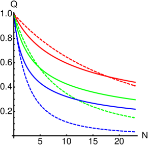
Figure 4: (Color online). Single-mode QCB $Q_{1}(N)$ (solid lines) and two-mode QCB $Q_{2}(N)$ (dashed lines) as a function of the input energy $N$ for different damping rates. From top to bottom $\Gamma=0.1,0.3,1$ (red, green and blue, respectively) corresponding to $\eta\simeq 0.9,0.74,0.37$. By comparing curves with the same color (fixed damping $\Gamma$), we can see that $Q_{2}(N)$ outperforms $Q_{1}(N)$ only after a certain value of the input energy $N$.

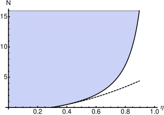
Figure 5: Threshold energy as a function of the transmissivity $N_{th}=N_{th}(\eta)$ (solid curve dividing the dark and the white areas). The dark area indicates the values of the energy $N$ for which the two-mode squeezed vacuum state is optimal. The white region indicates where the single-mode squeezed vacuum state is optimal. The dashed line denotes the behavior of the threshold energy $N_{th}$ close to the critical transmissivity $\eta_{c}\simeq 0.296$.

As we can see from Fig. 4, for a given value of the transmissivity $\eta$, the two-mode QCB $Q_{2}(N)$ outperforms the single-mode QCB $Q_{1}(N)$ only after a threshold energy. In fact, for any value of the transmissivity $\eta$ larger than a critical value $\eta_{c}$ there is a threshold energy $N_{th}=N_{th}(\eta)$ that makes the two-mode squeezed vacuum state more convenient than the single-mode counterpart. This threshold energy decreases for decreasing values of $\eta$. In particular, for transmissivities less than the critical value $\eta_{c}$, the threshold energy becomes zero, i.e., the two-mode state is always better than single-mode state. We have numerically evaluated the critical value $\eta_{c}\simeq 0.296$ (corresponding to $\Gamma_{c}\simeq 1.22$). This phenomenon is fully illustrated in Fig. 5, where we have plotted the threshold energy as function of the transmissivity $N_{th}=N_{th}(\eta)$. For $N>N_{th}$ (dark area), the optimal state is the two-mode squeezed vacuum state, while for $N<N_{th}$ (white area) it is the single-mode squeezed vacuum state. In particular, note that $N_{th}=0$ at $\eta=\eta_{c}$. Close to the critical transmissivity we have OtherCurve

$$N_{th}\simeq 4(\eta-\eta_{c})+5.5(\eta-\eta_{c})^{2}~{}.$$ (40)

VI.2 Optimal input at fixed energy and squeezing

It should be said that, in realistic conditions, it is unlikely to have pure squeezing. For this reason, it is important to investigate the performances of the squeezed thermal states by fixing this physical parameter together with the total energy. Thus, in this section, we fix both the input energy and squeezing, i.e., we set

$$N_{1} =N_{2}=N,$$

$$\beta_{1} =\beta_{2}=\beta~{}~{}(0\leq\beta\leq 1)~{}.$$ (41)

Then, we compare the single-mode squeezed thermal state $\rho=\rho(N,\beta)$ with the two-mode squeezed thermal states $\rho=\rho(N,\beta,\gamma)$ for various values of $\gamma$. In other words, we compare $Q_{1}(N,\beta)$ and $Q_{2}(N,\beta,\gamma)$.

For fixed $N$ and $\beta$, we find that the minimum of $Q_{2}(N,\beta,\gamma)$ is achieved for $\gamma=1$ (easy to check numerically). This means that two-mode discrimination is easier when all the thermal photons are sent through the lossy channel. In this case we find numerically that

$$Q_{2}(N,\beta,1)<Q_{1}(N,\beta)\,,$$

for every values of the input parameters $N$ and $\beta$, and every value of damping rate $\Gamma$ in the channel. In other words, at fixed energy and squeezing, there is a two-mode squeezed thermal state (the asymmetric one with $\gamma=1$) able to outperform the single-mode squeezed thermal state in the detection of any loss. In order to quantify the improvement we introduce the QCB reduction

$$\Delta Q=Q_{1}(N,\beta)-Q_{2}(N,\beta,1).$$

The more positive this quantity is, the more convenient is the use of the two-mode state instead of the single-mode one. In Fig. 6 we show the behavior of $\Delta Q$ as function of the input energy and squeezing for two different values of the damping. As one can see from the plot, the QCB reduction is always positive. Its value increases with the energy while reaching a maximum for intermediate values of the squeezing. By comparing the two panels of Fig. 6, we can also note that the QCB reduction increases for increasing damping $\Gamma$ (i.e., decreasing transmissivity).

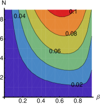
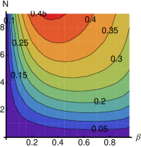
Figure 6: (Color online) Density plot of the QCB reduction $\Delta Q$ as function of the input energy $N$ and the squeezing $\beta$. The left plot is for $\Gamma=0.1$ and the right one for $\Gamma=0.9$.

Thus, we have just shown that, for fixed values of $N$ and $\beta$, the asymmetric two-mode squeezed thermal state ($\gamma=1$) is the optimal thermal probe in the detection of any loss $\Gamma$. Here we also show that this is approximately true for $\gamma\lesssim 1$. In other words, we show that the inequality $Q_{2}(N,\beta,\gamma)<Q_{1}(N,\beta)$ is robust against fluctuations of $\gamma$ below the optimal value $\gamma=1$. This property is clearly important for practical implementations. To study this situation, let us consider the $\gamma$-dependent QCB reduction

$$\Delta Q_{\gamma}=Q_{1}(N,\beta)-Q_{2}(N,\beta,\gamma)~{}.$$ (42)

In Fig. 7 we have specified this quantity for different values of the asymmetry parameter $\gamma$ (each panel refers to a different value of $\gamma$). Then, for every chosen $\gamma$, we have computed $\Delta Q_{\gamma}$ over a sample of $10^{3}$ random values of $N$, $\beta$, and $\Gamma$ (in each panel). As one can see from the figure, the quantity $\Delta Q_{\gamma}$ is approximately positive also when $\gamma$ is quite different from the unity.

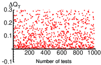
Figure 7: (Color online) QCB reduction $\Delta Q_{\gamma}$ for different values of $\gamma$ (top left $\gamma=0.99$, top right $\gamma=0.9$, bottom left $\gamma=0.8$, bottom right $\gamma=0.7$). In each panel, $\Delta Q_{\gamma}$ is computed over a sample of $10^{3}$ random values of $N$, $\beta$, and $\Gamma$.

VII Analysis of the correlations

Since two-mode squeezed thermal states are able to outperform the single-mode counterpart under several physical conditions, it is natural to investigate this improvement directly in terms of the correlations of the input state. The quantification of the correlations is realized by using the entanglement, the quantum discord and the quantum mutual information. In order to quantify the degree of entanglement of a two-mode Gaussian state, we can use the logarithmic negativity. Let us consider a bipartite Gaussian state with CM given in Eq. (13). It is easy to derive the symplectic eigenvalues of the partially transposed state. These are given by

$$\tilde{d}_{\pm}=\sqrt{\frac{\tilde{\Delta}-\sqrt{\tilde{\Delta}^{2}-4I_{4}}}{2}}~{},$$

where $\tilde{\Delta}=I_{1}+I_{2}-2I_{3}$, and the symplectic invariants $I_{1}$, $I_{2}$, $I_{3}$ and $I_{4}$ are defined in Eq. (14). From the smallest of these symplectic eigenvalues, we can compute the logarithmic negativity, which is equal to

$$E=\max\{0,-\log 2\tilde{d}_{-}\}~{}.$$

A bipartite Gaussian state is entangled iff $\tilde{d}_{-}<1/2$, so that the logarithmic negativity gives positive values for all the entangled states and $0$ otherwise.

The quantum discord is defined as the mismatch of two different quantum analogues of classically equivalent expressions of the mutual information and may be used to quantify quantum correlations in mixed separable states. For a two-mode squeezed thermal state with CM as in Eq. (15), the quantum discord may be written as GQDSCa

$$D= h(\sqrt{I_{2}})-h(d_{-})-h(d_{+})$$

$$+h\left(\frac{\sqrt{I_{1}}+2\sqrt{I_{1}I_{2}}+2I_{3}}{1+2\sqrt{I_{2}}}\right)$$ (43)

where

$$h(x)=\left(x+\frac{1}{2}\right)\log\left(x+\frac{1}{2}\right)-\left(x-\frac{1}{2}\right)\log\left(x-\frac{1}{2}\right)$$

is the binary Shannon entropy. We have that, for $0\leq D\leq 1$, the state may be either entangled or separable, whereas all the states with $D>1$ are entangled GQDSCa ; GQDSCb .

Finally, the quantum mutual information, which quantifies the amount of total, classical plus quantum, correlations, is given by $I=S(\rho_{A})+S(\rho_{B})-S(\rho_{AB})$, where $S(\rho)=-\mathop{\text{Tr}}\nolimits[\rho\log\rho]$ is the von Neumann entropy of the state $\rho$ and $\rho_{A(B)}=\mathop{\text{Tr}}\nolimits_{B(A)}[\rho_{AB}]$ are the partial traces over the two subsystems. For a two-mode squeezed thermal state with CM as in Eq. (15) the quantum mutual information can be computed using the formula

$$I=\frac{1}{2}\left[h(\sqrt{I_{1}})+h(\sqrt{I_{2}})-h(d_{+})-h(d_{-})\right]\,.$$

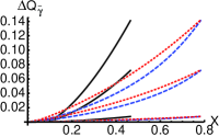
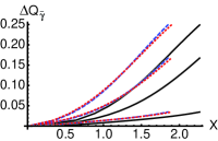
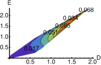
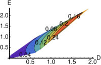
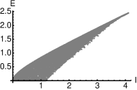
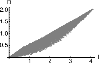
Figure 8: (Color online) Upper panels. QCB reduction $\Delta Q_{\bar{\gamma}}$ (with $\bar{\gamma}=0.999$) as a function of the three correlation quantifiers X=I,D,E where I is the quantum mutual information (dotted red), D is the quantum discord (dashed blue) and E is the entanglement (solid black). The plots are for fixed squeezing: $\beta=0.1$ for the left panel and $\beta=0.9$ for the right one. For each quantifier we plot three different curves corresponding to different values of the damping (from top to bottom $\Gamma=0.9,0.5$ and $0.1$). Each curve is generated by varying the input energy $N$ between $0$ and $5$ photons. Middle panels. Density plots of the QCB reduction $\Delta Q_{\bar{\gamma}}$ as a function of the input discord and entanglement. The plots are for fixed damping: $\Gamma=0.2$ in the left panel and $\Gamma=0.8$ in the right one. In each panel, the density plot is generated by varying the squeezing $0\leq\beta\leq 1$ and the energy $0\leq N\leq 5$. Lower panels. Entanglement (left) and discord (right) as a function of the quantum mutual information. Plots are generated by taking a random sample of $10^{4}$ two-mode squeezed thermal states, i.e., random values of $N$ and $\beta$ with $\gamma=\bar{\gamma}$.

For pure states the previous three measures are equivalent, whereas for mixed states, as in the case under investigation in this section, they generally quantify different kind of correlations. Here we consider the QCB reduction $\Delta Q_{\bar{\gamma}}=Q_{1}(N,\beta)-Q_{2}(N,\beta,\bar{\gamma})$ between a single-mode squeezed thermal state $\rho=\rho(N,\beta)$ and a two-mode squeezed thermal state $\rho=\rho(N,\beta,\bar{\gamma})$ with $\bar{\gamma}=0.999$. By fixing the input squeezing $\beta$ and varying the input energy $N$, we study the behaviour of $\Delta Q_{\bar{\gamma}}$ as function of the three correlation quantifiers, i.e., quantum mutual information, quantum discord and entanglement (computed over the input two-mode state).

As shown in the upper panels of Fig. 8, the QCB reduction $\Delta Q_{\bar{\gamma}}$ is an increasing function of all the three correlation quantifiers for fixed input squeezing ($\beta=0.1$ for the left panel and $\beta=0.9$ for the right one). Note that, in each panel and for each quantifier, we plot three different curves corresponding to different values of the damping $\Gamma=0.9,$ $0.5$ and $0.1$. The monotonicity of the QCB reduction in all the correlation quantifiers suggests that the presence of correlations should definitely be considered as a resource for loss detection, whether these correlations are classical or genuinely quantum, i.e., those quantified by entanglement. In other words, employing the input squeezing in the form of correlations is always beneficial for loss detection when we consider squeezed thermal states as input sources. The importance of correlations is confirmed by the plots in the middle panels. Here we consider again the QCB reduction $\Delta Q_{\bar{\gamma}}=Q_{1}(N,\beta)-Q_{2}(N,\beta,\bar{\gamma})$ for $\bar{\gamma}=0.999$. Then, by varying input squeezing $\beta$ and energy $N$, we study $\Delta Q_{\bar{\gamma}}$ as function of both discord and entanglement (damping is $\Gamma=0.2$ in the left panel, and $\Gamma=0.8$ in the right one). These plots show how the QCB reduction is approximately an increasing function of both discord and entanglement. Finally, in the lower panels of Fig. 8, we also show how entanglement (left) and discord (right) are increasing functions of the quantum mutual information with good approximation (these plots are generated by choosing a random sample of $10^{4}$ two-mode squeezed thermal states).

VIII Conclusions

In this paper we have considered the quantum discrimination of lossy channels. In particular, we have focused to the case when one of the two channels is the identity, i.e., the problem of discriminating the presence of a damping process from its absence (loss detection). For this kind of discriminination we have considered thermal probes as input, i.e., single- and two-mode squeezed thermal states. The performance of the channel discrimination has been quantified using the QCB, computed over the two possible states at the output of the unknown channel for a given input state. Finding the optimal input state $\rho$ which minimizes this bound gives automatically the optimal multi-copy state $\rho\otimes\rho\otimes\cdots$ when we consider many accesses to the unknown channel (under the assumption of single-copy constraints). In this scenario, we have fixed the total energy of the input state and optimized the discrimination (detection of loss) over the class of single- and two-mode squeezed thermal states. We have found numerically that the optimal states are pure, thus corresponding to single- and two-mode squeezed vacuum states. Furthermore, we have determined the conditions where the two-mode state outperforms the single-mode counterpart. This happens when the energy exceeds a certain threshold, which becomes zero for suitably low values of the transmissivity (i.e., high values of damping).

It is worth noticing that our approach (where we fix the total energy of probing and reference modes) also gives a sufficient condition for the problem where only the probing energy is fixed. In fact, if a two-mode state outperforms a single-mode state above a certain threshold value $N_{th}$ of the total energy, this also happens when just the energy of the probing mode is above that value $N_{th}$. This is a trivial consequence of the fact that the total energy is bigger than the probing energy for two-mode states ($N_{2}>N_{2}^{\mathrm{probe}}$) while the two quantities are the same for single-mode states ($N_{1}=N_{1}^{\mathrm{probe}}$). Thus, $N_{2}^{\mathrm{probe}}=N_{1}^{\mathrm{probe}}>N_{th}$ can be written as $N_{2}>N_{1}>N_{th}$ which is a stronger condition than $N_{2}=N_{1}>N_{th}$, since the QCB is decreasing in the total energy, as one can see from Eqs. (38) and (39).

In our investigation we have then considered the problem of loss detection in more realistic conditions, where it is unlikely to have pure squeezing. In this case, we have studied the optimal state for fixed total energy and squeezing, i.e., by fixing all the relevant resources needed to create the input state. Under these constraints, we have shown that a two-mode squeezed thermal state which conveys all the thermal photons in the dissipative channel is the optimal thermal probe. In addition, this result is robust against fluctuations, i.e., it holds approximately also when the thermal photons are distributed in a more balanced way between the probe mode (sent through the dissipative channel) and the reference mode (bypassing the channel).

Finally we have closely investigated the role of correlations in our problem of loss detection. We have found that, for fixed input squeezing, the reduction of the QCB is an increasing function of several correlation quantifiers, such as the quantum entanglement, the quantum discord and the quantum mutual information. We then verify that employing the input squeezing in the form of correlations (quantum or classical) is always beneficial for the detection of loss by means of thermal probes.

The results of our paper provides new elements in the field of quantum channel discrimination and can be applied to a wide range applications, including the characterization of absorbing materials. In particular, they are relevant in all the situations where the physical constraints regard the creation of the input resources rather than the channel to be discriminated.

References

- (1) H.-P. Breuer and F. Petruccione, The Theory of Open Quantum Systems (Oxford University Press, Oxford, 2002).
- (2) A. Serafini, M. G. A. Paris, F. Illuminati, and S. De Siena, J. Opt. B 7, R19 (2006).
- (3) V. D’Auria, C. de Lisio, A. Porzio, S. Solimeno, and M. G. A. Paris, J. Phys. B 39, 1187 (2006).
- (4) W. H. Zurek, Rev. Mod. Phys. 75, 715 (2003).
- (5) J. B. Brask, I. Rigas, E. S. Polzik, U. L. Andersen, and A. S. Sørensen, Phys. Rev. Lett. 105, 160501 (2010).
- (6) K. Jensen, W. Wasilewski, H. Krauter, T. Fernholz, B. M. Nielsen, M. Owari, M. B. Plenio, A. Serafini, M. M. Wolf and E. S. Polzik, Nature Phys. 7, 13 (2011).
- (7) M. Brune, J. Bernu, C. Guerlin, S. Deléglise, C. Sayrin, S. Gleyzes, S. Kuhr, I. Dotsenko, J. M. Raimond, and S. Haroche, Phys. Rev. Lett. 101, 240402 (2008); S. Deléglise, I. Dotsenko, C. Sayrin, J. Bernu, M. Brune, J. Raymond, and S. Haroche, Nature 455, 510 (2008).
- (8) H. Wang, M. Hofheinz, M. Ansmann, R.C. Bialczak, E. Lucero, M. Neeley, A. D. O’Connell, D. Sank, J. Wenner, A. N. Cleland, and John M. Martinis, Phys. Rev. Lett. 101, 240401 (2008).
- (9) S. L. Braunstein, and H. J. Kimble, Phys. Rev. Lett. 80, 869 (1998); P. van Loock, and S. L. Braunstein, Phys. Rev. Lett. 84, 3482 (2000); S. Pirandola, S. Mancini, D. Vitali, and P. Tombesi, Phys. Rev. A 68, 062317 (2003); S. Pirandola, S. Mancini, D. Vitali, and P. Tombesi, J. Mod. Opt. 51, 901 (2004); S. Pirandola and S. Mancini, Laser Physics 16, 1418 (2006).
- (10) C. Weedbrook, A. M. Lance, W. P. Bowen, T. Symul, T. C. Ralph, and P. K. Lam, Phys. Rev. Lett. 93, 170504 (2004); C. Weedbrook, S. Pirandola, S. Lloyd, T. C. Ralph, Phys. Rev. Lett. 105, 110501 (2010).
- (11) S. Pirandola, S. L. Braunstein, and S. Lloyd, Phys. Rev. Lett. 101, 200504 (2008); S. Pirandola, S. Mancini, S. Lloyd, and S. L. Braunstein, Nature Physics 4, 726 (2008).
- (12) I. Devetak and A. Winter, Phys. Rev. Lett. 93, 080501 (2004).
- (13) S. Pirandola, R. García-Patrón, S. L. Braunstein, and S. Lloyd, Phys. Rev. Lett. 102, 050503 (2009); R. García-Patrón, S. Pirandola, S. Lloyd, and J. H. Shapiro, Phys. Rev. Lett. 102, 210501 (2009).
- (14) A. Monras and F. Illuminati, Phys. Rev. A 83, 012315 (2011).
- (15) S. Pirandola, Phys. Rev. Lett. 106, 090504 (2011).
- (16) R. Nair, “Discriminating quantum optical beam-splitter channels with number diagonal signal states: applications to quantum reading and target detection”, arXiv:1105.4063.
- (17) S.-H. Tan, B. I. Erkmen, V. Giovannetti, S. Guha, S. Lloyd, L. Maccone, S. Pirandola, and J. H. Shapiro, Phys. Rev. Lett. 101, 253601 (2008).
- (18) S. Lloyd, Science 321, 1463 (2008); J. H. Shapiro and S. Lloyd, New J. Phys. 11, 063045 (2009); H. P. Yuen and R. Nair, Phys. Rev A 80, 023816 (2009); S. Guha and B. Erkmen, ibid. 80, 052310 (2009); A. R. Usha Devi and A. K. Rajagopal, ibid. 79, 062320 (2009).
- (19) V. D’Auria, S. Fornaro, A. Porzio, S. Solimeno, S. Olivares, and M. G. A. Paris, Phys. Rev. Lett. 102, 020502 (2009).
- (20) E. C. G. Sudarshan, Phys. Rev. Lett. 10, 277 (1963); R. J. Glauber, Phys. Rev. 131, 2766 (1963).
- (21) H. Venzl and M. Freyberger, Phys. Rev. A 75, 042322 (2007).
- (22) A. Monras, M. G. A. Paris, Phys. Rev. Lett. 98, 160401 (2007).
- (23) G. Adesso, F. Dell’Anno, S. De Siena, F. Illuminati, and L. A. M. Souza, Phys. Rev. A 79, 040305(R) (2009).
- (24) A. Monras and F. Illuminati, Phys. Rev. A 81, 062326 (2010).
- (25) C. W. Helstrom, Quantum Detection and Estimation Theory (Academic Press, New York, 1976).
- (26) A. Chefles, Contemp. Phys. 41, 401 (2000).
- (27) J. A. Bergou, U. Herzog, M. Hillery in Quantum State Estimation, Lect. Not. Phys. 649, J. Rehacek, M. G. A. Paris (Eds) (Springer, Berlin, 2004), pp 417-465.
- (28) A. Chefles in Quantum State Estimation, Lect. Not. Phys. 649, J. Rehacek, M. G. A. Paris (Eds) (Springer, Berlin, 2004), pp 467-511.
- (29) V. Kargin, Ann. Stat. 33, 959 (2005).
- (30) J. Calsamiglia, R. Munoz-Tapia, L. Masanes, A. Acín, E. Bagan, Phys. Rev. A 77, 032311 (2008).
- (31) K. M. R. Audenaert, J. Calsamiglia, R. Munoz-Tapia, E. Bagan, Ll. Masanes, A. Acin, F. Verstraete, Phys. Rev. Lett. 98, 160501 (2007).
- (32) M. Nussbaum, and A. Szkola, Ann. Stat. 37, 1040 (2009).
- (33) K. M. R. Audenaert, M. Nussbaum, A. Szkola, and F. Verstraete, Commun. Math. Phys. 279, 251 (2008).
- (34) S. Pirandola and S. Lloyd, Phys. Rev. A 78, 012331 (2008).
- (35) H. Ollivier, W. H. Zurek, Phys. Rev. Lett. 88, 017901 (2001); W. H. Zurek, Phys. Rev. A 67, 012320 (2003).
- (36) C. A. Rodriguez-Rosario, K. Modi, A. Kuah, A. Shaji, and E. C. G. Sudarshan, J. Phys. A 41, 205301 (2008); M. Piani, P. Horodecki, and R. Horodecki, Phis. Rev. Lett. 100, 090502 (2008).
- (37) A. Ferraro, L. Aolita, D. Cavalcanti, F. M. Cucchietti, and A. Acin, Phys. Rev. A 81, 052318 (2010).
- (38) P. Giorda and M. G. A. Paris, Phys. Rev. Lett. 105, 020503 (2010).
- (39) G. Adesso and A. Datta, Phys. Rev. Lett. 105, 030501 (2010).
- (40) V. Vedral, Rev. Mod. Phys. 74, 197 (2002).
- (41) M. Boca, I. Ghiu, P. Marian, and T. A. Marian, Phys. Rev. A 79, 014302 (2009).
- (42) I. Ghiu, G. Björk, P. Marian, and T. A. Marian, Phys. Rev. A 82, 023803 (2010).
- (43) D. F. Abasto, N. T. Jacobson, P. Zanardi, Phys. Rev. A 77, 022327 (2008).
- (44) C. Invernizzi, M. G. A. Paris, J. Mod. Opt 57, 1362 (2010).
- (45) A. Ferraro, S. Olivares, M. G. A. Paris, Gaussian States in Quantum Information (Bibliopolis, Napoli 2005).
- (46) S. L. Braunstein and A. K. Pati, Quantum Information Theory with Continuous Variables (Kluwer Academic, Dordrecht, 2003).
- (47) C.A. Fuchs and J. V. de Graafs, IEEE Trans. Inf. Theory 45, 1216 (1999).
- (48) M. A. Nielsen and I. L. Chuang, Quantum Computation and Quantum Information (Cambridge University Press, Cambridge, 2000).
- (49) S. Pirandola, Phys. Rev. Lett. 106, 090504 (2011): Online Supplementary Material (http://link.aps.org/ supplemental/10.1103/PhysRevLett.106.090504).
- (50) Note that, in our derivations, what is important is the modulus of the squeezing parameter but not its sign. As a result, we can choose as well as .
- (51) A. Serafini, F. Illuminati, and S. de Siena, J. Phys. B 37, L21 (2004).
- (52) S. Pirandola, A. Serafini, and S. Lloyd, Phys. Rev. A 79, 052327 (2009).
- (53) Note that, because of the continuity of the QCB, the error probability in the discrimination between a lossy channel () and an almost-ideal channel () can be made arbitrarily close to the error probability affecting the discrimination of the same lossy channel () and an ideal channel ().
- (54) D. F. Walls and G. J. Milburn, Quantum Optics (Springer, Berlin, 1994).
- (55) A. Serafini, F. Illuminati, M. G. A. Paris, S. De Siena, Phys. Rev A 69, 022318 (2004).
- (56) Clearly we can invert the curve and introduce a threshold transmissivity as function of the energy . For values the two-mode state is better than the single-mode state, while the opposite happens for . We have for small and for large .