THE QUANTUM ORIGIN OF COSMIC STRUCTURE

In this concise, albeit subjective review of structure formation, I shall introduce the cosmological standard model and its theoretical and observational underpinnings. I will focus on recent results and current issues in theoretical cosmology, in particular in cosmological perturbation theory and its applications.

1 Introduction

Recent years have seen a remarkable transformation of cosmology, from a rather esoteric subject at the borderline of theoretical physics and applied mathematics to one of the most vibrant and popular areas of modern Astronomy. This development has been brought about by the spectacular advance in the subject, such as the development of cosmological perturbation theory, but more importantly, by the availability of new observational data sets of unprecedented quantity and quality.

Two data sets are of particular importance in this context, Cosmic Microwave Background (CMB) experiments Large Scale Structure (LSS) surveys. The CMB experiments$\!{}^{{\bf?}}$ , balloon-borne, using dedicated satellites, or ground-based, have revolutionised our understanding of the universe, giving us access to information from the very early universe in form of tiny temperature anisotropies, at the level of $1$ part in $100,000$, imprinted on the CMB. The exceptionally successful Wmap satellite mission$\!{}^{{\bf?}}$ which started in June 2001 and ended just recently (see contribution by Hinshaw in this volume), measured the spectrum of these anisotropies with unprecedented precision on large and medium angular scales. The Planck mission$\!{}^{{\bf?}}$, launched in May 2009, is now taking data, and will not only improve temperature anisotropy measurements and extend them to smaller scales, but will also measure the polarisation of the CMB (see contribution by de Benardis in this volume). LSS surveys improved our understanding of the late universe. From measuring the positions and redshift distances from just hundreds or thousands of galaxies, the latest surveys, such as 2df Galaxy Redshift Survey$\!{}^{{\bf?}}$ (now completed), the 6df Galaxy Survey$\!{}^{{\bf?}}$ and the SDSS$\!{}^{{\bf?}}$ (both still taking data), have mapped hundreds of thousands of galaxies, and other objects, and eventually will have mapped on the order of millions of galaxies.

In the following sections I shall give a brief overview of our current understanding of structure formation, in particular how vacuum fluctuations in the fields present in the very universe give rise to CMB anisotropies and LSS in the late universe. I do apologise in advance for a rather incomplete and subjective referencing due to the limited space available.

2 The evolution of the Universe

Let us now turn to the evolution of the universe, that the observational data from CMB experiments and LSS surveys mentioned in the previous section and our understanding of fundamental physics suggest. In the following I shall describe the Cosmological standard model reflecting the general consensus in the cosmology community under the tacit understanding that nothing “too weird” is included.

Faced with the observational data, we might first ask what underlying theory or theories govern the evolution of the Universe, giving rise to the data. Fortunately we do not have to invoke utterly new physics to answer this question. Most of the progress in recent years is built on two familiar theories from theoretical physics, each governing their particular range of scales, namely on small scales Quantum Field Theory, necessary to set initial conditions for the universe, and on large scales Einstein’s General Relativity, necessary to calculate its evolution. This means we can already work with two separate, well understood theories, instead of having to wait for a more fundamental final theory. Although it would be nice to have an underlying more fundamental theory, we already have the tools to calculate how quantum fluctuations evolve into large scale structure, thereby testing models of the early universe which at least reflect some aspects of any more fundamental theory.

Figure 1 summarises the evolution of the universe in the cosmological standard model (figure from Faucher-Giguère et al.$\!{}^{{\bf?}}$).

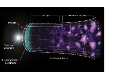
Figure 1: The evolution of the universe in what has become the cosmological standard model.

The universe begins with a period accelerated expansion, called inflation. During this era small quantum fluctuations in the fields present are stretched by the expansion of spacetime to super-horizon scales (larger than the particle horizon), where they are frozen in. These small fluctuations therefore remain constant until they later reenter the horizon and act as the “seeds” for the anisotropies in the CMB and source the formation of the LSS, where the small fluctuation are amplified through gravitational instability. Roughly $400,000$ years after the beginning of the universe the CMB is formed, followed by an epoch known as the “dark ages” during which no objects emitting visible light are present. The first stars are forming ca. 400 Myears afterwards, starting an epoch of reionisation ending roughly 1 Gyear after the beginning. The first galaxies begin to assemble during the dark ages, ever larger structures such as clusters and super-cluster of galaxies form thereafter, and the universe has begun to undergo another period of accelerated expansion a couple of Gyears ago. The main constituents of the universe as given by the seven year WMAP data (see Komatsu et al.$\!{}^{{\bf?}}$) at the present day are roughly 73% dark energy, 23% dark matter, and 4.5% baryonic matter.

Let me stress again, unlike the standard model in particle physics, the cosmological standard model is by no means accepted by the whole community working in the wider field of cosmology. This reflects on the one hand the heterogeneity of the field and the community, and on the other the still weaker experimental and observational “underpinnings” of cosmology compared to particle physics, despite the huge progress in recent years. The cosmological standard model is however the model most practitioners might agree upon, albeit some with a slight hesitation.

To understand the final “details” – what drives inflation, what drives the late time acceleration of the universe – we might need to resort to more arcane areas of theoretical physics. I will return to these questions later on.

3 Generating primordial density perturbations

In this section I shall briefly review how the primordial density perturbations that source the formation of the CMB anisotropies and the LSS are generated. As pointed out above, the dynamics of the universe on large and intermediate scales is controlled by Einstein equations

$$G_{\mu\nu}=8\pi\ G\ T_{\mu\nu}\,,$$ (1)

where $G_{\mu\nu}$ is the Einstein tensor describing the geometry of spacetime, $T_{\mu\nu}$ is the energy-momentum tensor encoding the matter content of the universe, and $G$ is Newton’s constant. However, the initial conditions are set by the theory governing the smallest scales, Quantum field theory. Of particular importance here will be the dynamics of the field driving inflation, the inflaton.

3.1 Inflation

Cosmological inflation was proposed in the early eighties by Starobinsky$\!{}^{{\bf?}}$ and Guth$\!{}^{{\bf?}}$ to alleviate several problems of the Hot Big Bang model (such as the flatness, horizon, monopole problems, see e.g. Liddle and Lyth$\!{}^{{\bf?}}$ for an introduction to modern cosmology). Inflation is a period of accelerated expansion of spacetime in the very early universe. This is “easily” achieved by introducing a scalar field ${\varphi}$ with potential $U$, which gives rise to the pressure $P=\frac{1}{2a^{2}}{\varphi}^{\prime 2}-U({\varphi})\,,$ where $a$ is the scale factor and a prime denotes differentiation with respect to conformal time $\eta$.

We can see that the pressure $P$ is negative during a period of potential domination, which is usually associated with the field “slowly rolling” down its potential, therefore having small or negligible kinetic energy (this is known as the slow-roll approximation).

The dynamics of the background is governed by the Klein-Gordon equation

$${\varphi}^{\prime\prime}+2{\cal H}{\varphi}^{\prime}+a^{2}U_{,{\varphi}}=0\,,$$ (2)

for the scalar field, and by the Friedmann equation

$${\cal H}^{2}=\frac{8\pi G}{3}\left(\frac{1}{2}{{\varphi}^{\prime}}^{2}+a^{2}U\right)\,,$$ (3)

for the scalar factor $a$, where ${\cal H}=a^{\prime}/a$. The above system constitutes a simple damped oscillator. Imposing the slow-roll approximation then gives a nearly constant Hubble parameter $H={\cal H}/a$.

We now turn to the generation of vacuum fluctuations in the scalar field. The evolution of these fluctuations is governed by the perturbed Klein-Gordon equation

$${\delta{\varphi}_{1}}^{\prime\prime}+2{\cal H}{\delta{\varphi}_{1}}^{\prime}+k^{2}{\delta{\varphi}_{1}}+a^{2}U_{,{\varphi}{\varphi}}{\delta{\varphi}_{1}}=0$$ (4)

where we assumed slow-roll and are working in Fourier space, with $k$ being the comoving wavenumber. Once the potential is specified, Eq. (4) can be solved in terms of Hankel functions.

The initial conditions for Eq. (4) are the connection with Quantum Field Theory and are imposed on small scales and at early times ($|k\eta|\gg 1$) (choosing the positive frequency modes in the initial vacuum state, see e.g. Liddle and Lyth$\!{}^{{\bf?}}$), and are given by

$$\delta{\varphi}_{1}\sim\frac{e^{-ik\eta}}{a\sqrt{2k}}\,.$$ (5)

Then defining the power spectrum for the field fluctuations as ${\cal{P}}_{\delta{\varphi}_{1}}(k)\equiv\left(\frac{k^{3}}{2\pi^{2}}\right)\big{|}\delta{\varphi}_{1}\big{|}^{2}$, we get at horizon crossing, i.e. when $k={\cal H}$, the now classic result for the fluctuation amplitude, ${\cal{P}}_{\delta{\varphi}_{1}}(k)={H^{2}}/{(2\pi)^{2}}$. This means that the amplitude of the field fluctuations at horizon crossing is (nearly) independent of scale or scale-invariant for $H\sim const$ (Starobinsky$\!{}^{{\bf?}}$; Hawking$\!{}^{{\bf?}}$; Guth and Pi$\!{}^{{\bf?}}$; Mukhanov and Chibisov$\!{}^{{\bf?}}$).

Inflation solves many problems of the hot Big Bang model which it was designed to do. Therefore the arguably greatest success of inflation is the generation of a (nearly) scale-invariant or Harrison-Zeldovich-Peebles power spectrum$\!{}^{{\bf?}}$ for the primordial density fluctuations from the vacuum fluctuations in the scalar field that can then act as seeds for structure formation, something it wasn’t originally intended to do.

3.2 Cosmological perturbation theory

To accurately calculate the primordial perturbation spectrum and to relate it to the spectrum of temperature fluctuations in the CMB or the distribution of galaxies, we need General Relativity.

Unfortunately General Relativity is non-linear, and only a few exact solution relevant for cosmology are known. We therefore have to resort to an approximation scheme, which predominantly is cosmological perturbation theory.

Choosing the homogeneous and isotropic Friedmann-Robertson-Walker metric as our background, we have to split all metric and matter variables into a time-dependent background and time and space dependent perturbations, e.g. for the scalar field above ${\varphi}={\varphi}+\delta{\varphi}_{1}+\frac{1}{2}\delta{\varphi}_{2}+\ldots$ (the subscripts denote the order of the perturbation). The perturbed quantities are then substituted into the governing equations (1), and the resulting expressions truncated at the required order. For example linear perturbation theory is recovered by neglecting terms of second order or higher.

Although General Relativity is covariant, splitting variables is not: spurious gauge modes get introduced and therefore we have to construct gauge invariant variables, as pioneered by Bardeen$\!{}^{{\bf?}}$. For example, a first order “coordinate” transformation $x^{\mu}\to\widetilde{x^{\mu}}=x^{\mu}+\delta x_{1}^{~{}\mu}$, induces a change in the metric variable, here the curvature perturbation, and the energy density perturbation as

$$\widetilde{\psi}_{1}=\psi_{1}+\frac{a^{\prime}}{a}\delta\eta_{1}\,,\qquad\qquad\widetilde{\delta\rho_{1}}=\delta\rho_{1}+\rho_{0}^{\prime}\delta\eta_{1}\,,$$ (6)

where $\delta x_{1}^{~{}0}=\delta\eta_{1}$. We can now solve for $\delta\eta_{1}$, combine both equations, and get a gauge-invariant quantity, which no longer contains any gauge artefacts,

$$-\zeta_{1}=\psi_{1}+\frac{{\cal H}}{\rho^{\prime}}\delta\rho_{1}\,,$$ (7)

the curvature perturbation on uniform density hypersurfaces (Bardeen et al.$\!{}^{{\bf?}}$). For recent reviews on cosmological perturbation theory, including higher order perturbations, see e.g. Malik and Matravers$\!{}^{{\bf?}}$ (more mathematical) and Malik and Wands$\!{}^{{\bf?}}$ (more detailed).

4 Evolution and conserved quantities

Variables like $\delta{\varphi}_{1}$ in general evolve and we need to model their evolution from the end of inflation, or more precisely, when they exit the horizon, to the time when they reenter the horizon. However, we can use instead conserved quantities, for which one only needs to calculate the value at “horizon exit”. A popular example is $\zeta_{1}$ introduced in Eq. (7). Energy conservation is then sufficient, as shown in Wands et al.$\!{}^{{\bf?}}$, to guarantee that on large scales for adiabatic perturbations $\zeta_{1}^{\prime}=0\,$. We can therefore calculate observable quantities in the early universe, e.g. at end of inflation after horizon exit, then map them onto $\zeta$ and be confident that the observables won’t change until they reenter the horizon.

Hence we arrive at the following simplistic picture of structure formation:

• vacuum fluctuation in the scalar field, mapped to the curvature perturbation $\zeta_{1}$ $\sim$ gravitational potential wells,

• dark matter and other fluids “fall into” the potential wells, amplified by gravitational instability,

• CMB anisotropies, and anisotropies in the neutral hydrogen and the LSS are formed.

5 Observational signatures

In order to test our models of the early universe, we have to compare their theoretical predictions with the observational data. In the following I shall briefly describe how this is done and which observable quantities are used.

5.1 Calculating observational consequences

As described in Section 3, the starting point is the calculation of the two-point correlator or power spectrum $\langle\delta{\varphi}_{1}\delta{\varphi}_{1}\rangle$ of the field fluctuations, which can then be translated into the spectrum of a conserved quantity that later on source the CMB anisotropies, e.g. the curvature perturbation on uniform density hypersurfaces, $\langle\zeta_{1}\zeta_{1}\rangle$. This input power spectrum has then to be evolved using the Einstein equations, usually using Boltzmann solvers such as Cmbfast or Camb$\!{}^{{\bf?}}$, and we get the theoretical predictions for the CMB anisotropies, which can then be compared with observational data. The whole process is highly non-trivial, and beyond the scope of this article.

In comparing the theory with the observations using the formalism sketched above the theoretical input is in general a particular model of inflation, given in form of a particular potential $U({\varphi})$. There are too many models to list, and I am following e.g. Liddle and Lyth$\!{}^{{\bf?}}$ by grouping the model zoo into:

• single field models versus multi-field models,

• large field models compared to small field models.

It is interesting to note that at present the simplest “chaotic inflation” models, introduced by Linde$\!{}^{{\bf?}}$, are still in agreement with the data (following the above categorisation these are single, large field models), e.g. $U({\varphi})=\frac{1}{2}m^{2}{\varphi}^{2}$.

Possibly the biggest problem of inflation is that the nature and identity of the inflaton, the field that drives inflation, is at present unknown. As indicated above, it is not even clear whether more than one field is involved, and whether the field driving inflation is responsible for generating the initial nearly scale invariant power spectrum.

Let me now very briefly highlight some of the parameter values from Wmap7 cosmological interpretation paper by Komatsu et al.$\!{}^{{\bf?}}$. Taking the primordial power spectrum as a power law, with amplitude $\Delta_{\zeta}^{2}(k_{0})$ and spectral index $n_{\rm{s}}$

$$\Delta_{\zeta}^{2}(k)=\Delta_{\zeta}^{2}(k_{0})\left(\frac{k}{k_{0}}\right)^{n_{\rm{s}}-1}\,,$$ (8)

we have $\Delta_{\zeta}^{2}(k_{0})=2.43\times 10^{-9}$, $n_{\rm{s}}=0.969$ (at 68%C.L.), at pivot scale $k_{0}=0.002\ Mpc^{-1}$. Note that Wmap7 ruled out the exact Harrison-Zeldovich-Peebles spectrum with spectral index $n_{\rm{s}}=1$ (at more than 3 $\sigma$). Finally, the scalar to tensor ratio, that is the contribution of gravitational waves to the power spectrum is $r<0.36$, and the “running” or scale dependence of spectral index is $-0.084<dn_{\rm{s}}/d\ln k<0.010$.

5.2 Higher order observables

At linear order in perturbation theory the primordial perturbations generated during inflation are (very nearly) Gaussian distributed, but at higher this is no longer the case. Higher order cosmological perturbation theory has already allowed us to extract new information from observational data sets and the calculation of new observable quantities. Note, that in this article I am mainly concerned with classical perturbation theory, so the order of the perturbations does not refer to loops.

As stated above, at linear order the observable of choice is the two-point correlation function: $\langle\zeta\zeta\rangle$, which gives rise to the power spectrum $P(k)\sim Ak^{n_{\rm{s}}-1}$, with amplitude $A$ , spectral index $n_{\rm{s}}$ (and comoving wavenumber $k$). The power spectrum contains all the information on the distribution (in the Gaussian case).

At second order in perturbation theory we can calculate the three-point correlation function, $\langle\zeta\zeta\zeta\rangle$ giving rise to the bispectrum (Gangui et al.$\!{}^{{\bf?}}$, Komatsu and Spergel$\!{}^{{\bf?}}$, Maldacena$\!{}^{{\bf?}}$, and for a recent review see Bartolo et al. $\!{}^{{\bf?}}$). This is much more complicated, even in the Gaussian case. However, for the simplest models the information in the bispectrum can be characterised by a single number, the non-linearity parameter $f_{\text{NL}}$, which in this case can be roughly described as $f_{\text{NL}}\propto{\zeta_{2}}/{(\zeta_{1})^{2}}\,,$ where $\zeta_{1}$ and $\zeta_{2}$ are the curvature perturbation at first and second order, respectively. Note, that at present $f_{\text{NL}}$ is treated as a constant (as is spectral index in many studies), though eventually – when sufficient data is available – one should allow for scale and configuration dependence.

Having calculated the theoretical predictions, we can then use the observational data from the CMB, and increasingly also data from LSS surveys, to constrain the models of the early universe we are studying. At linear order most models under discussion these days pass the observational tests. The non-linearity parameter $f_{\text{NL}}$ is therefore becoming a very strong model discriminator: the very simplest single field inflation models , the “vanilla” variety, predict $f_{\text{NL}}\sim 1$. However, there is already a tantalising hint, albeit only at the $68\%$ level, in the Wmap7 data that $f_{\text{NL}}=32\pm 21$. This implies that the “vanilla” inflation models might be ruled out, and multi-field inflation models, e.g. curvaton models or generic multi-field inflation models, might be favoured (see Alabidi et al.$\!{}^{{\bf?}}$ for a recent discussion of three models giving large $f_{\text{NL}}$, including the curvaton model).

5.3 New phenomena at higher order in perturbation theory

As sketched in Section 5.2 above, higher order perturbation theory is necessary to exploit the data and calculate higher order observables. But it can also be used to study new phenomena that only become apparent beyond the standard, linear perturbation theory. These higher order phenomena can also be used to study models of the early universe, allowing to probe different regions of parameter space. I shall very briefly highlight two effects at second order, the generation of tensor perturbations, and the generation of vorticity.

Second order tensor perturbations or gravitational waves are sourced by a term quadratic in first order density (“scalar”) perturbations. In the absence of first order gravitational waves, second order ones can dominate the observational signal on some scales (see the papers by Ananda et al.$\!{}^{{\bf?}}$ and Baumann et al.$\!{}^{{\bf?}}$).

Whereas vorticity at linear order is assumed to be zero in standard cosmology, as there are no source terms (such as an anisotropic pressure), at second order vorticity is sourced by the coupling of density and entropy perturbations, even in the absence of anisotropic pressure (see the papers by Christopherson et al.$\!{}^{{\bf?}}$). This effect might be observable, in particular on small scales, and should allow for e.g. additional bounds on the entropy perturbation.

6 Current and future observational data sets

Until recently, cosmologists preferred the “clean” data from the CMB, which is not affected by complicated astrophysics in the late universe, to calculate higher order observables. However, at the moment data sets from the later stages of the universe, namely LSS surveys and future 21cm anisotropy maps, are becoming another focus of research (see e.g. the paper by Komatsu et al.$\!{}^{{\bf?}}$). This is not only because additional data sets will deepen our understanding of the universe, but they also probe different epochs in its evolution.

Whereas LSS surveys, such as the ones mentioned in Section 1, probe redshifts out to a depth of $z\sim 1$, maps of the neutral hydrogen probe intermediate redshifts and have the potential to become an additional source of data. The neutral hydrogen left over from the Big Bang can be mapped using its 21cm transition. Primordial perturbations sourcing potential “wells” and then generating the temperature anisotropies in the CMB, later on also source anisotropies in the neutral hydrogen. The 21cm signal is generated after decoupling but before galaxy formation at redshift $200\lesssim z\lesssim 30$ (this can be compared to the formation of the CMB at decoupling, $z\simeq 1100$). The amount of data in the 21cm anisotropy maps compared to the CMB is many orders of magnitude higher (see Loeb and Zaldarriaga$\!{}^{{\bf?}}$ for details), and many 21cm experiments are currently either projected or are already taking data, e.g. Ska and Lofar. It is however not clear yet, whether issues such as foreground subtraction can be resolved.

7 Conclusions

The cosmological standard model works exceedingly well; inflation, originally introduced to solve problems of the hot Big Bang model, provides a mechanism to generate a nearly scale-invariant primordial spectrum of density perturbations through the vacuum fluctuations in the fields present in the very early universe, e.g. the inflaton. The primordial density perturbations can then act as a source for the CMB anisotropies and the LSS. New observable quantities, in particular at higher order in cosmological perturbation theory, and new and better data will allow to constrain the parameter space for the models of the early universe further.

However, there are also problems. In particular, what is the inflaton? Although no candidate for the inflaton is obvious at present, at the very least the inflationary paradigm is an excellent parametrisation of whatever more fundamental theory is sourcing structure formation. Why the universe has the initial conditions inferred by the data, indeed, whether it makes sense to ask this question given our knowledge (or ignorance) at the present time, is not clear.

The Lhc in Geneva will probe energies of up to 15 TeV, recreating conditions last encountered at the very beginning of the universe. Data from the Lhc will help to understand the beginning of the universe and its evolution, and also shed some light on the many unanswered questions that remain in modern cosmology, such as on the nature of the dark matter. We therefore have reason to hope that the forthcoming new results from Lhc and cosmology will answer some of our questions about the universe, without raising too many new ones.

References

References

-
[1]
http://lambda.gsfc.nasa.gov/links/experimental_sites.cfm
- [2] http://lambda.gsfc.nasa.gov/
- [3] http://www.sciops.esa.int/index.php?project=PLANCK
- [4] http://www2.aao.gov.au/2dFGRS/
- [5] http://www.aao.gov.au/local/www/6df/
- [6] http://www.sdss.org/
- [7] C. Faucher-Giguère, A. Lidz, and L. Hernquist, Science 319, 5859 (47).
- [8] E. Komatsu, K. M. Smith, J. Dunkley et al., [arXiv:1001.4538 [astro-ph.CO]].
- [9] A. A. Starobinsky, Phys. Lett. B 91, 99 (1980).
- [10] A. H. Guth, Phys. Rev. D 23, 347 (1981).
- [11] A. R. Liddle and D. H. Lyth, Cosmological inflation and large-scale structure, CUP, Cambridge, UK (2000).
- [12] A. H. Guth and S. Y. Pi, Phys. Rev. Lett. 49, 1110 (1982).
- [13] S. W. Hawking, Phys. Lett. B 115, 295 (1982).
- [14] V. F. Mukhanov and G. V. Chibisov, JETP Lett. 33, 532 (1981) [Pisma Zh. Eksp. Teor. Fiz. 33, 549 (1981)].
- [15] E. R. Harrison, Phys. Rev. D1, 2726-2730 (1970); P. J. E. Peebles, J. T. Yu, Astrophys. J. 162, 815-836 (1970); Y. .B. Zeldovich, Mon. Not. Roy. Astron. Soc. 160, 1P-3P (1972).
- [16] J. M. Bardeen, Phys. Rev. D 22, 1882 (1980).
- [17] J. M. Bardeen, P. J. Steinhardt and M. S. Turner, Phys. Rev. D 28, 679 (1983).
- [18] K. A. Malik and D. R. Matravers, Class. Quant. Grav. 25, 193001 (2008) [arXiv:0804.3276 [astro-ph]].
- [19] K. A. Malik and D. Wands, Phys. Rept. 475, 1 (2009) [arXiv:0809.4944 [astro-ph]].
- [20] D. Wands, K. A. Malik, D. H. Lyth and A. R. Liddle Phys. Rev. D62, 043527 (2000). [astro-ph/0003278].
-
[21]
http://lambda.gsfc.nasa.gov/toolbox/tb_cmbfast_ov.cfm; http://camb.info/
- [22] A. D. Linde, JETP Lett. 38, 176-179 (1983).
- [23] A. Gangui, F. Lucchin, S. Matarrese, and S. Mollerach, Astrophys. J. 430, 447-457 (1994). [astro-ph/9312033].
- [24] E. Komatsu and D. N. Spergel, Phys. Rev. D 63, 063002 (2001) [arXiv:astro-ph/0005036].
- [25] J. Maldacena, JHEP 0305, 013 (2003) [arXiv:astro-ph/0210603].
- [26] N. Bartolo, E. Komatsu, S. Matarrese and A. Riotto, Phys. Rept. 402, 103 (2004) [arXiv:astro-ph/0406398].
- [27] L. Alabidi, K. A. Malik, C. T. Byrnes and K. Y. Choi, arXiv:1002.1700 [astro-ph.CO].
- [28] K. N. Ananda, C. Clarkson and D. Wands, Phys. Rev. D 75, 123518 (2007) [arXiv:gr-qc/0612013].
- [29] D. Baumann, P. J. Steinhardt, K. Takahashi et al., Phys. Rev. D76, 084019 (2007). [hep-th/0703290].
- [30] A. J. Christopherson, K. A. Malik and D. R. Matravers, Phys. Rev. D 79, 123523 (2009) [arXiv:0904.0940 [astro-ph.CO]]; arXiv:1008.4866 [astro-ph.CO].
- [31] E. Komatsu, N. Afshordi, N. Bartolo et al., [arXiv:0902.4759 [astro-ph.CO]].
- [32] A. Loeb, M. Zaldarriaga, Phys. Rev. Lett. 92, 211301 (2004). [astro-ph/0312134].