Nernst and Seebeck effect in a graphene nanoribbon

Abstract

The thermoelectric power, including the Nernst and Seebeck effects, in graphene nanoribbon is studied. By using the non-equilibrium Green function combining with the tight-binding Hamiltonian, the Nernst and Seebeck coefficients are obtained. Due to the electron-hole symmetry, the Nernst coefficient is an even function of the Fermi energy while the Seebeck coefficient is an odd function regardless of the magnetic field. In the presence of a strong magnetic field, the Nernst and Seebeck coefficients are almost independent of the chirality and width of the nanoribbon, and they show peaks when the Fermi energy crosses the Landau levels. The height of $n$-th (excluding $n=0$) peak is $[\ln 2/|n|]$ for the Nernst effect and is $\ln 2/n$ for the Seebeck effect. For the zeroth peak, it is abnormal with height $[2\ln 2]$ for the Nernst effect and the peak disappears for the Seebeck effect. When the magnetic field is turned off, however, the Nernst effect is absent and only Seebeck effect exists. In this case, the Seebeck coefficient strongly depends on the chirality of the nanoribbon. The peaks are equidistant for the nanoribbons with zigzag edge but are irregularly distributed for the armchair edge. In particular, for the insulating armchair ribbon, the Seebeck coefficient can be very large near the Dirac point. When the magnetic field varies from zero to large values, the differences among the Seebeck coefficients for different chiral ribbons gradually vanish and the nonzero value of Nernst coefficient appears first near the Dirac point then gradually extents to the whole energy region.

I introduction

As a single atomic layer extracted from graphite, graphene has been successfully fabricated experimentally.ref1 ; ref01 Due to its peculiar topological structure, the graphene exhibits peculiar properties.ref2 For the graphene sheet, the conduction and valence band in graphene intersect at Dirac points, the corners of the hexagonal first Brillouin zone. Around the Dirac points graphene has a unique band structure and its quasi particles satisfy the massless Dirac equation where the speed of light is replaced by the Fermi velocity of graphene ($v_{F}\approx 10^{6}m/sec$). Experimentally, by varying the gate voltage, the charge carriers of graphene can be easily tuned, globallyref1 or locallyref3 . As a result the Fermi level can be above or below the Dirac points, which is viewed as electron-like or hole-like system. Along the different crystal direction in honeycomb lattice, the band structureref4 and the transport properties are different. For the graphene ribbon with the zigzag edge, a special edge state exists.ref5 While for the graphene ribbon with armchair edge, it is metallic when the transverse layer $N=3M-1$ with integer M and insulator otherwise.ref5 When the perpendicular magnetic field is strong enough to form Landau levels (LLs), these differences due to different chirality at the zero magnetic field disappear. In addition, both theoreticallytheory2 and experimentally,ref2 the Hall conductance was found to be the half-integer in the values $g(n+1/2)e^{2}/h$ with degeneracy $g=4$, indicating that the quantization condition is shifted by a half-integer compared with the usual integer quantum Hall effect. It is a direct manifestation of the unique electronic structure of graphene.

The thermoelectric power (TEP), or the thermal gradient induced current (or bias with an open boundary), results from a balance of electric and thermal forces acting on the charge carriers. In general, we consider two thermoelectric powers, the Nernst effect which is the transverse TEP induced by a longitudinal thermal gradient in a perpendicular magnetic field and the Seebeck effect which is the thermal gradient induced bias in a two probe system. TEP is of great importance in understanding electronic transport because it is more sensitive to the details of the density of states ref6 and the particle-hole asymmetryref7 than the conductance. In the early days, because of the experimental difficulty (particularly in low-dimensional systems or nano-devices), the Nernst effect and Seebeck effect are often neglected. Instead, one usually measures the Hall effect and the resistivity. Now, with the development of the micro-fabrication technology and the low-temperature measurement technology, the thermoelectric measurement in low-dimensional samples has been feasible.ref8 Recently, the Nernst effect and Seebeck effect have been widely observed and experimentally investigated in many systems, including the high-Tc superconductivity,ref9 ferromagnets,ref10 semimetallic,ref11 Pyrochlore Molybdates,ref12 Bismuch,ref13 single walled carbon nanotube,ref14 etc. For the graphene, the study of thermoelectric properties can elucidate details of the electronic structure of the ambipolar nature that cannot be realized by probing conductance alone. Very recently, using a microfabricated heater and thermometer electrodes, the conductance and the diffusive TEP of graphene are simultaneously measured by Zuev et.al.Gtherm1 and Wei et.al..Gtherm2 Zuev et.al. found electrons and holes contribute to Seebeck effect in opposite ways. At high temperatures direct measurement of Seebeck coefficient $S_{C}$ can be compared with that calculated from the Mott relation.Mott Furthermore, divergence of $S_{C}$ and the large Nernst signal were found near the charge neutral point (i.e. the Dirac point).Gtherm2 Also, at low temperatures, depending on $E_{F}$, TEP is oscillating. The temperature suppresses the oscillation and enhances the magnitude of TEP.

Up to now, some theoretical investigations have been carried out on the thermal response in the graphene. The electronic transport coefficients including thermopower was semiclassically treated and only classical Hall effect (low field) in graphene was studied.theory1 In addition, the Nernst coefficient was studied only in weak magnetic field. It was found to be strong and positive near Dirac point.theory2 For a strong magnetic field in the quantum Hall regime, the Seebeck coefficient was studied and was focused on its dependence of the field orientation.theory3 In all these works, the quantum Nernst effect is absent because of the calculational subtleties in the presence of the strong magnetic field. For the normal two dimensional electron gas characterized by a parabolic dispersion, the Nernst effect has been studied.NernstTheory1 ; NernstTheory2 ; KuboNernst Of these works, two alternative boundary conditions were considered in calculating the thermal response functions. One is the adiabatic boundary condition that the temperatures in the upper and lower edge are fixed. In this case the Nernst coefficient is similar to the Seebeck coefficient.NernstTheory1 The other one is the non-adiabatic boundary condition on the upper and lower edges, in which the edge currents are in contact with two heat baths with different temperatures.KuboNernst The Nernst coefficient is different from the Seebeck coefficient. It is the purpose of our work to focus on the quantum Nernst effect in the graphene nanoribbon with the adiabatic boundary condition.

In this paper, we carry out a theoretical study of the Nernst effect in a crossed graphene nanoribbon and the Seebeck effect in a single graphene nanoribbon in the strong perpendicular magnetic field, zero magnetic field, and weak magnetic field. By using the tight binding model and the nonequilibrium Green function method, the transmission coefficient and consequently the Nernst and Seebeck coefficients are obtained. In a strong perpendicular magnetic field $B$, high degenerated LLs are formed, and the edge states dominate the transport processes, so the Nernst (Seebeck) coefficients are almost the same along the different chiral directions. We find that the Nernst coefficient $N_{C}$ and the Seebeck coefficient $S_{C}$ show peaks when the Fermi energy $E_{F}$ passes the LLs. At $E_{F}=0$, because the zeroth LL is shared by electron-like and hole-like Landau states, $N_{C}$ which is an even function of $E_{F}$ has the highest peak while $S_{C}$ which is an odd function of $E_{F}$ vanishes. On the other hand, at zero $B$, there is no Lorentz force to bend the trajectories of the thermally diffusing carriers, so Nernst effect is absent. In this case, the Seebeck coefficient $S_{C}$ is strongly dependent on the chirality of graphene ribbon. In particular, for the insulating armchair ribbon, $S_{C}$ can be very large near the Dirac point. At last, the crossover behavior of the thermoelectric power from the zero magnetic field to the strong magnetic field is also studied.

The rest of the paper is organized as follows. In Section II, the models for crossed graphene ribbon or single graphene ribbon are introduced. The formalisms for calculating the Nernst and Seebeck coefficient are then derived. Section III gives numerical results along with discussions. Finally, a brief summary is presented in Section IV.

II model and formalism

We consider two graphene systems: a four terminal crossed graphene nanoribbon and a two terminal graphene nanoribbon as shown in the left and right insets of Fig.1(b). Here we consider ballistic two dimensional electron gas in which the mean free path and the phase coherent length are greater than the device size. In the experiment, we can use the smaller sample to reduce the device size, and use the lower temperature or the higher magnetic field to enhance the phase coherent length. In the tight-binding representation, the Hamiltonian operator can be written in the following form:ref2 ; ref19 ; ref20

$$H_{G}=\sum_{\bf i}\epsilon_{\bf i}a^{\dagger}_{\bf i}a_{\bf i}-\sum_{<{\bf ij}>}te^{i\phi_{ij}}a_{\bf i}^{\dagger}a_{\bf j},$$ (1)

where ${\bf i}=(i_{x},i_{y})$ is the index of the discrete honeycomb lattice site which is arranged as in inset of Fig.1b, and $a_{\bf i}$ and $a_{\bf i}^{\dagger}$ are the annihilation and creation operators at the site ${\bf i}$. $\epsilon_{\bf i}$ is the on-site energy (i.e. the energy of the Dirac point) which can be controlled experimentally by the gate voltage, here we set $\epsilon_{i}=0$ as an energy zero point. The second term in Eq.(2) is the hopping term with the hopping energy $t$. When the graphene ribbon is under a uniform perpendicular magnetic field $B_{z}=B$, a phase $\phi_{ij}$ is added in the hopping term, and $\phi_{ij}=\int_{i}^{j}\vec{A}\cdot d\vec{l}/\phi_{0}$ with the vector potential $\vec{A}=(-By,0,0)$ and the flux quanta $\phi_{0}=\hbar/e$.

With this ballistic system, the current flowing to the p-th graphene lead can be calculated from the Landauer-B$\ddot{u}$ttiker formula:addnote1

$$J_{p} = \frac{2e}{\hbar}\sum_{q}\int\frac{dE}{2\pi}[T_{pq}(E)(f_{p}(E)-f_{q}(E))].$$ (2)

where $p,q=1,2,3,4$ for the four terminal system or $p,q=1,2$ for the two terminal system, and $T_{pq}$ is the transmission coefficient from terminal-q to terminal-p.

In Eq.(2), the transmission coefficient $T_{pq}$ can be calculated from $T_{pq}(E)=Tr[\Gamma_{p}G^{r}\Gamma_{q}G^{a}]$, where the line-width function $\Gamma_{p}(E)=i(\Sigma_{p}^{r}-\Sigma_{p}^{r\dagger})$. The Green’s function $G^{r}(E)=[G^{a}(E)]^{\dagger}=\{EI-H_{0}-\sum_{p}\Sigma^{r}_{p}(E)\}^{-1}$ where $H_{0}$ is Hamiltonian matrix of the central region and $I$ is the unit matrix with the same dimension as that of $H_{0}$, and $\Sigma_{p}^{r}$ is the retarded self-energy function from the lead-p. The self-energy function can be obtained from $\Sigma^{r}_{p}(E)=H_{c,p}g^{r}_{p}(E)H_{p,c}$, where $H_{c,p}$ ($H_{p,c}$) is the coupling from central region (lead-p) to lead-p (central region) and $g^{r}_{p}(E)$ is the surface retarded Green’s function of semi-infinite lead-p which can be calculated using transfer matrix method.transfer $f_{p}(E)$ in Eq.(2) is the Fermi distribution function, it is also a function of the Fermi energy $E_{F}$ and temperature $\mathcal{T}$, and can be written as

$$f_{p}(E,E_{F}^{p},\mathcal{T}_{p})=\frac{1}{e^{(E-E^{p}_{F})/k_{B}\mathcal{T}_{p}}+1}$$ (3)

where $E^{p}_{F}=E_{F}+eV_{p}$ with $e$ the electron charge and $V_{p}$ is the external bias. In the four terminal system, the thermal gradient $\Delta\mathcal{T}$ is added between the longitudinal terminal-1 and terminal-3, and $\mathcal{T}_{1}=\mathcal{T}+0.5\Delta\mathcal{T}$, $\mathcal{T}_{3}=\mathcal{T}-0.5\Delta\mathcal{T}$, $V_{1}=V_{3}=0$. Due to the Lorentz force, the longitudinal thermal gradient induces a transverse current $J_{2,4}$ in the closed boundary condition or a transverse bias $V_{2,4}$ in the open boundary condition in the terminal-2 and terminal-4. Here we consider the open boundary ($J_{2}=J_{4}=0$) and calculate the balanced bias $V_{2,4}$. While in the two terminal system, both original thermal gradient $\Delta\mathcal{T}$ and induced balanced bias are considered in the longitudinal terminal-1 and terminal-2, and we have $\mathcal{T}_{1}=\mathcal{T}+0.5\Delta\mathcal{T}$ and $\mathcal{T}_{2}=\mathcal{T}-0.5\Delta\mathcal{T}$. Assuming small thermal gradient and consequently the small induced external bias, the Fermi distribution function in Eq.(3) can be expanded linearly around the Fermi energy $E_{F}$ and the temperature $\mathcal{T}$,

$$f_{p}(E,E_{F}^{p},\mathcal{T}_{p}) = f_{0}+eV_{p}\left.\frac{\partial f}{\partial E^{p}_{F}}\right|_{V_{p}=0,\mathcal{T}_{p}=\mathcal{T}}+\Delta\mathcal{T}_{p}\left.\frac{\partial f}{\partial\mathcal{T}_{p}}\right|_{V_{p}=0,\mathcal{T}_{p}=\mathcal{T}}$$ (4)

$$= f_{0}+f_{0}(f_{0}-1)\left[\frac{eV_{p}}{k_{B}\mathcal{T}}+(E-E_{F})\frac{\Delta\mathcal{T}_{p}}{k_{B}\mathcal{T}^{2}}\right]$$

where $f_{0}=\left[e^{(E-E_{F})/k_{B}\mathcal{T}}+1\right]^{-1}$ is the Fermi distribution in the zero bias and zero thermal gradient. Then for the four terminal system, the current $J_{2}$ of the terminal-2 can be rewritten as:

$$J_{2} = \frac{2e}{h}\int dE~{}f_{0}(f_{0}-1)T_{21}(E)\left[(E-E_{F})\frac{\Delta\mathcal{T}}{2k_{B}\mathcal{T}^{2}}+\frac{qV_{2}}{k_{B}\mathcal{T}}\right]$$ (5)

$$+ \frac{2e}{h}\int dE~{}f_{0}(f_{0}-1)T_{23}(E)\left[(E-E_{F})\frac{-\Delta\mathcal{T}}{2k_{B}\mathcal{T}^{2}}+\frac{qV_{2}}{k_{B}\mathcal{T}}\right]$$

$$+ \frac{2e}{h}\int dE~{}f_{0}(f_{0}-1)T_{24}(E)\left[e\frac{V_{2}-V_{4}}{k_{B}\mathcal{T}}\right]$$

Similarly, the expression for the current $J_{4}$ of the terminal-4 can also be obtained. Using the open boundary condition with $J_{2}=J_{4}=0$ and considering the system symmetry ($T_{21}=T_{43}$, $T_{23}=T_{41}$ and $T_{24}=T_{42}$), the Nernst coefficient $N_{C}$ in the four terminal system is:

$$N_{C} = -\frac{V_{2}-V_{4}}{\Delta\mathcal{T}}$$ (6)

$$= \frac{1}{e\mathcal{T}}\frac{\int dE~{}(E-E_{F})(T_{21}-T_{23})f_{0}(f_{0}-1)}{\int dE~{}(T_{21}+T_{23}+2T_{24})f_{0}(f_{0}-1)}$$

In the two terminal system, the current $J_{1}=-J_{2}$ is

$$J_{1} = \int dEf_{0}(f_{0}-1)T_{21}(E)\left[(E-E_{F})\frac{\Delta\mathcal{T}}{2k_{B}\mathcal{T}^{2}}+e\frac{(V_{1}-V_{2})}{k_{B}\mathcal{T}}\right]$$

Let $J_{1}=0$, we have Seebeck coefficient $S_{c}$

$$S_{C} = -\frac{V_{1}-V_{2}}{\Delta\mathcal{T}}$$ (7)

$$= \frac{1}{e\mathcal{T}}\frac{\int dE~{}(E-E_{F})T_{21}(E)f_{0}(1-f_{0})}{\int dE~{}T_{21}(E)f_{0}(1-f_{0})}$$

III numerical results and discussion

In the numerical calculations, we set the carbon-carbon distance $a=0.142nm$ and the hopping energy $t=2.75eV$ as in a real graphene sample.ref3 ; ref4 Throughout this paper the energy is measured in the unit of $t$. The magnetic field $B$ is expressed in terms of magnetic flux $BS_{0}$ in the unit of $\phi_{0}/\pi$ where $S_{0}=\frac{3}{2}\sqrt{3}a^{2}$ is the area of a honeycomb unit cell and $\phi_{0}=\hbar/e$ is the flux quanta. If we set $BS_{0}=0.001\phi_{0}/\pi$, the real magnetic field is around $4T$. The width of the graphene ribbon is described by an integer $N$, and the corresponding real width is $3Na$ for zigzag edge nanoribbon and $\sqrt{3}Na$ for the armchair edge nanoribbon. In the schematic setup-1I and setup-1II in the inset of Fig.1b, $N=2$. In the presence of the strong perpendicular magnetic field, since transport properties are independent of the chirality, we choose the setup-1I shown in the left inset of Fig.1(b) to study the Nernst effect and the setup-1II shown in right inset of Fig.1(b) to study the Seebeck effect. On the other hand, when the magnetic field is zero, the Seebeck effect strongly depends on the edge chirality, so we will study both zigzag and armchair edge nanoribbons, respectively.

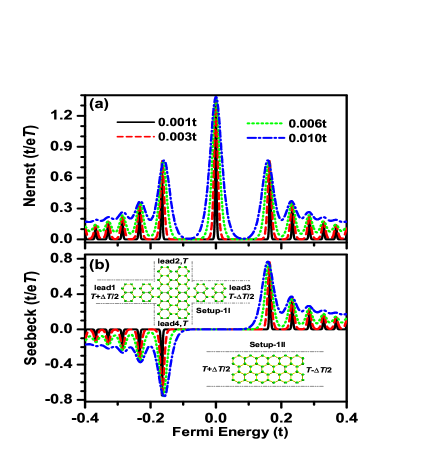
Figure 1: (Color online) Nernst coefficient $N_{C}$ (a) in the four terminal system and Seebeck coefficient $S_{C}$ (b) in two terminal system vs Fermi Energy $E_{F}$ with the strong magnetic field $BS_{0}=0.008\phi_{0}/\pi$ and ribbon width $N=80$. Different curves are for different temperatures $k_{B}\mathcal{T}$. The four terminal system and the two terminal system are shown in left and right inset in panel (b), respectively.

III.1 the strong perpendicular magnetic field case

Firstly, we study the system with strong perpendicular magnetic field. Fig.1 shows the Nernst coefficient $N_{C}$ and Seebeck coefficient $S_{C}$ versus Fermi energy $E_{F}$ for different temperatures $\mathcal{T}=0.001t$, $0.003t$, $0.006t$ and $0.01t$. Considering the ambipolar nature of the graphene and the electron-hole symmetry, the Nernst coefficient $N_{C}$ is an even function of $E_{F}$ [$N_{C}(E_{F})=N_{C}(-E_{F})$], because both the energy $E-E_{F}$ and the direction of the particle movement (or $T_{21}-T_{23}$) reverse their signs under the electron-hole transformation. From Fig.1(a), we see that the Nernst coefficient $N_{C}$ show peaks when $E_{F}$ passes the LLs $E_{n}=sign(n)\sqrt{2e\hbar v_{F}^{2}|n|B}$ and show valleys between adjacent LLs. With the increase of the temperature, the peak heights roughly remain unchanged, but the valleys rise. For convenience, the peaks are numbered and the peak at $E_{F}=0$ is denoted as the zeroth peak. In the low temperature limits, for the $n$-th peak with $n\not=0$, the height is $[\ln 2/|n|]$, and the zeroth peak height is $[2\ln 2]$. In Fig.2(a) we plot inverse of the peak heights versus the peak number $n$ (see the crossed circle symbols) at the low temperature $\mathcal{T}=0.001t$. It satisfies the relation $[|n|/\ln 2]$. For comparison, the inverse of the peak’s height for the conventional metal is also plotted (see dotted pentagram symbol), which is $[(n+1/2)/\ln 2]$.

In Fig.1(b), we plot the Seebeck coefficient $S_{C}$ versus $E_{F}$ at different temperatures $\mathcal{T}$. Similarly, the Seebeck coefficient $S_{C}$ display peaks when $E_{F}$ passes the LLs and show valleys between adjacent LLs. However, $S_{C}$ shows two essential differences from the Nernst effect: First, $S_{C}$ is an odd function of $E_{F}$, which means that contributions to $S_{C}$ from electrons and holes differ by a sign due to the electron-hole symmetry. So the Seebeck coefficient $S_{C}$ is negative for $E_{F}<0$. Second, when $E_{F}$ is on the zero-th LL, $S_{C}$ is zero instead of the highest peak in the curve of $N_{C}$-$E_{F}$. This is because the zero-th LL with the fourfold degeneracy is shared equally by electrons and holes and the electrons and holes give the opposite contributions to $S_{C}$. The inverse of the peak height of Seebeck coefficient at the low temperature ($k_{B}\mathcal{T}=0.001t$) is plotted in Fig.2(b). It is found that in graphene, the pseudospin related Berry phase ref01 introduces an additional phase shift in the magneto-oscillation of TEP. As a result of this phase shift, the inverse of peak height is $\propto n$ (see the crossed circle symbol in Fig.2(b)). While in the conventional metal or semiconductor with massive carriers, there is no pseudospin related berry phase, the inverse of peak height is $\propto n+\frac{1}{2}$ (see dotted pentacle symbol in Fig.2(b)).

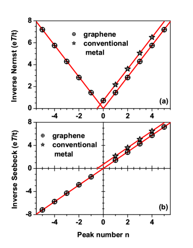
Figure 2: (Color online) The panel (a) and (b) are respectively the inverse of peak height of Nernst and Seebeck coefficients vs. the peak number $n$. The crossed circle symbols are for the graphene and dotted pentagram symbols are for the conventional metal. The temperature $k_{B}\mathcal{T}=0.001t$ and other parameters are the same as Fig.1. In panel (a), the two lines are $|n|/\ln 2$ and $(n+1/2)/\ln 2$ and in panel (b) the two lines are $n/\ln 2$ and $(n+1/2)/\ln 2$.

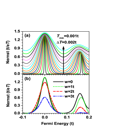
Figure 3: (Color online) Panel (a): the magnifications of the zeroth and first Nernst peaks in Fig.1(a). Along the arrow direction, temperature $k_{B}\mathcal{T}$ increases from $0.001t$ to $0.029t$ with increment of $0.002t$. Panel (b): the disorder effect of panel (a) at a fixed temperature $k_{B}\mathcal{T}=0.01t$.

Next, we study the temperature effect. Since TEP (Nernst effect or Seebeck effect) represents the entropy transported per unit charge, both Nernst coefficient and Seebeck coefficient increase with the increasing temperature which are exhibited in Fig.1(a) and (b). To take a closer look in Fig.3, we plot the zeroth and first peak for the temperature range $\in[0.001t,0.029t]$ in the step of $0.002t$. The temperature effect of $S_{C}$ is similar to that of $N_{C}$, so we only show the Nernst coefficient $S_{C}$ in Fig.3(a). At low temperatures, with the increase of the temperature $k_{B}\mathcal{T}$, the peak height and position do not vary much, but the peak half-width is broadened proportional to $k_{B}\mathcal{T}$, so the valley between the LLs rises. When the temperature $k_{B}\mathcal{T}$ exceeds the spacing of nearest LLs, the Nernst and Seebeck coefficients $N_{C}$ and $S_{C}$ are enhanced in the whole range of energies including both the peak and valley because of the overlap of the neighboring peaks. In addition, except for the zeroth peak, the peak positions for all other peaks shift towards the zeroth peak.

Now we study the disorder effect on the Nernst and Seeback effect. To consider the effect of disorder, random on-site potentials $\delta\epsilon_{i}$ in the center region are added with a uniform distribution $[-W/2,W/2]$ with disorder strength W. The data is obtained by averaging over up to 1200 disorder configurations. It is known that when the magnetic field is absent, the Seebeck effect is strongly affected by the disorder, and the peaks are suppressed even in the small disorder. On the other hand, in the presence of the strong magnetic field, the Seebeck effect and Nernst effect are robust to the disorder, because of the existence of the quantized Landau level. The bigger the sample is (or the stronger the magnetic field is), the more robust the Nernst effect and Seebeck effect. Similar to Fig.3(a), in Fig.3(b) we plot the zeroth and first peak at fixed temperature $k_{B}\mathcal{T}=0.01t$ with different disorder strengths. Here sample size ($N=40$) is smaller than that in Fig.1(a) (in which $N=80$). With the smaller sample size, the zeroth universal values of peak height $2\ln 2$ can still remain until disorder $W$ is larger than $1t$. For the first peak, the universal values of height $\ln 2/|n|$ remains at $W=0.3t$ and washes out at stronger disorder. It means that the Nernst peak corresponding to the lower Landauer level can resist stronger disorders. In fact, this effect of disorder has been studied for the thermal response to the charge currenttheory1 or to the spin current.Cheng So, in the following, we will focus only on the clean system.

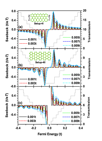
Figure 4: (Color online) Seebeck coefficient $S_{C}$ vs. Fermi energy $E_{F}$ for the different temperatures $k_{B}\mathcal{T}$ at zero magnetic field. Panel (a) is for the zigzag ribbon as sketched in the inset of panel (a), with the width $N=40$. Panel (b) and (c) are for the armchair ribbon sketched in inset of panel (b) with the width $N=41$ (b) and $N=40$ (c). The gray solid curves in panels (a), (b), and (c) are the corresponding transmission coefficients $T$.

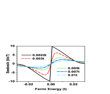
Figure 5: (Color online) The Seebeck coefficient of Fig.4(c) with the Fermi Energy interval $[-0.03,0.03]$.

III.2 the case of zero magnetic field

In this subsection, we study the TEP at zero magnetic field. Because there is no Lorentz force to bend the trajectories of the thermally diffusing carriers, the Nernst effect is absent and $N_{C}=0$. At $B=0$, the Seebeck coefficient $S_{C}$ is strongly dependent on the chirality of graphene ribbon. In addition, for the armchair edge ribbon, it is metallic when $N=3M-1$ ($M$ is an integer) and insulator otherwise.ref5 The Seebeck coefficient $S_{C}$ has essential difference for the metallic and insulator armchair ribbons. In the following we consider three different systems: (1) zigzag edge ribbon with width $N=40$ (sketched in inset of Fig.4(a)), (2) metallic armchair edge ribbon with width $N=41$ (sketched in inset of Fig.4(b)), and (3) insulating armchair edge ribbon with width $N=40$ (sketched in inset of Fig.4(b)). Fig.4(a), (b), and (c) show the Seebeck coefficient $S_{C}$ versus $E_{F}$ for the above three systems, respectively. For the convenience of discussion, we also plot corresponding transmission coefficient $T=T_{21}=T_{12}$ versus $E_{F}$ in each panel. We can see that $S_{C}$ is an odd function of $E_{F}$ and $S_{C}$ increases when the temperature increases. In addition, $S_{C}$ peaks when Fermi energy crosses the discrete transverse channels where quantized transmission coefficient jumps from one step to another. These properties are similar for the above three cases.

But there are also many essential different behaviors. (1). For the zigzag edge ribbon, the transverse channels are equidistance with the energy interval $\Delta=|t|\pi/(2N)$ in the conduction band or the valence band (except that the interval from the first transmission channel in the conduction band to the first transmission channel in the valence band is $3\Delta$). So peaks of $S_{C}$ are uniformly distributed over energies and the peak height of $S_{C}$ satisfies $[\ln 2/2n]$ where $n$ is the peak number (see Fig.4(a)). (2). In metallic armchair edge ribbon, however, the transverse channel and consequently the peaks of $S_{C}$ are irregularly distributed. The peak height of $S_{C}$ is closely related to the transmission coefficient $T=T_{21}=T_{12}$ and it can be expressed as $2\Delta Tln2/(2T+\Delta T)$ at low temperatures, where $\Delta T$ is the change of $T$ when $E_{F}$ scans over the certain transverse channel. With increasing of the temperature, some of peaks that are very close to each other merge together so that both peak height and position are irregular (see Fig.4(b)). (3). Finally, for the insulating armchair edge ribbon, except for the irregularly distributed peaks for $|E_{F}|>\Delta$, the Seebeck coefficient $S_{C}$ is very large for $E_{F}$ near the Dirac point (0) at low temperatures. Fig.5 magnifies the curves of $S_{C}$-$E_{F}$ near the Dirac point. At low temperatures, $S_{C}$ can be very large when $E_{F}$ approaches the Dirac point. For example $S_{C}$ can reach about $10$ at $\mathcal{T}=0.0022t$. At the Dirac point the sign of $S_{C}$ changes abruptly. This is because near the Dirac point the transmission coefficient $T_{12}$ is zero and the carriers can’t be transmitted. In order to balance the thermal forces acting on the charge carriers, we have to add a very large bias leading to a very large Seebeck coefficient near the Dirac point at low temperatures. When temperature increase such that $k_{B}\mathcal{T}$ is greater than the gap of the insulating armchair edge ribbon $S_{C}$ decreases gradually. We emphasize that if the armchair edge ribbon is narrow enough (such as $W\approx 10nm$ as in our calculation), $S_{C}\approx 10$ at the temperature $\mathcal{T}=0.0022t/k_{B}\approx 60K$. This very large $S_{C}$ can be observed in the present technology.

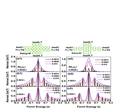
Figure 6: (Color online) Panel (a)-(c) plot the Nernst coefficient $N_{C}$ vs Fermi Energy $E_{F}$ at different temperatures $k_{B}\mathcal{T}=0.001t$, $0.005t$ and $0.01t$ in the magnetic field $BS_{0}=0.0005\phi_{0}/\pi,0.002\phi_{0}/\pi$ and $0.005\phi_{0}/\pi$, respectively. In left panels the thermal gradient is added along the zigzag edge ribbon as shown in the left top sketch. While in the right panels, the thermal gradient is added along the armchair edge ribbon as shown in the right top sketch. The ribbon width $N=80$.

III.3 the crossover from zero magnetic field to high magnetic field

In this subsection, we study the Nernst and Seebeck effect when the magnetic field varies from zero to finite values (strong magnetic field). At zero magnetic field, the Nernst coefficient $N_{C}$ is zero and the Seebeck effect $S_{C}$ is dependent on the chirality of graphene ribbon. At high magnetic fields, however, both $N_{C}$ and $S_{C}$ are independent of the ribbon chirality. What happens with the magnetic field in the intermediate range?

First, we study the Nernst effect, in which two different setups (the setup-6I and setup-6II) sketched in the top of Fig.6 are considered. In Fig.6 we plot the Nernst coefficient $N_{C}$ versus $E_{F}$ at different temperatures and magnetic fields. From Fig.6(a) to (c), the magnetic field increases from weak to strong enough to form edge state. At the weak magnetic field (such as $BS_{0}/\phi_{0}=0.0005/\pi$), the Nernst coefficient $N_{C}$ peaks sharply near the Dirac point at low temperatures. Because on two sides of the Dirac point, the carriers are electron-like and hole-like and they are shifted to the opposite direction under the weak magnetic field, the Nernst effect is largest at the Dirac point.

In particular, in the setup-6I, the Nernst coefficient $N_{C}$ is very large at the Dirac point, which is much larger than that in setup-6II and in the case of high magnetic field. Because for the setup-6I, the longitudinal leads (lead-1 and lead-3) are metallic with a large transmission coefficient but the transverse leads (lead-2 and lead-4) are almost insulator near the Dirac point. As a result, we have to add a much larger bias to balance the thermal current so that the Nernst coefficient $N_{C}$ is very large in the setup-6I at the low magnetic field (see Fig.6(a1) and (b1)). With increasing of $B$, LLs are formed one by one. The zeroth LL located at the Dirac point is formed first (at about $BS_{0}/\phi_{0}=0.0015/\pi$, no shown), then is the first LL, the second and so on. For example, In Fig.6(a), no LL is formed while in Fig.6(b), the zeroth, first and second LL are formed. As soon as LLs are formed, the Nernst coefficient $N_{C}$ will satisfy the relation that its peak heights are equal to $\ln 2/|n|$ (or $2\ln 2$ for $n=0$). From Fig.6(c), we can see that as $BS_{0}/\phi_{0}=0.005/\pi$, electrons (or holes) with Fermi energy $|E_{F}|\leq 0.3t$ all belong to robust edge states. In this case, the Nernst coefficient $N_{C}$ are almost the same for the setup-6I and setup-6II.

For the Seebeck effect, armchair edge ribbon can either be metal or insulator, we also consider three different systems as in the case of zero magnetic field. In Fig.7 we plot the Seebeck coefficient $S_{C}$ versus $E_{F}$ at different temperatures and magnetic fields for three different systems. The first column is for the zigzag edge ribbon with width $N=80$, the second column is for metallic armchair edge ribbon with $N=80$, and the third column is for insulating armchair edge ribbon with $N=81$. From Fig.7(a) to Fig.7(c), the magnetic field increases gradually. We can see that in the weak magnetic field, the peaks of $S_{C}$ are still regularly distributed for the zigzag ribbon and are irregular for the armchair ribbon due to the different band structure for the zigzag edge and armchair edge ribbon. Moreover, for the insulating armchair edge ribbon, the energy gap near Dirac point is diminished because of the magnetic field $B$, the very high and sharp $S_{C}$ at $B=0$ (see Fig.5) is gradually dropped with the increasing of $B$. But at the weak magnetic field $BS_{0}/\phi_{0}=0.0005/\pi$, the $N_{C}$ can still reach 3 (see Fig.7(a3)), which is much larger than all peaks of $S_{C}$ in the high magnetic field case. Similar to Fig.6, with the increasing of $B$ further, the LLs is gradually formed from Dirac point to the high $E_{F}$, the the properties of $S_{C}$ for three systems gradually tend to the same. At the high magnetic field $BS_{0}/\phi_{0}=0.005/\pi$, LLs are completely formed for $|E_{F}|<0.3$, then Seebeck coefficient $S_{C}$ for three different systems are all the same to that in the Hall region.

IV conclusion

In summary, by using the Landauer-B$\ddot{u}$ttiker formula combining with the non-equilibrium Green’s function method, the Nernst effect in the crossed graphene ribbon and the Seebeck effect in the single graphene ribbon are investigated. It is found that due to the electron-hole symmetry, the Nernst coefficient $N_{C}$ is an even function while the Seebeck coefficient $S_{C}$ is an odd function of the Fermi energy $E_{F}$. $N_{C}$ and $S_{C}$ show peaks when $E_{F}$ crosses the Landau levels at high magnetic fields or crosses the transverse sub-bands at the zero magnetic field. In the strong magnetic field, due to the fact that high degenerated Landau levels dominate transport processes the Nernst and Seebeck coefficients are similar for different chirality ribbons. The peak height of $N_{C}$ and $S_{C}$, respectively, are $[\ln 2/|n|]$ and $[\ln 2/n]$ with the peak number $n$, except for $n=0$. For zeroth peak, it is abnormal. Its peak height is $[2\ln 2]$ for the Nernst effect and it disappears for the Seebeck effect. While in zero magnetic field, Nernst effect is absent and the Seebeck effect is strongly dependent on the chirality of the ribbon. For the zigzag edge ribbon, the peaks of $S_{C}$ are equidistance, but they are irregularly distributed for armchair edge ribbon. Surprisingly, for the insulating armchair edge ribbon, the Seebeck coefficient $S_{C}$ can be very large near the Dirac point due to the energy gap. When the magnetic field increases from zero to high values, the irregularly or regularly distributed peaks of $S_{C}$ in different chiral ribbons gradually tends to be the same. In addition, the nonzero values of the Nernst coefficient $N_{C}$ appear first near the Dirac point and then gradually in the whole energy region. It is remarkable that for certain crossed ribbons, the Nernst coefficient $N_{C}$ at weak magnetic fields can be much larger than that in the strong magnetic field due to small transmission coefficient in the transverse terminals.

$${\bf ACKNOWLEDGMENTS}$$

We gratefully acknowledge the financial support by a RGC grant (HKU 704308P) from the Government of HKSAR and NSF-China under Grants Nos. 10525418, 10734110, and 10821403.

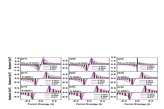
Figure 7: (Color online) Panel (a)-(c) plot the Nernst coefficient $N_{C}$ vs Fermi Energy $E_{F}$ at different temperatures $k_{B}\mathcal{T}$ and different magnetic fields $BS_{0}/\phi_{0}$. The other parameters and the chirality of ribbon for the first, second, and third column panels are the same as Fig.4(a), (b), and (c), respectively.

References

- (1) K.S. Novoselov, A.K. Geim, S.V. Morozov, D. Jiang, Y. Zhang, S.V. Dubonos, I.V. Grigorieva, and A.A. Firsov, Science 306, 666 (2004).
- (2) K.S. Novoselov, A.K. Geim, S.V. Morozov, D. Jiang, M.I. Katsnelson, I.V. Grigorieva, S.V. Dubonos, and A.A. Firsov, Nature (London) 438, 197 (2005); Y. Zhang, Y.-W. Tan, H.L. Stormer, and P. Kim, Nature (London) 438, 201 (2005).
- (3) C.W.J. Beenakker, Rev. Mod. Phys. 80, 1337 (2008); A.H. Castro Neto, F.Guinea ,N.M.R. Peres ,K.S. Novselov, and A.K. Geim, Rev. Mod. Phys. 81, 109 (2009).
- (4) J. R. Williams, L. Dicarlo and C. M. Marcus, Science 317, 638 (2008); A. f. Young and P. Kim, Nature Phys. 5, 222 (2009).
- (5) K. Nakada, M. Fujita, G. Dresselhaus and M. S. Dresselhaus, Phys. Rev. B 54, 17954 (1996).
- (6) K. Wakabayashi, M. Fujita, H. Ajiki and M. Sigrist, Phys. Rev. B 59, 8271 (1999);
- (7) V. P. Gusynin1, and S. G. Sharapov, Phys. Rev. B 73, 245411 (2006).
- (8) A. A. Abrikosov, Fundamentals of the Theory of Metals (North- Holland, Amsterdam, 1988); J. M. Iiman, Electrons and Phonons (Oxford University Press, Oxford, UK, 1960); C. W. J. Beenakker and A. A. M. Staring, Phys. Rev. B 46, 9667 (1992).
- (9) M. Cutler and N. F. Mott, Phys. Rev. 181, 1336 (1969); D. K. C. Macdonald, Thermoelectricity (Dover, New York, 2006).
- (10) A. S. Dzurak, C. G. Smith, C. H. W. Barnes, M. Pepper, L. Martín-Moreno, C. T. Liang, D. A. Ritchie, and G. A. C. Jones, Phys. Rev. B 55, R10197 (1997); R. Scheibner, H. Buhmann, D. Reuter, M. N. Kiselev, and L.W. Molenkamp, Phys. Rev. Lett. 95, 176602 (2005); R. Scheibner, E. G. Novik, T. Borzenko, M. König, D. Reuter, A. D. Wieck, H. Buhmann, and L. W. Molenkamp, Phys. Rev. B 75, 041301 (2007).
- (11) H.-C. Ri, R. Gross, F. Gollnik, A. Beck, R. P. Huebener, P. Wagner and H. Adrian, Phys. Rev. B 50, 3312 (1994); C. Hohn, M. Galffy and A. Freimuth, Phys. Rev. B 50, 15875 (1994); Z. A. Xu, J. Q. Shen, S. R. Zhao, Y. J. Zhang and C. K. Ong, Phys. Rev. B 72, 144527 (2005);
- (12) S. Onoda, N. Sugimoto, and N. Nagaosa, Phys. Rev. B 77, 165103 (2008); Wei-Li Lee, S. Watauchi, V. L. Miller, R. J. Cava, and N. P. Ong, Phys. Rev. Lett. 93, 226601 (2004); T. Miyasato, N. Abe, T. Fujii, A. Asamitsu, S. Onoda, Y. Onose, N. Nagaosa, and Y. Tokura, Phys. Rev. Lett. 99, 086602 (2007).
- (13) A. Banerjee, B. Fauque, K. Izawa, A. Miyake, I. Sheikin, J. Flouquet, B. Lenoir and K. Behnia, Phys. Rev. B 78, 161103(R) (2008).
- (14) N. Hanasaki, K. Sano, Y. Onose, T. Ohtsuka, S. Iguchi, I. Kzsmrki, S. Miyasaka, S. Onoda, N. Nagaosa and Y. Tokura, Phys. Rev. Lett. 100, 106601 (2008).
- (15) K. Behnia, M. A. Masson, and Y. Kopelevich, Phys. Rev. Lett. 98, 166602 (2007); K. Behnia, L. Balicas, Y. Kopelevich, Science 317, 1729 (2007).
- (16) Joshua P. Small, Kerstin M. Perez, and Philip Kim, Phys. Rev. Lett. 91, 256801 (2003).
- (17) Y. M. Zuev, W. Chang, and P. Kim, Phys. Rev. Lett. 102, 096807 (2009).
- (18) P. Wei, W. Bao, Y. Pu, C. N. Lau, and J. Shi, Phys. Rev. Lett. 102, 166808 (2009).
- (19) M. Cutler and N. F. Mott, Phys. Rev. 181, 1336 (1969); D. K. C. Macdonald, Thermoelectricity (Dover, New York, 2006).
- (20) N. M. R. Peres, J. M. B. Lopes dos Santos and T. Stauber, Phys. Rev. B 76, 073412 (2007).
- (21) B. Dóra and P. Thalmeier, Phys. Rev. B 76, 035402 (2007).
- (22) H. Nakamura, N. Hatano, and R. Shirasaki, Solid State Commun. 135, 510 (2005).
- (23) R. Shirasaki, H. Nakamura, and N. Hatano, e-J. Surf. Sci. Nanotechnol. 3, 518 (2005).
- (24) M. Jonson and S. M. Girvin, Phys. Rev. B 29, 1939 (1984); H. Oji and P. Streda, Phys. Rev. B 31, 7291 (1985); J. Phys. C: Solid State Phys., 17, 3059 (1984)-3066.
- (25) D. N. Sheng, L. Sheng, and Z. Y. Weng, Phys. Rev. B 73, 233406 (2006); Z. Qiao and J. Wang, Nanotechnology 18, 435402 (2007).
- (26) W. Long, Q.-F. Sun, and J. Wang, Phys. Rev. Lett. 101, 166806 (2008); J. Li and S.-Q. Shen, Phys. Rev. B 78, 205308 (2008).
- (27) In the references, [M. Jonson and S. M. Girvin, Phys. Rev. B 29, 1939 (1984) and H. Oji and P. Streda, Phys. Rev. B 31, 7291 (1985)], they pointed out that the standard Kubo formula can’t apply to the Nernst coefficient in the presence of strong magnetic fields, because that a diamagnetic surface currents and a “diathermal” surface currents appear under the strong mangetic fields. So a fundamental correction on the standard Kubo formula is necessary. However, the Landauer-Buttiker formula is to calculate the current flowing from a terminal to the center region, in which the both interior and surface currents have been included. So it is validity regardless of the magnetic field.
- (28) D. H. Lee and J. D. Joannopoulos, Phys. Rev. B 23, 4997 (1981); ibid, 23, 4988 (1981).
- (29) S.-G Cheng, Y. Xing, Q.-F Sun and X. C. Xie, Phys. Rev. B 78, 045302 (2008).