Breaking the $Z_{2}$ symmetry of the Randall-Sundrum scenario
and the fate of the massive modes

Abstract

We address in detail the issue of possible resonances in the massive modes on a brane without reflection symmetry. After identifying a set of solvability conditions, we show explicitly how the modes of the asymmetric case can be traced back to the modes of the symmetric RS-2 scenario. The possible occurrence of resonances is revisited and discussed by finding analytical solutions. We find that the resonant behavior is very mild even for strong asymmetries, and moreover it occurs only for very large masses, so that its effects on the Newtonian potential are exponentially suppressed.

General considerations. The set-up for the Randall-Sundrum scenario of Ref.Randall:1999vf (RS-2 scenario) is a single 3-brane with positive tension embedded in a $AdS_{5}$ space with reflection symmetry along the extra dimension. The problem of a single 3-brane embedded in a $AdS_{5}$ space without reflection symmetry, i.e. with different cosmological constants $\Lambda_{+}$ and $\Lambda_{-}$ in each side, has been considered in Melfo:2002wd ; Castillo-Felisola:2004eg ; Gabadadze:2006jm ; Guerrero:2006gj . In Ref.Castillo-Felisola:2004eg , this asymmetric scenario arises (rigorously) as the thin wall limit of a self-gravitating thick domain wall spacetime generated by a topologically non-trivial scalar field configuration, and the Newtonian potential is shown to be the usual one: a dominant four dimensional term due to a massless bound state, plus small corrections due to the massive modes. Some properties of the asymmetric scenarios have been discussed in Melfo:2002wd ; Castillo-Felisola:2004eg ; Gabadadze:2006jm ; Guerrero:2006gj ; Padilla:2004tp ; Padilla:2004mc ; Koyama:2005br ; Guerrero:2005aw ; Bogdanos:2007ti ; Bazeia:2007nd ; Liu:2009dw . In particular, the occurrence of resonances related to the asymmetry has been put forward in Gabadadze:2006jm .

Technically, the evaluation of the contribution of the Kaluza-Klein (KK) modes to the Newtonian potential on the brane requires an explicit knowledge of the graviton wavefunction and, in order to quantize the system, regulator (negative tension) branes are introduced. In the RS-2 scenario, due to the assumed reflection symmetry and hence with the fifth dimension compactified on an orbifold $S_{1}/Z_{2}$, we have two branes that represent the boundaries of the fifth dimension. At the end of the calculation, the regulator brane is taken to infinity and a non-compact fifth dimension is thus obtained. The techniques employed to obtain the KK modes in the RS-2 symmetric scenario can be extended to the asymmetric case without modifications. The evaluation of these modes is, however, not as straightforward as in the $Z_{2}$-symmetric case, since the symmetry to characterize this modes is no longer at our disposal. Additionally, it may be difficult to fix their normalization, which is crucial to get the correct relative contribution from the zero mode as compared to the massive ones in the gravitational Newtonian potential on the brane. Given the current interest in asymmetric scenarios as brane-worlds, a careful derivation of the massive modes is then in order. Since a thorough discussion of this problem leads to certain solvability conditions which must be satisfied, let us first revisit in some detail the evaluation of the KK modes in the RS-2 scenario.

KK modes in the symmetric scenario. Let us consider the metric of the RS-2 scenario in conformal coordinates

$$g_{ab}=e^{2A(z)}\left(\eta_{\mu\nu}\,dx^{\mu}_{a}dx^{\nu}_{b}+dz_{a}dz_{b}\right),$$ (1)

where $A(z)=-\ln(1+k|z|)$ and $\eta_{\mu\nu}=\mathrm{diag}(-1,1,1,1)$. In order to find the KK expansion of the graviton modes we parametrize the graviton fluctuation in the standard way

$$g_{ab}=e^{2A(z)}\left((\eta_{\mu\nu}+h_{\mu\nu})\,dx^{\mu}_{a}dx^{\nu}_{b}+dz_{a}dz_{b}\right),$$ (2)

and define $h_{\mu\nu}=e^{ip\cdot x}e^{A(z)/2}\psi_{\mu\nu}(z)$, so that $\psi_{\mu\nu}$ satisfies the Schrödinger equation

$$\left(-\frac{d^{2}}{dz^{2}}+V_{QM}\right)\psi_{\mu\nu}(z)=m^{2}\psi_{\mu\nu}(z),\qquad-\infty<z<\infty,$$ (3)

with

$$V_{QM}=\frac{15}{4}\frac{k^{2}}{(1+k|z|)^{2}}-3k\delta(z).$$ (4)

Integration of (3,4) across the brane, $\psi_{\mu\nu}$ being continuous, yields

$$\psi_{\mu\nu}(0^{+})=\psi_{\mu\nu}(0^{-}),\qquad\frac{d}{dz}\psi_{\mu\nu}(0^{+})-\frac{d}{dz}\psi_{\mu\nu}(0^{-})=-3k\,\psi_{\mu\nu}(0).$$ (5)

(we shall omit the indices $\mu,\nu$ from now on). For $m^{2}=0$ the solution of (3, 4) is well-known to be $\psi_{0}(z)=N_{0}e^{3A(z)/2}$, with $N_{0}$ a normalization constant.

Let us focus on the massive modes. How many nontrivial solutions does (3,4) have? Let $\varphi(z)=\psi_{m}(z)/\psi_{m}(0)$, with $\psi_{m}(0)\neq 0$. Since the difference between two solutions $\varphi_{1}(z)$ and $\varphi_{2}(z)$ of (3,4) associated to the same eigenvalue $m^{2}$ has a continuous first derivative everywhere, this difference is the classical solution $\psi_{m}^{clas}(z)$ of

$$\left(-\frac{d^{2}}{dz^{2}}+\frac{15}{4}\frac{k^{2}}{(1+k|z|)^{2}}\right)\psi_{m}^{clas}(z)=m^{2}\psi_{m}^{clas}(z),\qquad\psi_{m}^{clas}(0)=0,\qquad-\infty<z<\infty.$$ (6)

Following a procedure close to the one employed to obtain Green’s functions for the general self-adjoint problem of the second order Stakgold , the condition $\psi_{m}^{clas}(0)=0$ can be related to the solvability condition that ensures that the (regularized) problem is consistent and that every solution of (3,4) can then be written as an arbitrary linear combination of $\psi_{m}^{dist}(z)$ and $\psi_{m}^{clas}(z)$, where $\psi_{m}^{dist}(z)$ is any particular solution that carries all the singular information (5) and $\psi_{m}^{clas}(z)$ is the classical solution of (6). Of course, in (3), the symmetry condition $V_{QM}(z)=V_{QM}(-z)$ has the consequence that for every $m^{2}$ there exist solutions of even and odd parity. Since the even solution incorporates the distributional solution, the odd solution is therefore the classical one. Being automatically orthogonal to each other,

$$(\psi^{o}_{m},\psi^{e}_{m})=\int_{-\infty}^{\infty}dz\,\,\psi_{m}^{o}(z)^{*}\,\psi_{m}^{e}(z)=0,$$ (7)

these even (or distributional) and odd (or classical) functions appropriately normalized are the two ortonormal modes associated to the same eigenvalue $m^{2}$, which is therefore degenerate.

The modes should be normalized by requiring

$$(\psi_{m^{\prime}},\psi_{m})=\int_{-\infty}^{\infty}dz\,\,\psi_{m^{\prime}}(z)^{*}\,\psi_{m}(z)=\delta(m-m^{\prime}).$$ (8)

However, since the integral in (8) is divergent $\forall\,m,m^{\prime}$, some regularization procedure is required.

Following Randall:1999vf (see Callin:2004py for a detailed derivation), we introduce regulator (negative tension) branes at $\pm z_{r}$ taking the limit $z_{r}\rightarrow\infty$ at the end and the resulting scenario will be called the regularized one. Now the gravitational fluctuations satisfy the additional integrability conditions

$$\psi_{m}(z_{r}^{+})=\psi_{m}(z_{r}^{-}),\qquad\frac{d}{dz}\psi_{m}(z_{r}^{+})-\frac{d}{dz}\psi_{m}(z_{r}^{-})=\frac{3}{2}\frac{k}{1+kz_{r}}\psi_{m}(z_{r}),$$ (9)

and these conditions quantize the mass spectrum in units of $\pi/z_{r}$. Now (8) reads as

$$\int_{-z_{r}}^{z_{r}}dz\,\psi_{m_{p}}(z)^{*}\psi_{m_{q}}(z)=\delta_{pq}.$$ (10)

The corresponding density of states is used to evaluate the Newtonian potential, which is then given by Randall:1999vf ; Callin:2004py

$$V_{N}(r)=\frac{1}{4\pi M^{3}}\frac{m_{1}m_{2}}{r}\left[|\psi_{0}(0)|^{2}+\frac{4}{3\pi}\sum_{i=1}^{2}\int_{0}^{+\infty}dm\,{|\psi_{m}^{i}(0)|^{2}e^{-mr}}z_{r}\right]\;\;,$$ (11)

where $M$ is the $5$-dimensional Planck mass.

Solutions for the even modes are the best known, as they appear in the symmetric case. For $m^{2}\neq 0$ the solution is given by

$$\psi_{m}^{e}(z)=N_{m}^{e}(k^{-1}+|z|)^{1/2}\left\{Y_{2}[m(k^{-1}+|z|)]-\frac{Y_{1}(mk^{-1})}{J_{1}(mk^{-1})}J_{2}[m(k^{-1}+|z|)]\right\},$$ (12)

where $J_{n}(x)$ and $Y_{n}(x)$ are the Bessel functions of order $n$ of the first and second kind, respectively, and $N_{m}^{e}$ is a normalization constant determined by (10). Setting $m_{p}=m_{q}=m$ we have

$$(2z_{r}(N_{m}^{e})^{2})^{-1}=\frac{1}{z_{r}}\int_{0}^{z_{r}}dz\,(k^{-1}+z)\left\{Y_{2}[m(k^{-1}+z)]-\frac{Y_{1}(mk^{-1})}{J_{1}(mk^{-1})}J_{2}[m(k^{-1}+z)]\right\}^{2}$$ (13)

and we obtain by making use of the asymptotics of the Bessel functions

$$(N^{e}_{m})^{2}=\frac{\pi m}{2z_{r}}\left[1+\frac{Y_{1}^{2}(mk^{-1})}{J_{1}^{2}(mk^{-1})}\right]^{-1}.$$ (14)

Let us now consider the odd massive modes. For $m^{2}\neq 0$ the odd solution of (3,4) is given by

$$\psi_{m}^{o}(z)=N^{o}_{m}(k^{-1}+z)^{1/2}\left\{Y_{2}[m(k^{-1}+z)]-\frac{Y_{2}(mk^{-1})}{J_{2}(mk^{-1})}J_{2}[m(k^{-1}+z)]\right\},\qquad z>0\,,$$ (15)

with $\psi_{m}^{o}(z)=-\psi_{m}^{o}(-z)$, $z<0$, and with $N_{m}^{o}$ a normalization constant in the Dirac’s sense of eq. (8). Since $\psi_{m}^{o}(z)$ has a zero at the brane’s position, $\psi_{m}^{o}(0)=0$, as follows from (5) their derivative is continuous at $z=0$ and, as expected, the odd solutions are unaffected by the brane.

We stress that the odd modes have to be normalized by introducing the usual regulator branes. The boundary conditions at $z=\pm z_{r}$ turn the continuous spectrum of masses into a discrete one with even and odd modes sharing the same mass spectrum for $z_{r}\rightarrow\infty$. However, in the symmetric scenario the odd massive modes do not contribute to the Newtonian potential at the brane located at $z=0$ and we obtain the Newtonian potential of Ref.Randall:1999vf (see also Callin:2004py ).

The asymmmetric case. Next, let us consider the spectrum of gravitational fluctuations of the asymmetric scenario Castillo-Felisola:2004eg ; Gabadadze:2006jm ; Guerrero:2006gj . Here, where the gravitational fluctuations satisfy a Schrödinger equation which is not invariant under $z\leftrightarrow-z$, the massive modes are not functions of definite parity. Instead of odd and even modes, we will have weak and distributional ones. The weak modes will play a key role in determining in a consistent way the distributional modes that contribute to the gravitation on the brane. Since this point seems to be taken lightly on previous works, we will go through the calculations in some detail.

Let $g_{ab}$ be the metric given by (1) with

$$A(z)=-\Theta(-z)\ln(1-k_{-}z)-\Theta(z)\ln(1+k_{+}z),$$ (16)

where $k_{+}$ and $k_{-}$ are related to the cosmological constants $\Lambda_{+}$ and $\Lambda_{-}$ at the sides of the brane by $k_{\pm}=\sqrt{-\Lambda_{\pm}/6}$. It was shown that (1,16) can be associated to the metric of an asymmetric BPS domain wall spacetime Castillo-Felisola:2004eg , in the distributional thin wall limit Guerrero:2002ki .

Now $V_{QM}$ is given by

$$V_{QM}=\frac{15}{4}\,\frac{k_{-}^{2}}{(1-k_{-}z)^{2}}\,\Theta(-z)+\frac{15}{4}\,\frac{k_{+}^{2}}{(1+k_{+}z)^{2}}\,\Theta(z)-\frac{3}{2}(k_{-}+k_{+})\,\delta(z).$$ (17)

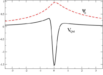
Figure 1: $V_{QM}$ and the (arbitrarily normalized) zero-mode red$\psi_{0}$ for $k_{-}>k_{+}>0$, with a regularized $\delta$.

As with (3,4), the solution of (3,17) can be written as an arbitrary linear combination of a distributional solution $\psi^{dist}_{m}(z)$, which carries the singular information

$$\psi^{dist}_{m}(0^{+})=\psi^{dist}_{m}(0^{-})=\psi^{dist}_{m}(0)\neq 0,\qquad\frac{d}{dz}\psi^{dist}_{m}(0^{+})-\frac{d}{dz}\psi^{dist}_{m}(0^{-})=-\frac{3}{2}(k_{-}+k_{+})\psi^{dist}_{m}(0),$$ (18)

and a weak solution $\psi^{w}_{m}(z)$, such that $\psi^{w}_{m}(0^{+})=\psi^{w}_{m}(0^{-})=\psi^{w}_{m}(0)=0$, with a continuous first derivative everywhere and therefore not affected by the presence of the brane. Although $\psi_{m}^{w}$ is not strictly a classical solution, since $\lim_{z\rightarrow 0^{+}}V_{QM}\neq\lim_{z\rightarrow 0^{-}}V_{QM}$, the condition $\psi_{m}^{w}(0)=0$ can still be related to the solvability condition that ensures that the (regularized) problem is consistent Stakgold .

For $m^{2}=0$ there exists a distributional solution $\psi_{0}(z)=N_{0}e^{3A(z)/2}$, with $A(z)$ given by (16) and gravity is localized on the brane since $\psi_{0}(z)$ can be normalized, with $N_{0}$ given by

$$N_{0}=\sqrt{2}\left[k_{-}^{-1}+k_{+}^{-1}\right]^{-\frac{1}{2}}.$$ (19)

Fig. 1 shows the shape of $V_{QM}$ and the zero mode.

For $m^{2}\neq 0$, the weak solution is given by

$$\psi^{w}_{m}(z)=N^{w}_{m}\begin{cases}+k_{+}^{-1/2}(k_{+}^{-1}+z)^{1/2}\left[J_{2}(mk_{+}^{-1})Y_{2}(m(k_{+}^{-1}+z))-Y_{2}(mk_{+}^{-1})J_{2}(m(k_{+}^{-1}+z))\right],&z>0\cr&\cr-k_{-}^{-1/2}(k_{-}^{-1}-z)^{1/2}\left[J_{2}(mk_{-}^{-1})Y_{2}(m(k_{-}^{-1}-z))-Y_{2}(mk_{-}^{-1})J_{2}(m(k_{-}^{-1}-z))\right],&z<0\cr\end{cases}$$ (20)

where $N_{m}^{w}$ is a normalization constant to be found later.

It should be stressed that the weak solution (20) is unique, up to a multiplicative constant $N_{m}^{w}$, while a distributional solution is one of an infinite set of particular solutions of (3,17,18) since, as follows from the solvability condition $\psi_{m}^{w}(0)=0$, any linear combination of (20) and a particular solution of (3,17,18) is also a solution of (3,17,18). In absence of $Z_{2}$ symmetry, $\psi^{w}_{m}(z)$ and a particular $\psi^{dist}_{m}(z)$, although linearly independent solutions, are not automatically orthogonal and can not be identified a priori with the orthonormal massive modes associated to $m^{2}$, a fact that has been overlooked in some previous works Guerrero:2006gj ; Bogdanos:2007ti . This should not be a problem since in a regularized scenario, a Gram-Schmidt process may be used to convert an independent set into an orthonormal set with the same span. In the following, the regularization procedure of the previous section will be considered.

Introducing regulator branes at $\pm z_{r}$, where the limit $z_{r}\rightarrow\infty$ will be taken at the end of the calculations, the gravitational fluctuations satisfy (3) but with $V_{QM}(z)$ given by

$$V_{QM} = \frac{15}{4}\,\Theta(-z)\,\Theta(z_{r}+z)\frac{k_{-}^{2}}{(1-k_{-}z)^{2}}+\frac{15}{4}\,\Theta(z)\,\Theta(z_{r}-z)\,\frac{k_{+}^{2}}{(1+k_{+}z)^{2}}$$ (21)

$$-\frac{3}{2}(k_{-}+k_{+})\,\delta(z)+\frac{3}{2}\left[\frac{k_{-}}{1+k_{-}z_{r}}\,\delta(z+z_{r})+\frac{k_{+}}{(1+k_{+}z_{r})}\delta(z-z_{r})\right],$$

which imposes on $\psi_{m}(z)$ the integrability conditions at $z=\pm z_{r}$

$$\psi_{m}(z_{r}^{+})=\psi_{m}(z_{r}^{-}),\qquad\frac{d}{dz}\psi_{m}(z_{r}^{+})-\frac{d}{dz}\psi_{m}(z_{r}^{-})=\frac{3}{2}\frac{k_{+}}{1+k_{+}z_{r}}\psi_{m}(z_{r}),$$ (22)

$$\psi_{m}(-z_{r}^{+})=\psi_{m}(-z_{r}^{-}),\qquad\frac{d}{dz}\psi_{m}(-z_{r}^{+})-\frac{d}{dz}\psi_{m}(-z_{r}^{-})=\frac{3}{2}\frac{k_{-}}{1+k_{-}z_{r}}\psi_{m}(-z_{r}).$$ (23)

As in the previous section, these conditions turn the continuous spectrum of massive modes into a discrete spectrum.

An analogous calculation to that of (14) leads to

$$(N_{m}^{w})^{2}=\frac{\pi m}{z_{r}}\left[k_{-}^{-1}\left(Y_{2}^{2}(mk_{-}^{-1})+J_{2}^{2}(mk_{-}^{-1})\right)+k_{+}^{-1}\left(Y_{2}^{2}(mk_{+}^{-1})+J_{2}^{2}(mk_{+}^{-1})\right)\right]^{-1}.$$ (24)

Next, to obtain the distributional mode $\psi_{m}^{dist}$ which is orthonormal to $\psi_{m}^{w}$, we find the solution of (3,21) requiring additionally that

$$(\psi_{m}^{dist},\psi_{m}^{w})_{z_{r}}\doteq\lim_{z_{r}\rightarrow\infty}\int_{-z_{r}}^{z_{r}}dz\,\psi_{m}^{dist}(z)^{*}\psi_{m}^{w}(z)=0,$$ (25)

which is evaluated making use of the asymptotics of the Bessel functions. This provides one and only one solution, up to a multiplicative constant, which after normalization also in the regularized scenario gives the desired orthonormal mode. We find

$$\psi^{dist}_{m}(z)=N^{dist}_{m}\begin{cases}(k_{-}^{-1}-z)^{1/2}\left[AY_{2}(m(k_{-}^{-1}-z))+BJ_{2}(m(k_{-}^{-1}-z))\right],&z<0\cr&\cr(k_{+}^{-1}+z)^{1/2}\left[CY_{2}(m(k_{+}^{-1}+z))+DJ_{2}(m(k_{+}^{-1}+z))\right],&z>0\cr\end{cases}$$ (26)

where

$$\left.\begin{array}[]{c}A=+{k_{-}^{\frac{1}{2}}\left[J_{1}^{-}\left[({Y_{2}^{+}})^{2}+({J_{2}^{+}})^{2}\right]+Y_{2}^{-}\left[J_{1}^{+}Y_{2}^{+}-J_{2}^{+}Y_{1}^{+}\right]+J_{2}^{-}\left[J_{1}^{+}J_{2}^{+}+Y_{1}^{+}Y_{2}^{+}\right]\right]}\;,\\ B=-{k_{-}^{\frac{1}{2}}\left[Y_{1}^{-}\left[({Y_{2}^{+}})^{2}+({J_{2}^{+}})^{2}\right]+J_{2}^{-}\left[J_{2}^{+}Y_{1}^{+}-J_{1}^{+}Y_{2}^{+}\right]+Y_{2}^{-}\left[J_{1}^{+}J_{2}^{+}+Y_{1}^{+}Y_{2}^{+}\right]\right]}\;,\\ C=+{k_{+}^{\frac{1}{2}}\left[J_{1}^{+}\left[({Y_{2}^{-}})^{2}+({J_{2}^{-}})^{2}\right]+Y_{2}^{+}\left[J_{1}^{-}Y_{2}^{-}-J_{2}^{-}Y_{1}^{-}\right]+J_{2}^{+}\left[J_{1}^{-}J_{2}^{-}+Y_{1}^{-}Y_{2}^{-}\right]\right]}\;,\\ D=-{k_{+}^{\frac{1}{2}}\left[Y_{1}^{+}\left[({Y_{2}^{-}})^{2}+({J_{2}^{-}})^{2}\right]+J_{2}^{+}\left[J_{2}^{-}Y_{1}^{-}-J_{1}^{-}Y_{2}^{-}\right]+Y_{2}^{+}\left[J_{1}^{-}J_{2}^{-}+Y_{1}^{-}Y_{2}^{-}\right]\right]}\;,\end{array}\right.$$ (27)

with $Y_{n}^{\pm}=Y_{n}(mk_{\pm}^{-1})$, $J_{n}^{\pm}=J_{n}(mk_{\pm}^{-1})$ and

$$(N_{m}^{dist})^{2}=\frac{\pi m}{z_{r}}\left[A^{2}+B^{2}+C^{2}+D^{2}\right]^{-1}.$$ (28)

Resonances. We are now ready to discuss resonances in this scenario. In Fig. 2, the value of $|\psi_{m}^{dist}|^{2}$ on the brane ($z=0$) is plotted for different values of the asymmetry. As is expected on general grounds from the shape of $V_{QM}$ (see Fig. 1), a resonance type behavior is observed. Although for strong asymmetries it becomes enhanced, this is nevertheless a very mild resonance. For larger values of $k_{+}$ and $k_{-}$, it occurs at very high masses, making its contribution to the Newtonian potential (11) negligible. Let us define $\eta=k_{+}/k_{-}\leq 1$. The mass of the resonance, defined as the location of the maximum of $|\psi_{m}^{dist}(0)|^{2}$, its approximately given by $\sqrt{k_{-}k_{+}}$ for $\eta\lesssim 0.4$. On the other hand, as follows from (19), the strength of the zero mode on the brane decreases for strong asymmetries.

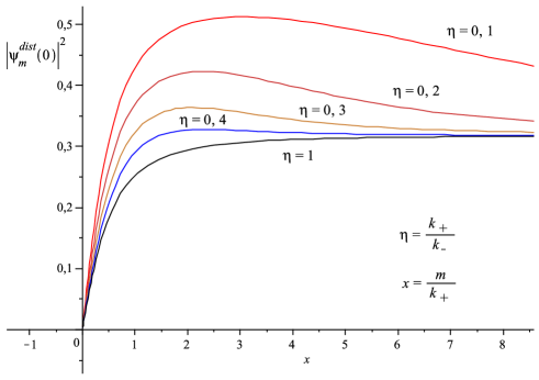
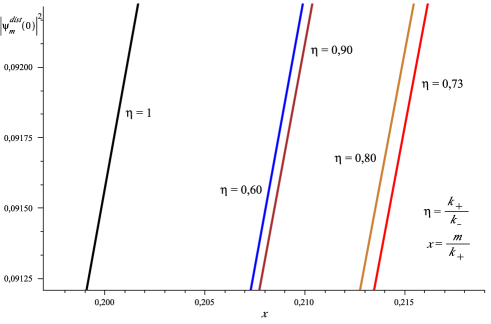
Figure 2: $|\psi_{m}^{dist}(0)|^{2}$ for different values of the ratio $\eta=k_{+}/k_{-}$ as a function of $x=m/k_{+}$.

For $m\ll k_{+}$, from (11) and (26,27,28), we find that the Newtonian potential in the asymmetric scenario is given by

$$V_{N}(r) \simeq \frac{m_{1}m_{2}}{2\pi M^{3}}\frac{k_{-}k_{+}}{r(k_{-}+k_{+})}\left[1+\frac{2(k_{+}^{2}-k_{-}k_{+}+k_{-}^{2})}{3k_{-}^{2}k_{+}^{2}}\left[\frac{1}{r^{2}}+\left.\frac{6}{r^{4}(k_{-}+k_{+})k_{-}^{2}k_{+}^{2}}\right[k_{-}^{3}\ln{(2k_{+}r)}+k_{+}^{3}\ln{(2k_{-}r)}\right.\right.$$ (29)

$$\left.\left.\left.-\frac{11}{6}(k_{-}^{3}+k_{+}^{3})+\frac{k_{-}^{5}+k_{+}^{5}}{2(k_{+}^{2}-k_{-}k_{+}+k_{-}^{2})}\right]\right]\right]+\mathcal{O}\left(\frac{1}{r^{7}}\right).$$

It follows that we have a four dimensional behavior of the Newtonian gravitational potential up to distances $r\sim 10^{2}\mu m$, even for arbitrarily large asymmetries, as far as $\text{min}\{k_{-},k_{+}\}\gg 10^{2}$ cm^-1. As expected, for $k_{-}=k_{+}=k$, the Newtonian potential in the $Z_{2}$-symmetric RS-2 scenario Randall:1999vf ; Callin:2004py is recovered. From (29), we find that the contribution of the massive tower of modes to the term $\sim r^{-3}$ of $V_{N}$ has a minimum for $\eta=\sqrt{3}-1$. Hence, there are slightly asymmetric scenarios in which the contribution of the massive modes to $V_{N}$ is weaker than in the $Z_{2}$-symmetric scenario while, as follows from FIG. 2, for strong asymmetries the contribution of these modes grows with the asymmetry.

The occurrence of resonances in the asymmetric scenario, as well as the weakness of the zero mode and the strength of the resonance for strong asymmetries, have been advanced in Gabadadze:2006jm , where a sharp resonance behavior for $m=m_{res}\sim\sqrt{k_{-}k_{+}}$ appears in one of two modes, being both scattered by the brane. It should be noted that in Gabadadze:2006jm , a normalization condition is adopted which is reduced to the standard one only for $k_{-}=k_{+}$. From these modes, the gravitational potential on the brane is then calculated numerically and compared to that of the $Z_{2}$-symmetric RS-2 scenario with $k^{-1}=(k_{+}^{-1}+k_{+}^{-1})/2$, finding that they differ the most at scales $r\sim m^{-1}_{res}=1/\sqrt{k_{+}k_{-}}$, and is argued that this result shows that these resonances may contribute appreciably to the Newtonian potential on the brane Gabadadze:2006jm . Since the very same result is obtained from (29), which however receives no contribution from masses $m\sim\sqrt{k_{+}k_{-}}$, it follows that the largest contribution to $V_{N}$ of the massive modes in the asymmetric scenario with respect to the RS-2 symmetric scenario should be traced back to the asymmetry, and not to the existence of the resonance.

The question naturally arises as to whether (3,21) can have solutions with a clear resonance behavior as in Gabadadze:2006jm , so we shall elaborate a little further on the choice of modes. Indeed, any pair $\psi_{m}^{1}$, $\psi_{m}^{2}$, of orthonormalized linear combinations of $\psi_{m}^{dist}$ and $\psi_{m}^{w}$, can be taken also as the massive modes in the asymmetric scenario. However, in the absence of additional symmetries, any other choice of modes different from the orthonormal set $\psi_{m}^{dist}$, $\psi_{m}^{w}$, is arbitrary and therefore devoid of physical meaning. Let us consider the following example, which shows explicitly this arbitrariness. Let $\psi_{m}^{1}$, $\psi_{m}^{2}$ be given by

$$\psi_{m}^{1}(z)=\frac{1}{\sqrt{1+c^{2}}}\left(\psi_{m}^{w}(z)+c\,\psi_{m}^{dist}(z)\right),\qquad\psi_{m}^{2}(z)=\frac{1}{\sqrt{1+c^{2}}}\left(-c\,\psi_{m}^{w}(z)+\psi_{m}^{dist}(z)\right),$$ (30)

where $c$ is a constant which depends arbitrarily on $m$, $k_{-}$ and $k_{+}$, and $\psi_{m}^{dist}$, $\psi_{m}^{w}$ are given by (26,27,28) and (20,24), respectively. The set $\{\psi_{m}^{1},\psi_{m}^{2}\}$ is an orthonormal set, in the regularized scenario, of solutions of (3,21). Now, we have

$$|\psi_{m}^{1}(0)|^{2}=\frac{c^{2}}{1+c^{2}}|\psi_{m}^{dist}(0)|^{2},\qquad|\psi_{m}^{2}(0)|^{2}=\frac{1}{1+c^{2}}|\psi_{m}^{dist}(0)|^{2},$$ (31)

whose shapes depend on $c$. For instance, we can choose the constant $c$ such that $c\rightarrow 0$ for $k_{-}\rightarrow k_{+}$ and hence $\psi_{m}^{1}(z)\rightarrow\psi_{m}^{o}$ and $\psi_{m}^{2}(z)\rightarrow\psi_{m}^{e}$ as $k_{-}\rightarrow k_{+}$, where $\psi_{m}^{o}$ and $\psi_{m}^{e}$ are the odd and even modes of the $Z_{2}$ symmetric scenario. In any event, a sharp resonance type behavior in one of these modes is an artifact introduced by an, up to some extent, arbitrary descomposition as (30). Nevertheless, since

$$|\psi_{m}^{1}(0)|^{2}+|\psi_{m}^{2}(0)|^{2}=|\psi_{m}^{dist}(0)|^{2},$$ (32)

this decomposition gives exactly the same contribution to the Newtonian potential on the brane (11) as the original set $\{\psi_{m}^{dist},\psi_{m}^{w}\}$.

Discussion. We have shown that the calculation of the Newtonian potential arising in asymmetric RS-2 scenarios requires a careful identification of the orthonormal massive modes associated with each value of $m^{2}$. By normalizing these modes in the standard way, we have revisited the calculations of Gabadadze:2006jm . Our analytical solutions show that the resonant behavior is indeed present, but that it is extremely mild and has no significant contribution to the Newtonian potential. We have shown that the main effect in the Newtonian potential arises not from the resonances, but from the asymmetry itself. Hence, for a wide range of asymmetries, the asymmetric scenario is essentially on the same footing as the original symmetrical one, in terms of the effective 4-dimensional gravitational potential on the brane.

References

(1)
L. Randall and R. Sundrum,
Phys. Rev. Lett. 83, 4690 (1999)
[arXiv:hep-th/9906064].
(2)
A. Melfo, N. Pantoja and A. Skirzewski,
Phys. Rev. D 67 (2003) 105003
[arXiv:gr-qc/0211081].
(3)
O. Castillo-Felisola, A. Melfo, N. Pantoja and A. Ramirez,
Phys. Rev. D 70 (2004) 104029
[arXiv:hep-th/0404083].
(4)
G. Gabadadze, L. Grisa and Y. Shang,
JHEP 0608 (2006) 033
[arXiv:hep-th/0604218].
(5)
R. Guerrero, A. Melfo, N. Pantoja and R. O. Rodriguez,
Phys. Rev. D 74 (2006) 084025
[arXiv:hep-th/0605160].
(6)
A. Padilla,
Class. Quant. Grav. 22 (2005) 681
[arXiv:hep-th/0406157].
(7)
A. Padilla,
Class. Quant. Grav. 22 (2005) 1087
[arXiv:hep-th/0410033].
(8)
K. Koyama and K. Koyama,
Phys. Rev. D 72 (2005) 043511
[arXiv:hep-th/0501232].
(9)
R. Guerrero, R. O. Rodriguez and R. S. Torrealba,
Phys. Rev. D 72 (2005) 124012
[arXiv:hep-th/0510023].
(10)
C. Bogdanos, A. Dimitriadis and K. Tamvakis,
Class. Quant. Grav. 25 (2008) 045008
[arXiv:0706.1015 [hep-th]].
(11)
D. Bazeia, A. R. Gomes and L. Losano,
Int. J. Mod. Phys. A 24 (2009) 1135
[arXiv:0708.3530 [hep-th]].
(12)
Y. X. Liu, C. E. Fu, L. Zhao and Y. S. Duan,
Phys. Rev. D 80 (2009) 065020
[arXiv:0907.0910 [hep-th]].
(13)
P. Callin and F. Ravndal,
Phys. Rev. D 70 (2004) 104009
[arXiv:hep-ph/0403302].
(14)
R. Guerrero, A. Melfo and N. Pantoja,
Phys. Rev. D 65, 125010 (2002)
[arXiv:gr-qc/0202011].
(15)
I. Stakgold, Green’s functions and boundary value problems
(Wiley-Interscience, New York, 1979).