Supersolid in a one-dimensional optical lattice in the presence of a harmonic trap

Abstract

We study a system of ultra-cold atoms possessing long range interaction (e.g. dipole-dipole interaction) in a one dimensional optical lattice in the presence of a confining harmonic trap. We have shown that for large enough on-site and nearest neighbor interaction a supersolid phase can be stabilized, consistent with the previous Quantum Monte Carlo and DMRG results for the homogeneous system. Due to the external harmonic trap potential the supersolid phase coexists with other phases. We emphasize on the experimental signatures of the various ground state phases in the presence of a trap.

I INTRODUCTION

The realization of the supersolid form of matter, where the superfluid and the crystalline order co-exist andreev ; legget , in the ultra-cold bosonic atoms in optical lattices is at the forefront of research. After the claim of observing the supersolid phase in solid ${}^{4}He$ by Kim et al chan , the progress in the research of this exotic phase of matter has advanced substantially. The successful observation of the superfluid (SF) to Mott insulator (MI) transition in ultra-cold bosonic atoms in $3D$ bloch and subsequently in $2D$ spielman and $1D$ stoferle has shaped the study of ultra-cold systems as an ideal tool to understand condensed matter phenomena. In order to achieve the supersolid form of matter that is characterized by the co-existence of the superfluid and crystalline order, it is essential for the system to have long range interactions. The remarkable experimental realization of BEC in $Cr$ atoms pfau that have fairly large dipole moment, has increased the expectations to observe the supersolid phase in optical lattice experiments.

In recent years there have been several theoretical evidences for the supersolid phase in various lattice geometries batrouniprl ; mishrass ; kedar ; arun ; sengupta ; wessel ; scarola . However, the experimental search of the supersolid in the ultra-cold atomic systems in optical lattices still remains a challenge. The real experimental situation is different from the usual homogeneous system considered in theoretical calculations. In experiments, the translational symmetry of the lattice is broken due to the presence of an external harmonic trap potential (magnetic or optical) and various quantum phases co-exist  wessel1 ; svistunov ; bergkvist ; pollet ; smita ; mitra ; spiel ; nandini ; suna ; batrounimi . Hence, it is essential to understand the signatures of the supersolid phase in the presence of such a trap.

In this paper we have considered a system of ultra-cold bosonic atoms possessing long range interactions in a one dimensional optical lattice with a harmonic confinement. The Hamiltonian for this kind of system is represented by the extended Bose-Hubbard model,

$$H = -t\sum_{<i,j>}(a_{i}^{\dagger}a_{j}+H.c)+\frac{U}{2}\sum_{i}n_{i}(n_{i}-1)$$ (1)

$$\mbox{}+V\sum_{<i,j>}n_{i}n_{j}+V_{\text{T}}\sum_{i}\,r_{i}^{2}n_{i}.$$

Here, $t$ is the hopping amplitude between the nearest neighbor sites $\langle i,j\rangle$, $a_{i}^{\dagger}(a_{i})$ is the bosonic creation (annihilation) operator obeying the Bosonic commutation relation $[a_{i},a_{j}^{\dagger}]=\delta_{i,j}$ and $n_{i}=a_{i}^{\dagger}a_{i}$ is the number operator. $U$ and $V$ are the on-site and the nearest neighbor interactions, respectively. $V_{\text{T}}$ is the magnitude of the external trap potential and $r_{i}$ is the distance from the trap center. We re-scale in units of the hopping amplitude, $t$, setting $t=1$, making the Hamiltonian and other quantities dimensionless.

The homogeneous version of this model (i.e. without the external trap), has been studied earlier using several techniques in one dimension mishrass ; pai ; whiteprb ; batrouniprl ; kashurnikov ; batrouni95 ; niyaz ; kuhner ; iskin . The prediction of an accurate phase diagram using Quantum Monte Carlo method batrouniprl and DMRG mishrass has revealed the physical conditions required to stabilize a supersolid phase. It has been shown that the supersolid phase is obtained when:

1. The total density of the system is incommensurate to the lattice.

2. The on-site ($U$) and the nearest neighbor interactions ($V$) are fairly large compared to the hopping amplitude ($t$).

3. The condition $U<2V$ is satisfied.

A homogeneous system exhibits a uniform phase determined by the global chemical potential for a given set of interaction parameters. The phase diagram of the model in Eq. 1 in the homogeneous limit i.e., $V_{\text{T}}=0$, exhibiting different possible phases including the supersolid phase is shown in Fig. 2 mishrass .

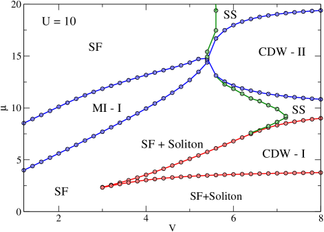
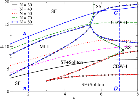
Figure 1: (Color on line) The phase diagram of the model in Eq. 1 in the homogeneous limit i.e., $V_{\text{T}}=0$ and for $U=10.0$ in the $\mu-V$ plane.

Figure 2: (Color on line) Homogeneous phase diagram for the model in Eq. 1 showing canonical trajectories. For a given value of $V$, the presence of an external trap allows all phases that fall on the line that starts from the canonical trajectory to the V-axis for example: lines AB and CD in the figure.

In the presence of an external trap, the role of a local chemical potential becomes important as demonstrated in our earlier work on the Bose-Hubbard model suna . Since the local chemical potential varies from the center of the trap to the edges, the system exhibits different phases simultaneously. An earlier DMRG study of model given in Eq. 1 could not confirm the presence of the supersolid phase in the system urba . A recent study of this model in two dimension using mean field theory predicts that the noise correlation could be a valid signature to separate the supersolid phase from the other ground state phases scarola . In this paper we re-visit the extended Bose-Hubbard model with the external harmonic trap potential and search for experimental signatures of the different ground state phases, in particular, the supersolid phase.

The remaining part of the paper is organized as follows. In Sec. II, we discuss the method of our calculation using the finite size density matrix renormalization group (FS-DMRG) technique. The results along with discussions are presented in Sec. III with experimental signatures for the different ground state phases in Sec. IV and we present our conclusions in Sec. V.

II METHOD OF CALCULATION

To obtain the ground state of model (1) for the system of $N$ bosons on a lattice of length $L$, we use the FS-DMRG method with open boundary conditions white ; schollwock . This method has been widely used to study the Bose-Hubbard model pai ; kuhner ; whiteprb ; schollwock ; urba . We have considered six bosonic states per site and the weights of the states neglected in the density matrix formed for the left or the right blocks are less than $10^{-6}$ pai . In order to improve the convergence of the results, the finite-size sweeping procedure as given in white ; pai has been used for every length. Using the ground state wave function $|\psi_{LN}\rangle$ and energy $E_{L}(N)$, we calculate the following physical quantities and use them to identify the different phases.

The on-site local number density $\langle n_{i}\rangle$, defined as,

$$\langle n_{i}\rangle=\langle\psi_{LN}|n_{i}|\psi_{LN}\rangle,$$ (2)

gives the local density distribution. The fluctuation in the local number density, $\kappa_{i}$, which is finite for the SF phase, is calculated using the relation

$$\kappa_{i}=\langle{n_{i}^{2}}\rangle-{\langle{n_{i}}\rangle}^{2}$$ (3)

and finally the existence of the CDW order is confirmed by calculating the structure factor:

$$S(k)=\frac{1}{L^{2}}\sum_{i,j}e^{i\,k\,(i-j)}\langle{n_{i}n_{j}}\rangle.$$ (4)

In our calculations, we have considered a system of length $L=140$ and vary $N$ from $30$ to $140$. In our previous work on the homogeneous extended Bose-Hubbard Model mishrass , we had considered a fixed value of the on-site interaction $U=10$ and vary the nearest neighbor interaction strengths $V$ from $0$ to $10$. We choose the same range of parameters here as well, since the homogeneous phase diagram for this range, as shown in the Fig. 2, exhibits most of the interesting phases for this model. The strength of the external confining trap potential is fixed at $V_{\text{T}}=0.008$.

III Results and Discussion

We begin with the summary of the phase diagram for the homogeneous extended Bose-Hubbard model, which has been studied recently batrouniprl ; mishrass for a wide range of densities and interaction parameters namely, the on-site interaction $U$ and the nearest neighbor interaction $V$. The phase diagram for a typical value of the on-site interaction, say $U=10$ is shown in Fig. 2 mishrass . The phase diagram consists of gapped as well as gapless phases. The gapless phases include the superfluid phase, the supersolid phase where superfluidity and charge density wave order co-exist, and the solitonic phases. The gapped phases are (i) the Mott insulator phase with $\rho=1$ for $V<V_{C}\sim 5.4$, (ii) charge density wave phase CDW-II, (where every other site is doubly occupied, i.e., $|2~{}0~{}2~{}0~{}\cdots\rangle$) with average density $\rho=1$ for $V>V_{C}\sim 5.4$ and (iii) the CDW-I phase (alternative sites are occupied, i.e., boson density varies as $|1~{}0~{}1~{}0~{}\cdots\rangle$) with average density $\rho=1/2$ for $V>V_{C}\sim 3.0$. The gap vanishes when doping above or below these gapped phases. For example doping below half-filling ($\rho=1/2$) gives rise to solitons that break the CDW-I order. This phase extends over a small range of densities below the CDW-I and eventually goes over to the superfluid phase when the density is further decreased. However, the behavior of the system when doping above half-filling is different. For small $V$ we get similar solitonic phases, however, for larger $V$ a supersolid phase stablizes. The supersolid phase forms again while doping above and below the CDW-II phase. In fact there exists a range densities $0.5<\rho<1$ and $\rho>1$ for $V>U/2$ where the supersolid phase is the stable ground state of model (1) as shown in the Fig. 2.

Let us introduce a harmonic trap potential. Earlier studies of the one-dimensional Bose-Hubbard model in the presence of a trap has demonstrated the co-existence of the superfluid and the Mott insulator phases suna ; batrounimi . The Mott insulator is characterized by the formation of a plateau in the local number density $\langle n_{i}\rangle$ as a function of the distance $r_{i}$ from the center of the trap and is incompressible, while the superfluid phase is characterized by large local number density fluctuations and is compressible. The nearest neighbor interaction brings about the charge density wave order in the system due to the interplay between the $U$ and $V$ terms in the Hamiltonian. Figures 3 and 4 show the density profile, i.e., the variation of the local density $\langle n_{i}\rangle$ as a function of the distance from the trap center $r_{i}$. We obtain the density profile for two sets of parameters: (i) for the number of bosons fixed at $N=80$, but different values of $V$ (Fig. 3) and (ii) fixed nearest neighbor interaction, $V=8$, but different values of $N$ (Fig. 4). The following three features are clearly seen: (i) the local density $\langle n_{i}\rangle$ is maximum at the center of the trap, (ii) the density falls-off with increase in $r_{i}$ and (iii) the density profile exhibits plateaus and oscillations.

In order to understand these features and identify various phases from the density profile, we define the local chemical potential at the site $i$ at a distance $r_{i}$ from the center of the trap as,

$$\mu_{i}=\mu_{0}-V_{\text{T}}r_{i}^{2}.$$ (5)

Here $\mu_{0}=E_{L}(N+1)-E_{L}(N)$ is the chemical potential of the system. For the homogeneous system, $\mu_{i}=\mu_{0}$ for any $i$. However, for a finite trap the local chemical potential $\mu_{i}$ equals $\mu_{0}$, which is its maximum value, at the center of the trap and decreases radially outward as in Eq. 5. It is instructive to plot the density profile as a function of $\mu_{i}$ instead of $r_{i}$ as in Fig. 5. It may be noted from Fig. 5 that the density of bosons at any site $i$ is controlled by the value of the local chemical potential $\mu_{i}$. So a decrease in $\mu_{i}$ results in a decrease in $\langle n_{i}\rangle$, with the maximum at the center of the trap as observed in Figs. 3 and 4.

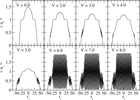
Figure 3: The local density $\langle n_{i}\rangle$ as a function of the distance from the center of the trap $r_{i}$ for $N=80$, $U=10$, $V_{\text{T}}=0.008$, but for different values of $V$.

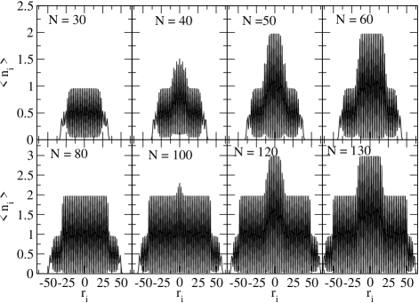
Figure 4: The local density $\langle n_{i}\rangle$ as a function of the distance from the center of the trap $r_{i}$ for fixed $V=8$, $U=10$, $V_{\text{T}}=0.008$, but for different values of $N$.

The density of bosons plays a very crucial role in the determination of the ground state of the model in Eq. 1. The gapped phases are possible only when the density is commensurate. The homogeneous system with a given value of $U$ and $V$ and a uniform local chemical potential $\mu_{0}$ represents one point in the phase diagram. However, for the system with a trap potential, the density varies across the lattice due to the variation of the local chemical potential and therefore different phases co-exist. In order to understand this feature of co-existence of the different ground state phases and the role played by the local chemical potential, we study first the path in the phase diagram that is traced by $\mu_{0}$ as we change the interaction parameter $V$ keeping the number of bosons $N$, the trap potential $V_{T}$ and the on-site interaction $U$ fixed. This path is referred to as the Canonical Trajectory batrounimi , since $N$ is held fixed. Fig. 2 shows several canonical trajectories (for different values of $N$) in the homogeneous phase diagram. In may be noted that $\mu_{0}$ is the local chemical potential at the center of the trap and the position of these canonical trajectories trace the phase present at the trap center as $V$ is varied for fixed $N$. For example when $N=30$, the canonical trajectory and hence the phase at the center of the trap goes from the superfluid to CDW-I as we increase $V$. The position of the canonical trajectory in the phase diagram can be shifted by changing the number of bosons $N$. When the number of bosons is increased, say to $N=40$, $\mu_{0}$ increases and the position of the canonical trajectory in the phase diagram is shifted upward. As a result the center of the trap, say for $V=0$, which was in the SF phase for $N=30$, is now in the Mott insulator phase. Following the canonical trajectory for $N=40$, the trap center goes from MI to SF and then to a supersolid phase for increasing $V$. Thus the position of the canonical trajectory for a given $N$ and $V$ in the phase diagram represents the phase at the center of the trap.

Moving away from the center of the trap, the local chemical potential decreases as in Eq. (5) and the variation of $\mu_{i}$ is represented in the phase diagram by a line drawn vertically downwards from the canonical trajectory to the horizontal axis. The local chemical potential values across the lattice fall on this line, which passes through different ground state phases. Therefore, the local chemical potential (and thus local density) at different sites favor the co-existence of different phases in the presence of a trap. It is useful to re-plot the density profile given in the Fig. 3 as a function of $\mu_{i}$ using Eq. 5 instead of $r_{i}$ as in Fig. 5. We also calculate and plot, in the same figure, the average local number density define as

$$\bar{n}_{i}=\langle(2n_{i}+n_{i+1}+n_{i-1})\rangle/4.$$ (6)

For $N=80$ and $V=2.0$, $\mu_{0}$ falls in the superfluid phase above the $\rho=1$ Mott lobe (point $A$ as indicated on the canonical trajectory corresponding to $N=80$ in Fig 2). This means that the center of the trap has $\langle n_{i}\rangle>1$. Moving away from the trap center, $\mu_{i}$ decreases along the line $AB$ and there are regions where $\mu_{i}$ falls inside the MI lobe. From Fig. 5, we see that for these values of $\mu_{i}$, $\langle n_{i}\rangle=1$. Similarly as we move towards the edge, the values of $\mu_{i}$ decreases further such that the system is once again in a superfluid phase on the lower side of the Mott lobe. So the system for $N=80$, $V=2$ has a superfluid core flanked by a MI phase and finally ending with a superfluid edge. The density profile (top panel of Fig 3 and Fig 5) correlates with this result. In addition, there are oscillations in $\langle n_{i}\rangle$ in the superfluid shoulders near $\bar{n}_{i}=1/2$. The reasons for these oscillation are the following. For $V=2$, the system is close to CDW-I lobe (see Fig 2). In the thermodynamic limit, the CDW-I order can stabilize only for $V>V_{C}\sim 3.0$. However, the finite size of the system allows a CDW-I phase to exist for lower values of $V$, here $V=2$, although it vanishes in the thermodynamic limit. Finite size effects are characterized by oscillations in the local density $\langle n_{i}\rangle$. These oscillations stabilize at higher values of $V$ into the CDW-I phase. For example for $V=7$ and $N=80$, $\mu_{0}$ (point $C$ in Fig. 2) falls inside the CDW-II lobe yielding a CDW-II phase at the center. As we move towards the edges, the CDW-II phase is flanked by a supersolid phase, CDW-I and finally a superfluid shoulder as can also be infered from the density profiles as shown in Fig. 3 and Fig 5. In fact, these conclusions can be further fortified by comparing the variation of the average $\bar{n}_{i}$ as a function of $\mu_{i}$ with the density of the corresponding homogeneous system as in Fig. 6. The agreement is striking, leading to the conclusion that for a given set of parameters, the phase of a system with an external trap is represented by a line starting from the canonical trajectory to the horizontal axis while the phase of the homogeneous system is represented by a point in the phase diagram. This immediately shows that while the homogeneous system can have a unique phase, the phases tend to co-exist for an inhomogeneous system.

In addition to scanning along the phase diagram at fixed values of $N$ and varying $V$, it is also equally possible to fix the nearest neighbor interaction $V$ and move along the phase diagram by varying $N$ and therefore the chemical potential $\mu_{0}$. The canonical trajectory in the phase diagram moves upwards (downwards) by increasing (decreasing) the total number of bosons and as a result the local chemical potential at the center of the trap $\mu_{0}$ changes, giving rise to different phases at the center. This is demonstrated in Fig. 4 for fixed $V=8$ for different values of $N$. For $N=30$, position of the $\mu_{0}$ is inside the CDW-I lobe (see Fig. 2) and as discussed above, the corresponding system has a CDW-I core flanked by a superfluid edge as seen in the density profile (top panel of Fig. 4). An interesting situation occurs for $N=40$, where the trap center is expected to be in the elusive supersolid phase, as seen in Fig. 2 and is characterized by density fluctuations between $1.0\leq\langle n_{i}\rangle\leq 1.5$, that is, the system has a CDW order at incommensurate densities mishrass . As a result, the system now will have a supersolid core, followed by a CDW-I and a superfluid phase moving outward from the trap center (top panel of Fig. 4). Further increase in $N$ leads to the inclusion of a CDW-II phase in the system in addition to the supersolid, the CDW-I and the superfluid phases.

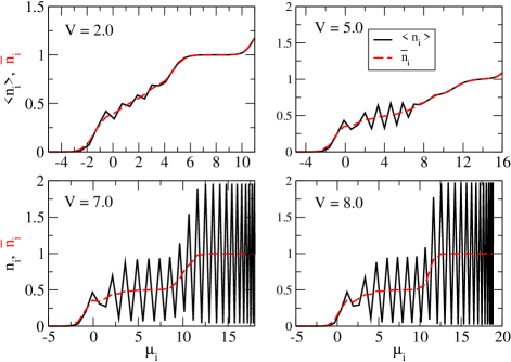
Figure 5: (Color on-line) Local number density $\langle n_{i}\rangle$ and average define as $\bar{n}_{i}=\langle(2n_{i}+n_{i+1}+n_{i-1})/4\rangle$ as a function of local chemical potential for different values of $V$ but fixed $N=80$.

Figure 6: (Color on-line) Average local number density $\bar{n}_{i}$ for system with a trap and $\langle n_{i}\rangle$ for a homogeneous system as function of the local chemical potential $\mu_{i}$ for $V=2$ and $7$.

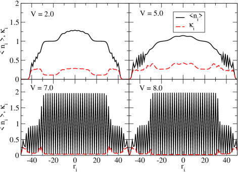
Figure 7: (Color on-line) Number density per site and its fluctuations that serve as a measure of compressibility and hence can be used as a tool to pick out the compressible and the incompressible phases that coexist in the presence of a harmonic trap.

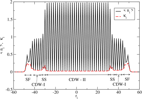
Figure 8: (Color on-line) Picking out the different phases from the density profile for $N=80$ and $V=8.0$.

The next issue we address here is a scheme to pick out the various phases using local properties of the system. We will follow the discussions in suna and use local compressibility or equivalently the fluctuations in the number density per lattice site, $\kappa_{i}$, given in Eq. 3, as a tool to distinguish between the gapped and the gapless phases. It is known that the number fluctuation is large in the superfluid phase while it is a minimum for the MI and the CDW phases. Fig. 7 shows the variation of $\kappa_{i}$ across the lattice. For small values of $V$, $\kappa_{i}$ varies at the center and at the edges of the trap indicating that these regions are in the superfluid phase, while the plateaus represent the Mott insulator phase. Further, we note that these plateaus (minima) occur exactly over the values of $r_{i}$ where the average local density $\bar{n}_{i}$ exhibits a plateau at integer densities. Therefore, one can pick out the incompressible phases using the density profile and its local fluctuation $\kappa_{i}$ and identify them using the phase diagram and the canonical trajectories. As an example, Fig. 8 shows the different phases for $N=80$ but varying $V$. In the next section, we will discuss the experimental signatures for the various phases that have been isolated in the presence of a harmonic trap using global properties of the system.

IV Experimental Signatures

The presence of a harmonic trap in the optical lattice leads to the co-existence of the superfluid, the Mott insulator, the charge density wave and the supersolid phases as seen in the previous sections. As a result, extracting the signature of a particular phase in the presence of other phases becomes a theoretically important exercise in order to make connections with experiments. In the following we analyze possible global signatures of the various ground state phases that can be experimentally confirmed.

It is now possible in experiments to record the spatial distribution of the lattice with different filling factors bloch06 ; gemelke ; sherson ; bakr . Similar experiments in one-dimensional optical lattices can yield density profiles using which the ground state phases can be mapped. Another way to obtain direct information about the Mott plateaus (shells in 3D) is through the atomic clock shift experiment campbel . By using density dependent transition frequency shifts, sites with different occupation can be spectroscopically distinguished, thus giving us information about the number of sites corresponding to a given density $\rho$ of bosons, defined as $N(\rho)$. As a first step, we look for the signatures of the solid phases (MI and CDW) in an atomic clock shift experiment.

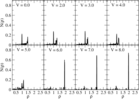
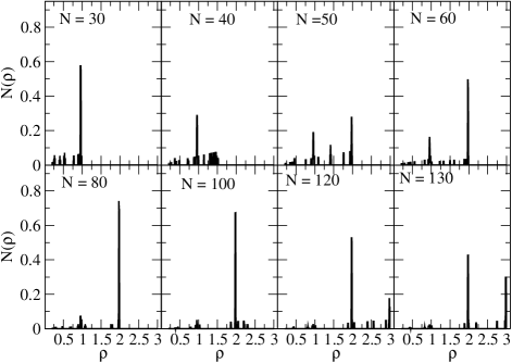
Figure 9: $N(\rho)$ versus $\rho$ for $N=80$ and different values of the nearest neighbor interaction $V$. The presence of incompressible phases can be distinguished by the formation of a peak at commensurate densities.

Figure 10: $N(\rho)$ versus $\rho$ for $V=8.0$ as number of Bosons is varied. Incompressible phases can be picked out by the formation of peaks at commensurate densities.

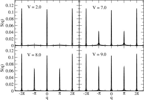
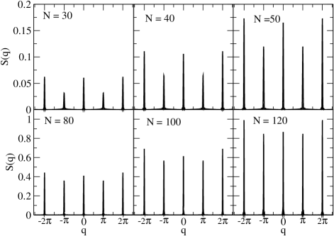
Figure 11: Structure factor as a function of $q$ for $N=40$ and different values of $V$.

Figure 12: Structure factor as a function of $q$ for $V=8.0$ and different values of $N$.

In Figs. 10 and 10 we plot $N(\rho)$ as a function of $\rho$ for different values of $V$ fixing $N=80$ and different $N$ values with fixed $V=8$ respectively. The density profiles corresponding to these parameter values are given in the Figs. 3 and 4 respectively. The presence of the incompressible phases, that is, the MI, the CDW-I and II in the system can be inferred from the formation of a peak in $N(\rho)$ at commensurate densities. For example, existence of a Mott plateau in the density profile for $V$ ranging between $0$ and $5$ ( see Fig 3) correlates with a peak in $N(\rho)$ at $\rho=1$. Similarly peaks in $N(\rho)$ at $\rho=2$ correlate with the formation of CDW-II phases in the density profile. Similar conclusions can be drawn from Fig 10. Comparing with the density profile in Fig 4, we can conclude that the formation of peaks in $N(\rho)$ at integer densities can be correlated with the existence of the solid phases, i.e., MI or CDW.

In order to distinguish between the two solid phases, i.e, the CDW and MI phase, we calculate the structure factor, as defined in Eq. 4. Fig. 12 shows the structure factor in momentum space as $V$ is varied for $N=40$, while Fig. 12 has fixed $V=8.0$ for different $N$ values. From the phase diagram (see the canonical trajectory in Fig. 2) for $N=40$ the phases at low $V$ values are the superfluid and the Mott insulator. However, for higher values of $V$, a CDW-I phase is possible. The CDW oscillations in the density profile translates to the formation of a peak at $q=\pi$ in the structure factor. As $V$ increases, this peak at $q=\pi$ grows in magnitude reaching its maximum value when the trap center exhibits the CDW crystalline structure. However this crystalline structure is possible for a CDW or a SS phase. For example, for $N=40$ and $V=8.0$, the center of the trap is in the supersolid phase that has the CDW-like crystalline structure and is compressible like a superfluid. Hence the next step is to distinguish between the CDW ordered phases that could be either compressible (SS phase) or incompressible (CDW phase itself). While this can be established locally with the behavior of compressibility as a function of the distance from the trap center, a global signature that can be used to check for the presence of a SS phase in the trap is the momentum distribution $n(q)$ scarola-demler-das .

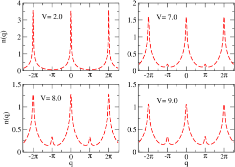
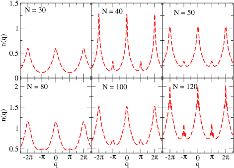
Figure 13: (Color on-line) Momentum distribution as a function of $q$ for $N=40$ and different values of $V$.

Figure 14: (Color on-line) Momentum distribution as a function of $q$ for $V=8.0$ and different values of $N$.

In experiments, the bosons in the optical lattice are allowed to expand and the interference pattern in the density is recorded. The density distribution is mirrored in the momentum distribution defined as,

$$n(q)=\displaystyle\frac{1}{L}\sum_{k,l=1}^{L}\langle a_{k}^{\dagger}a_{l}\rangle\exp(iq(k-l))$$ (7)

which then provides global information about the various phases present in the system. Figures 14 and 14 show the momentum distribution, respectively, for various values of $V$ with fixed $N=40$ and for various values of $N$ with fixed $V=8.0$. We see that in addition to the peaks at $q=0$ and $q=\pm 2\pi$, there are peaks around $q=\pi$. In order to understand the reason for this peak at $q=\pi$, let us look at the momentum distribution for the homogeneous system as in Fig. 16. We choose four densities to demonstrate the features of the peak in $n(q)$ at $q=\pi$. From the phase diagram we see that for $V=8.0$ the homogeneous system with $\rho=0.42$ is in the superfluid phase, $\rho=1/2$ and $1$ are, respectively, in CDW-I and CDW-II phases and for $\rho=0.67$, the system is in the supersolid phase. From Fig. 16 we note that the presence of a supersolid order in the system is accompanied by a peak in the momentum distribution at $q=\pi$, which is absent in the SF, CDW-I and CDW-II phases. The structure function for the same set of densities as given in Fig. 16 show peak at $q=\pi$ when the system is in CDW-I, CDW-II and SS phases. This confirm that the peak in $n(q)$ at $q=\pi$ is a clear signature of the supersolid phase.

Therefore for the trapped systems, when the phases co-exist, we note that a peak in the momentum distribution function at $q=\pi$ signals the presence of a supersolid phase somewhere in the trap, and the peak height being maximum when the supersolid occupies the center of the trap. We summarize below the signatures of the different ground state phases for the inhomogeneous extended Bose-Hubbard model:

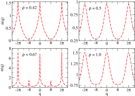
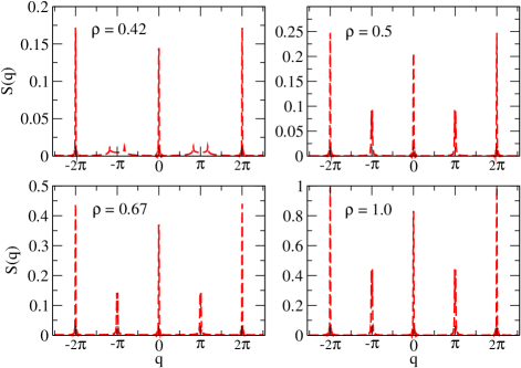
Figure 15: (Color on line) Momentum distribution for homogeneous case. Note that when the system is in the Supersolid phase, a peak at $q=\pi$ develops.

Figure 16: (Color on line) Structure function for homogeneous case. Note that when the system is in the Supersolid phase, a peak at $q=\pi$ develops.

• MI - Phase:

  • Peaks in $N(\rho)$ at integer densities.

  • No peaks in the momentum distribution at $n(q=\pi)$.

  • No peaks in the structure function at $S(q=\pi)$.

• CDW Phase:

  • Peaks in $N(\rho)$ at integer densities.

  • No peaks in the momentum distribution at $n(q=\pi)$.

  • Peaks in the structure function at $S(q=\pi)$.

• supersolid phase:

  • No Peaks in $N(\rho)$ at integer densities.

  • Peaks in the momentum distribution at $n(q=\pi)$

  • Peaks in the structure function at $S(q=\pi)$

V Conclusion

In conclusion, we have studied a system of dipolar ultra-cold bosonic atoms in the frame work of the extended Bose-Hubbard model in the presence of external harmonic trap. Using finite size density matrix renormalization group (FS-DMRG) method we have demonstrated the simultaneous existence of different phases in the system. We show the signature of different phases by calculating different observable quantities such as the on-site number density, the number fluctuation, the structure factor and the momentum distribution. We also document global signatures for the ground phases that can be observed experimentally.

VI Acknowledgement

R. V. P. acknowledges financial support from CSIR and DST, India.

References

- (1) A. F. Andreev and I. M. Lifshitz, Sov. Phys. JETP 29, 1107 (1969).
- (2) A. J. Leggett, Phys. Rev. Lett. 25, 1543 (1970).
- (3) E. Kim and M. H. W. Chan, Nature (London) 427, 225 (2004); Science 305, 1941 (2004).
- (4) M Greiner, O. Mandel, T. Esslinger, T. W. Ha nsch and I. Bloch, Nature 415, 39 (2002).
- (5) I. B. Spielman, W. D. Phillips, and J.V. Porto, Phys. Rev. Lett. 98, 080404 (2007).
- (6) T. Stöferle, et. al. Phys. Rev. Lett. 92, 130403 (2004).
- (7) A. Griesmaier, et. al., Phys. Rev. Lett. 94, 160401 (2005).
- (8) G. G. Batrouni, F. Hebert and R. T. Scaletter, Phys. Rev. Lett. 97, 087209 (2006).
- (9) T. Mishra et al, Phys. Rev. A 80 043614 (2009).
- (10) D. Heidarian and K. Damle, Phys. Rev. Lett. 95, 127206 (2005).
- (11) R. G. Meiko et al, Phys. Rev. Lett. 95, 127207 (2005).
- (12) Pinaki Sengupta, Leonid P. Pryadko, Fabien Alet, Matthias Troyer and Guido Schmid, Phys. Rev. Lett. 94, 207202 (2005).
- (13) Stefan Wessel and Matthias Troyer, Phys. Rev. Lett. 95, 127205 (2005).
- (14) V. W. Scarola et al., Phys. Rev. A 73, 051601(R) (2006).
- (15) S. Wessel, et al., Phys. Rev. A, 70 053615 (2004).
- (16) V.A. Kashurnikov, N.V. Prokofev, and B.V. Svistunov, Phys. Rev. A, 66, 031601 (2002).
- (17) S. Bergkvist, P. Henelius, and A. Rosengren, Phys. Rev. A 70 , 053601 (2004).
- (18) L. Pollet, et al., Phys. Rev. A 69, 043601 (2004).
- (19) B. DeMarco, et al., Phys. Rev. A 71, 063601 (2005).
- (20) K. Mitra, C.J. Williams, and C. A. R. Sá de Melo, Phys. Rev. A 77, 033607 (2008).
- (21) I. B. Spielman, W. D. Phillips, and J. V. Porto, Phys. Rev. Lett. 98, 080404 (2007); ibid 100, 120402 (2008).
- (22) Y. Kato, et al., Nature Physics 4, 617 (2008).
- (23) S. Ramanan, T. Mishra, M. S. Luthra, R. V. Pai, B. P. Das, Phys. Rev. A 79, 013625 (2009).
- (24) G. G. Batrouni et al, Phys. Rev. Lett. 89, 117203 (2002).
- (25) R. V. Pai and R. Pandit, Phys. Rev. B 71, 104508 (2005).
- (26) T.D. Kuhner, S. R. White, H. Monien, Phys. Rev. B. 61,12474 (2000).
- (27) V. A. Kashurnikov and B. V. Svistunov, Phys. Rev. B 53, 11776 (1996).
- (28) G. G. Batrouni, R. T. Scalettar, G. T. Zimanyi and A. P. Kampf, Phys. Rev. Lett. 74 2527 (1995).
- (29) P. Niyaz, R. T. Scalettar, C. Y. Fong and G. G. Batrouni, Phys. Rev. B. 44, 7143 (1991).
- (30) T. D. Kuhner and H. Monien, Phys. Rev. B 58, R14741 (1998).
- (31) M. Iskin and J. K. Freericks, Phys. Rev. A. 79, 053634 (2009).
- (32) Laura Urba, Emil Lundh and Anders Rosengren, J. Phys. B: At. Mol. Opt. Phys. 39 (2006) 5187–5198.
- (33) S. R. White, Phys. Rev. Lett. 69, 2863 (1992); Phys. Rev. B 48, 10345 (1993).
- (34) U. Schollwöck, Rev. Mod. Phys. 77, 259 (2005).
- (35) Simon Fölling, Artur Widera, Torben Müller, Fabrice Gerbier, and Immanuel Bloch, Phys. Rev. Lett. 97, 060403 (2006).
- (36) Nathan Gemelke, Xibo Zhang, Chen-Lung Hung, Cheng Chin Nature 460, 995-998, (2009).
- (37) Jacob F. Sherson, Christof Weitenberg, Manuel Endres,Marc Cheneau, Immanuel Bloch, Stefan Kuhr, Nature 467 68–72, (2010).
- (38) W. S. Bakr, et al. Science 329, 547 (2010)
- (39) G. K. Campbell, J. Mun, M. Boyd, P. Medley, A. E. Leanhardt, L. G. Marcassa, D. E. Pritchard, W. Ketterle, Science 313, 649 (2006).
- (40) V.W. Scarola, E. Demler, S. Das Sarma, Phys. Rev. A 73, 051601(R) (2006).