Further analysis of the connected moments expansion

Abstract

By means of simple quantum–mechanical models we show that under certain conditions the main assumptions of the connected moments expansion (CMX) are no longer valid. In particular we consider two–level systems, the harmonic oscillator and the pure quartic oscillator. Although derived from such simple models, we think that the results of this investigation may be of utility in future applications of the approach to realistic problems. We show that a straightforward analysis of the CMX exponential parameters may provide a clear indication of the success of the approach.

1 Introduction

Some time ago Horn and Weinstein[1] introduced the $t$–expansion for the calculation of the ground–state energy of quantum–mechanical systems. It is a Taylor expansion about $t=0$ of a generating function $E(t)$ where the coefficients are cumulants or connected moments of the Hamiltonian operator. The main problem posed by this approach is the extrapolation of the $t$–power series for $t\rightarrow\infty$ in order to obtain the ground–state energy. Horn and Weinstein[1] and Horn et al[2] proposed the use of Padé approximants and later Stubbins[3] tried some other extrapolation techniques. Without doubt, the most popular extrapolation strategy was proposed by Ciowsloski[4] and it gives rise to the connected–moments expansion (CMX) and leads to an expression for the systematic calculation of the energy of the ground state. Knowles[5] studied the CMX and derived an elegant and compact expression for the approximants in terms of matrices built from the cumulants.

It is well–known that the series of CMX approximants for the energy exhibits singularities and convergence problems that limit its usefulness[5, 6, 7, 8, 9, 10, 11]. In an attempt to overcome those difficulties some authors proposed variants of the CMX[8, 9, 10, 12, 13, 14, 15, 16, 17].

The $t$–expansion, as well as the CMX and its variants, have been tested on several simple models with varied success[3, 18, 19, 20, 21, 22, 12, 9, 16, 23, 24, 17], and in spite of their notorious limitations they have even been applied to several problems of physical interest[1, 2, 3, 25, 6, 26, 9, 13, 14, 11], including the calculation of the electronic energy of atoms and some small molecules[4, 5, 27, 28, 29]. It is well–known that the convergence properties of the series of CMX approximants may be considerably poorer than those of the Rayleigh–Ritz variational method in the Krylov space and the Lanczos algorithm[5, 6, 26, 9, 12, 13, 23, 24, 11]. However, they can be improved by an appropriate choice of the reference function[30]. The main reason for still insisting on the development of the CMX appears to be its size consistency[1] which those other approaches do not obey. However, in most of the applications summarized above size consistency is not an issue.

In this paper we test the main assumptions of the CMX by means of simple quantum–mechanical models. In this way we expect to draw useful conclusions that may apply to realistic problems for which such a detailed analysis is not feasible. In section 2 we outline the main ideas behind this approach. In section 3 we apply the CMX to $n$–level models. In section 4 we resort to the harmonic oscillator and a nontrivial anharmonic oscillator. Finally, in section 5 we discuss the results and draw conclusions.

2 The Cumulant or $t$–expansion

In order to facilitate present discussion, in this section we outline the main ideas behind the $t$–expansion (or cumulant expansion) and the CMX. The moment–generating function

$$Z(t)=\left\langle\varphi\right|e^{-t\hat{H}}\left|\varphi\right\rangle=\sum_{j=0}^{\infty}\frac{(-t)^{j}}{j!}\mu_{j}$$ (1)

gives us the moments of the Hamiltonian operator $\hat{H}$, $\mu_{j}=\left\langle\varphi\right|\hat{H}^{j}\left|\varphi\right\rangle$, in the reference or trial state $\left|\varphi\right\rangle$ that we assume to be normalized $\left\langle\varphi\right.\left|\varphi\right\rangle=1$. The logarithmic derivative of this function

$$E(t)=-\frac{Z^{\prime}(t)}{Z(t)}=\frac{\left\langle\varphi\right|\hat{H}e^{-t\hat{H}}\left|\varphi\right\rangle}{\left\langle\varphi\right|e^{-t\hat{H}}\left|\varphi\right\rangle}$$ (2)

exhibits several interesting properties:

• $E(t)\geq E_{0}$ for all $t$, where $E_{0}$ is the ground–state energy.

• $E^{\prime}(t)\leq 0$

• $\lim_{t\rightarrow\infty}E(t)=E_{0}$ provided that the overlap between $\left|\varphi\right\rangle$ and the ground state $\left|\psi_{0}\right\rangle$ is nonzero ($\left\langle\psi_{0}\right.\left|\varphi\right\rangle\neq 0$).

The function $E(t)$ is closely related to the cumulant function $K(t)$ defined by $Z(t)=e^{K(t)}$[31]. The formal Taylor series of $E(t)$ about $t=0$ yields the $t$–expansion (also known as cumulant or cluster expansion):

$$E(t)=\sum_{j=0}^{\infty}\frac{(-t)^{j}}{j!}I_{j+1}$$ (3)

where the cumulants $I_{j}$ (or connected moments) can be easily obtained from the recurrence relation[1]

$$I_{j+1}=\mu_{j+1}-\sum_{i=0}^{j-1}\left(\begin{array}[]{c}j\\ i\end{array}\right)I_{i+1}\mu_{j-i},\;j=0,1,\ldots$$ (4)

The main goal of the approach proposed by Horn and Weinstein[1] and Horn et al[2] is to find an appropriate summation method for the cumulant expansion (3) and extrapolate the resulting expression for $t\rightarrow\infty$ to obtain $E_{0}$.

In order to carry out such extrapolation Cioslowsky[4] proposed an expansion in terms of exponentials

$$E(t)=E_{0}+\sum_{j=1}^{\infty}A_{j}\exp(-b_{j}t)$$ (5)

where one obtains the adjustable parameters $E_{0}$, $A_{j}$, and $b_{j}$ by straightforwardly matching the Taylor series about $t=0$ of the left– and right– hand sides. Cioslowsky[4] showed that one can obtain $E_{0}$ without explicitly calculating the nonlinear parameters $b_{j}$. From the properties of the Padé approximants Knowles[5] derived an elegant, compact and systematic expression for the calculation of $E_{0}$:

$$E_{0}^{(m)}=I_{1}+\left(\begin{array}[]{llll}I_{2}&I_{3}&\cdots&I_{m+1}\end{array}\right)\left(\begin{array}[]{llll}I_{3}&I_{4}&\cdots&I_{m+2}\\ I_{4}&I_{5}&\cdots&I_{m+3}\\ \vdots&\vdots&\ddots&\vdots\\ I_{m+2}&I_{m+3}&\cdots&I_{2m+1}\end{array}\right)^{-1}\left(\begin{array}[]{l}I_{2}\\ I_{3}\\ \vdots\\ I_{m+1}\end{array}\right)$$ (6)

The CMX will be successful provided that $\lim_{m\rightarrow\infty}E_{0}^{(m)}=E_{0}$ if $\left\langle\psi_{0}\right.\left|\varphi\right\rangle\neq 0$.

For simplicity, throughout this paper we assume that the eigenfunctions $\left|\psi_{j}\right\rangle$ of the Hamiltonian operator $\hat{H}$

$$\hat{H}\left|\psi_{j}\right\rangle=E_{j}\left|\psi_{j}\right\rangle,\;E_{0}<E_{1}\leq E_{2}\leq\ldots$$ (7)

form a complete basis set so that

$$\left|\varphi\right\rangle=\sum_{j=0}^{\infty}c_{j}\left|\psi_{j}\right\rangle,\;c_{j}=\left\langle\psi_{j}\right.\left|\varphi\right\rangle$$ (8)

provided that $\left\langle\psi_{i}\right.\left|\psi_{j}\right\rangle=\delta_{ij}$. Under such conditions we can write

$$E(t)=\frac{\sum_{j=0}^{\infty}|c_{j}|^{2}E_{j}e^{-tE_{j}}}{\sum_{j=0}^{\infty}|c_{j}|^{2}e^{-tE_{j}}}$$ (9)

which clearly shows that $\lim_{t\rightarrow\infty}E(t)=\min_{\{j\}}\{E_{j},c_{j}\neq 0\}$.

We may say that the main assumption in the CMX is that equation (5) is valid provided that $c_{0}\neq 0$. In such a case the ground–state energy is given by the limit of the CMX approximants (6) for $m\rightarrow\infty$. If the square matrix in Eq. (6) is singular, the corresponding approximant is omitted.

In principle, it may happen that $Z(t)=0$ for some values of $t$ in the complex $t$–plane. In such a case the cumulant expansion (3) converges for $t<|t_{s}|$, where $t_{s}$ is the root of $Z(t)=0$ closest to the origin. (The location of such singular points will obviously depend on the trial function $\left|\varphi\right\rangle$). Therefore, matching the Taylor series about $t=0$ for the two sides of equation (5) may give rise to some difficulties, especially because the expression in the right–hand side does not take into account such singular points. Consequently, it is unclear that we can successfully extrapolate the approximate expression for $E(t)$ thus derived to the limit $t\rightarrow\infty$. This aspect of the problem was addressed by Witte[33] and Witte and Shankar[34] for some particular problems. In sections 3 and 4 we will show that under certain circumstances the main assumption of the CMX, namely equation (5), does not apply to some simple problems.

The exponential expansion (5) does in fact appear to take into account the singular points of the inverted series[32]. If we keep the first two terms, solve for $t$ and differentiate with respect to $E$ we obtain

$$\frac{dt}{dE}=\frac{1}{b_{1}\left(E_{0}-E\right)}$$ (10)

This approximate result partially agrees with the exact one that we will derive for a two–level model in section 3.

3 Simple models with $n$ states

Some time ago Knowles[5] applied the CMX to the two–level model

$$\mathbf{H}=\left(\begin{array}[]{ll}0&V\\ V&1\end{array}\right)$$ (11)

and concluded that the series (6) for the reference function $\left|\varphi_{1}\right\rangle=\left(\begin{array}[]{l}1\\ 0\end{array}\right)$ converges to the exact eigenvalue for $|V|$ less than about $0.1$, but as $|V|$ is increased the series converges to a result which is more and more in error. He also found that the CMX series reproduces the correct $V$–power series for the same reference function but the series can become violently oscillatory when the reference function is $\left|\varphi_{2}\right\rangle=\frac{1}{\sqrt{2}}\left(\begin{array}[]{l}1\\ 1\end{array}\right)$. Besides, in the limit $V\rightarrow 0$ alternate approximants for $\left|\varphi_{2}\right\rangle$ tend to zero and infinity. Knowles[5] concluded that those results placed some doubt on the claims that the series is convergent for any reference function having a nonzero overlap with the exact wavefunction.

Our numerical experiments for $V=0.1$ show that the CMX series (6) converges towards the ground–state energy $E_{0}=-0.009901951358$ when $\left|\varphi_{1}\right\rangle$ is the reference function and to the excited state $E_{1}=1.009901951$ when the trial vector is $\left|\varphi_{2}\right\rangle$. The CMX series also converges for greater values of $V$; for example, for $V=1$ we obtain the ground–state energy $E_{0}=-0.6180339887$ and the excited–state energy $E_{1}=1.618033988$ with the former and latter reference vectors, respectively. The rate of convergence of the CMX series decreases (increases) with $|V|$ in the former (latter) case. Convergence towards the excited state is unexpected because there is no doubt that $E(t)$ always tends to $E_{0}$ as $t\rightarrow\infty$ when $c_{0}\neq 0$. It may be for this reason that convergence of the CMX series to excited states has been ignored as far as we know. A reasonable explanation for such anomalous behaviour is that the limit of the series of CMX approximants (6) is determined by the maximum overlap $\left|\left\langle\psi_{j}\right.\left|\varphi\right\rangle\right|$ as suggested by the fact that in the particular example just discussed $\left|\left\langle\psi_{0}\right.\left|\varphi_{1}\right\rangle\right|>$ $\left|\left\langle\psi_{1}\right.\left|\varphi_{1}\right\rangle\right|$ and $\left|\left\langle\psi_{1}\right.\left|\varphi_{2}\right\rangle\right|>$ $\left|\left\langle\psi_{0}\right.\left|\varphi_{2}\right\rangle\right|$ for all values of $V$. We will discuss this issue in more detail below.

It is obvious that if the series of CMX approximants converges to an excited state when $c_{0}\neq 0$ then the main assumption of the method, equation (5), is not valid in general. In what follows we explore this point in more detail and write the CMX approximants to $E(t)$ as

$$E^{(M)}(t)=A_{0,M}+\sum_{j=1}^{M}A_{j,M}e^{-b_{j,M}t}$$ (12)

The two–level system is suitable for a discussion of the convergence properties of the $t$–expansion. In this case, equation (9) becomes

$$E(t)=\frac{E_{0}+\xi E_{1}e^{-t\Delta E}}{1+\xi e^{-t\Delta E}}$$ (13)

where $\Delta E=E_{1}-E_{0}$ and $\xi=|c_{1}|^{2}/|c_{0}|^{2}$. It is clear that the expansion (3) converges for all $|t|<|t_{s}|$, where

$$t_{s}=\frac{1}{\Delta E}\left(\ln\xi\pm\pi i\right)$$ (14)

denotes the two singular points of $E(t)$ closest to the origin of the complex $t$–plane. We see that the smallest radius of convergence occurs when $\xi=1$.

For large $t$ we have the exponential expansion

$$E(t)=E_{0}+\Delta Eu\sum_{j=0}^{\infty}(-1)^{j}u^{j},\;u=\xi e^{-t\Delta E}$$ (15)

and not the algebraic terms found by Witte[33] and Witte and Shankar[34] for more elaborate models in the thermodynamic limit. This exponential expansion converges for $u<1$. Although the large–$t$ expansion of $E(t)$ exhibits the correct exponential behaviour, it is not valid at the matching point $t=0$ unless $\xi<1$. Therefore, we expect that the CMX exponential expansion (12) is valid only if $\xi<1$ ($|c_{0}|>|c_{1}|$).

If we solve equation (13) for $t$ and differentiate the result we obtain

$$\frac{dt}{dE}=\frac{1}{\left(E_{0}-E\right)\left(E_{1}-E\right)}$$ (16)

that resembles the approximate expression (10) derived by Šamaj et al[32]. By means of this simple model we realize why Stubbins[3] obtained reasonable results from a Padé analysis of the derivative $dt/dE$. Note that in this case $t(E)$ exhibits logarithmic singularities instead of the branch cut singularity appearing in the spin–1/2 isotropic antiferromagnetic XY chain[33]. Besides, the derivative (16) exhibits two singular points and the expansion in powers of $E-E_{0}$[30] converges only for $|E-E_{0}|<E_{1}-E_{0}$.

In order to test the performance of the CMX we choose the even simpler problem given by the diagonal Hamiltonian matrix

$$\mathbf{H}=\left(\begin{array}[]{ll}1&0\\ 0&2\end{array}\right)$$ (17)

and an arbitrary reference state $\left|\varphi\right\rangle=\left(\begin{array}[]{c}(1+\xi)^{-1/2}\\ \xi^{1/2}(1+\xi)^{-1/2}\end{array}\right)$, where $0\leq\xi<\infty$. The CMX expansion coefficients for $M=2$ are

$$A_{0,2} = \frac{2\xi^{3}+1}{\left(\xi+1\right)\left(\xi^{2}-\xi+1\right)}$$

$$A_{1,2} = \frac{\xi\left[\left(\xi^{2}-4\xi+1\right)\sqrt{\xi^{2}-10\xi+1}-\xi^{3}+11\xi^{2}-11\xi+1\right]}{2\left(\xi+1\right)\left(\xi^{2}-\xi+1\right)\left(\xi^{2}-10\xi+1\right)}$$

$$A_{2,2} = \frac{-\xi\left[\left(\xi^{2}-4\xi+1\right)\sqrt{\xi^{2}-10\xi+1}+\xi^{3}-11\xi^{2}+11\xi-1\right]}{2\left(\xi+1\right)\left(\xi^{4}-11\xi^{3}+12\xi^{2}-11\xi+1\right)}$$

$$b_{1,2} = -\frac{\sqrt{\xi^{2}-10\xi+1}+3\left(\xi-1\right)}{2\left(\xi+1\right)}$$

$$b_{2,2} = \frac{\sqrt{\xi^{2}-10\xi+1}-3\left(\xi-1\right)}{2\left(\xi+1\right)}$$ (18)

We appreciate that $A_{0,2}$ is closer to $E_{0}=1$ when $\xi<1$ and to $E_{1}=2$ when $\xi>1$ as shown by the expansions

$$A_{0,2} = 1+\xi^{3}-\xi^{6}+\xi^{9}+\ldots,\;\xi<1$$

$$A_{0,2} = 2-\frac{1}{\xi^{3}}+\frac{1}{\xi^{6}}-\frac{1}{\xi^{9}}+\ldots,\;\xi>1$$ (19)

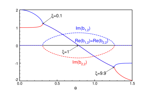
Figure 1: Exponents $b_{1}$ and $b_{2}$ as functions of $\theta$ $\left(\xi=\frac{\sin(\theta)^{2}}{\cos(\theta)^{2}}\right)$

When $0<\xi<5-2\sqrt{6}\approx 0.10$ the nonlinear parameters $b_{j,2}$ are real and positive. The CMX converges towards the ground–state energy and $E^{(2)}(t)$ exhibits the correct behaviour. When $5-2\sqrt{6}<\xi<1$ those nonlinear parameters are complex conjugate each other $b_{1,2}=b_{2,2}^{*}$ with ${\mathrm{R}e}(b_{1,2})>0$. In this case the CMX still converges towards $E_{0}$ and $E^{(2)}(t)$ is an almost reasonable approximation to $E(t)$: it exhibits a minimum at some $t>0$ and tends to a limit close to $E_{0}$ as $t\rightarrow\infty$. When $1<\xi<5+2\sqrt{6}\approx 9.90$ the nonlinear parameters are still complex conjugate each other $b_{1,2}=b_{2,2}^{*}$ but ${\mathrm{R}e}(b_{1,2})<0$. In this case the CMX converges towards the excited–state energy and $E^{(2)}(t)$ exhibits a minimum at some $t<0$ and tends to a limit close to $E_{1}$ as $t\rightarrow-\infty$. Finally, when $\xi>5+2\sqrt{6}$ the nonlinear parameters $b_{j,2}$ are real and negative. The CMX converges towards $E_{1}$ and $E^{(2)}(t)$ tends to a limit close to $E_{1}$ as $t\rightarrow-\infty$. This discussion is illustrated in Fig. 1 that shows the real and imaginary parts of $b_{j,2}$ as functions of $\theta,$ where $\xi=\frac{\sin(\theta)^{2}}{\cos(\theta)^{2}}$, $0<\theta<\pi/2$, that is a more convenient variable for plotting the exponential parameters.

As a further illustration of the discussion above in what follows we show the approximate function $E^{(2)}(t)$ in the four regions already indicated. For example, for $\xi=0.1$

$$E^{(2)}(t)=\frac{1002}{1001}+\frac{50}{143}e^{\frac{-13t}{11}}-\frac{20}{77}e^{\frac{-14t}{11}}$$

is a monotonous decreasing function that leads to a limit close to $E_{0}=1$ when $t\rightarrow\infty$. When $\xi=0.5$

$$E^{(2)}(t)=\frac{10}{9}+\left[\frac{2}{9}\cos{\left(\frac{\sqrt{15}t}{6}\right)}-\frac{2\sqrt{15}}{45}\sin{\left(\frac{\sqrt{15}t}{6}\right)}\right]e^{\frac{-t}{2}}$$

leads to $10/9\approx 1$ as $t\rightarrow\infty$ but it exhibits a minimum at $t\approx 2.8$. When $\xi=1$

$$E^{(2)}(t)=\frac{3}{2}-\frac{\sqrt{2}\sin{\left(\frac{\sqrt{2}t}{2}\right)}}{4}$$ (20)

oscillates and does not tend to any limit. The CMX approximants $A_{0,M}$ oscillate yielding either $3/2$ or $\pm\infty$ when $M$ is even or odd, respectively. When $\xi=2$ the approximate generating function

$$E^{(2)}(t)=\frac{17}{9}-\left[\frac{2}{9}\cos{\left(\frac{\sqrt{15}t}{6}\right)}+\frac{2\sqrt{15}}{45}\sin{\left(\frac{\sqrt{15}t}{6}\right)}\right]e^{\frac{t}{2}}$$

is unsuitable for $t>0$ and approaches the excited state as it tends to $17/9\approx 2$ as $t\rightarrow-\infty$. Finally, when $\xi=11$

$$E^{(2)}(t)=\frac{2663}{1332}+\left(\frac{143\sqrt{3}}{2664}-\frac{55}{1332}\right)e^{t\left(\frac{\sqrt{3}}{12}+\frac{5}{4}\right)}-\left(\frac{143\sqrt{3}}{2664}+\frac{55}{1332}\right)e^{t\left(\frac{5}{4}-\frac{\sqrt{3}}{12}\right)}$$

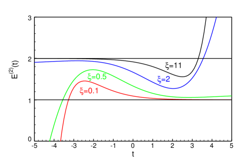
Figure 2: Approximate generating functions $E^{(2)}$ for four values of $\xi$

approaches the excited state as $t\rightarrow\infty$ as it tends to $2663/1332\approx 2$. Fig. 2 illustrates the behaviours of those functions.

Table 1 clearly shows that when $\xi=4$ $A_{0,M}$ already converges towards $E_{1}=2$ as $M$ increases as discussed above. We conclude that when $\xi>1$ the approximate functions $E^{(M)}(t)$ obtained by matching the Taylor series about $t=0$ cannot exhibit the correct exponential behaviour for $t\rightarrow\infty$. It is not difficult to understand what happens when $\xi>1$ in the case of the two–level model. First of all note that $\lim_{t\rightarrow-\infty}E(t)=E_{1}$. Second, the exponential expansion of the cumulant–generating function (13)

$$E(t)=E_{1}-\Delta Eu^{-1}\sum_{j=0}^{\infty}(-1)^{j}u^{-j}$$ (21)

converges for all $t\leq 0$ when $\xi>1$. Third, the match between the exponential expansion (12) and the $t-$expansion at $t=0$ is valid for both, positive and negative, values of $t$. Therefore, when $|c_{1}|>|c_{0}|$ the CMX simply chooses the convergent exponential expansion for $t<0$ and the result is the energy of the excited state.

The CMX fails completely when $\xi=1$ because both exponential expansions ($t>0$ and $t<0$) are divergent at $t=0$. It is worth noting that the original approach of Horn an Weinstein[1] in terms of Padé approximants $[M/M](t)$ for $E(t)$ yields accurate results in this most unfavourable case. These approximants exhibit either a saddle point or a minimum when $M$ is either odd or even, respectively. From such stationary points we obtain $E_{0}=0.9993674107,1.000359205,0.9999637967,1.000025380$ with $M=5,6,7,8$, respectively. In addition to it, these Padé approximants yield increasingly accurate estimates of the poles of $E(t)$ at $t_{s}=\pm(2j+1)\pi i$, $j=0,1,\ldots$.

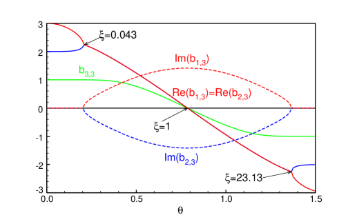
Figure 3: Exponents $b_{j,3}$ as functions of $\theta$ $\left(\xi=\frac{\sin(\theta)^{2}}{\cos(\theta)^{2}}\right)$

The behaviour of the exponential parameters discussed above is not restricted to the case $M=2$. Fig. 3 shows that two of the exponential parameters $b_{j,3}$ behave in a similar way. The third one, which we arbitrarily chose to be $b_{3,3}$, is real because the three parameters are solutions to a cubic equation. In fact, the exponential parameters $b_{j,M}$ are in general the $M$ roots of the pseudo secular determinant

$$\left|I_{i+j+1}-bI_{i+j}\right|_{i,j=1}^{M}=0$$ (22)

Fig. 4 shows $A_{0,M}(\theta)$ for some values of $M$. We appreciate that the series of CMX approximants converges towards $E_{0}=1$ when $\theta<\pi/4$ and towards $E_{1}=2$ when $\theta>\pi/4$ and diverges when $\theta$ is close to $\pi/4$ ($\xi=1$). It is a further illustration and confirmation of the arguments above.

These examples clearly show that the condition $c_{0}\neq 0$ is insufficient to guarantee the validity of equation (5) that is the main assumption of the CMX. In fact, they suggest that if $|c_{0}|\neq 0$ is not the largest overlap, then the CMX series may converge towards an excited state in which case $E^{(M)}(t)$ will not be an acceptable approximation to $E(t)$ for $t>0$, except for sufficiently small values of $t$. Besides, for some reference states (like those with $\xi=1$ for the two–level model) the CMX does not converge at all.

It is not difficult to show that the results for the two–level model also apply to arbitrary problems. For example, if we choose the reference state

$$\left|\varphi\right\rangle=c_{0}\left|\psi_{0}\right\rangle+c_{j}\left|\psi_{j}\right\rangle$$ (23)

then we draw conclusions similar to those above for $\xi=|c_{j}|^{2}/|c_{0}|^{2}$ because we already have a two–level problem.

We have also carried out a numerical and analytical study of the CMX for Hamiltonian matrices of greater dimension. For example, if we choose a diagonal matrix with elements $H_{ij}=j\delta_{ij}$, $i,j=0,1,\ldots,9$ and the reference vector with coefficients $c_{j}=(1+\delta_{j0})/\sqrt{13}$, $j=0,1,\ldots,9$ then the generating function $E(t)$ is a ratio of polynomial functions of $u=e^{-t}$. The $u$–power series (large–$t$ expansion) converges for all $|u|<1.074531738$ that is quite close to unity. For this reason we expect some difficulties when matching the $t$– and $u$–series. In fact, in this case the CMX series does not appear to converge towards the ground–state energy (or the convergence rate is too small for practical purposes).

4 Oscillators

The conclusions of the preceding section are not restricted to the particular case in which only a finite number of states contribute to $E(t)$. In what follows we consider quantum–mechanical systems with an infinite number of bound states. In order to keep present discussion as simple as possible in what follows we consider the harmonic oscillator

$$\hat{H}=-\frac{d^{2}}{dx^{2}}+x^{2}$$ (24)

If we choose

$$\left|\varphi\right\rangle=N\exp\left(-2x^{2}/5\right)$$ (25)

where $N$ is a normalization factor, then the CMX converges towards the ground state because $|c_{0}|>|c_{j}|$ for all $j$. In this case the exponential parameters for the case $M=3$ are $b_{1,3}\approx 4$, $b_{2,3}\approx 8$ and $b_{3,3}\approx 12.6$ that are quite close to the actual excitations $\Delta E_{j}=E_{2j}-E_{0}$ as expected.

If, on the other hand, we choose

$$\left|\varphi\right\rangle=N\left(x^{2}-\frac{1}{2}\right)\exp\left(-2x^{2}/5\right)$$ (26)

then the CMX converges towards the second excited state because $|c_{2}|>|c_{j}|$. Note that in this case $\left\langle\psi_{0}\right.\left|\varphi\right\rangle\neq 0$ and $\lim_{t\rightarrow\infty}E(t)=1$ ; consequently $E^{(M)}(t)$ will not be an acceptable approximation to $E(t)$ beyond a sufficiently small neighbourhood of $t=0$. This conclusion is consistent with the exponential parameters $b_{1,3}\approx-3.87$, $b_{2,3}\approx 4$ and $b_{3,3}\approx 9.29$.

If we choose

$$\left|\varphi\right\rangle=\frac{1}{\sqrt{2}}\left(\left|\psi_{0}\right\rangle+\left|\psi_{2}\right\rangle\right)$$ (27)

then the CMX series $A_{0,M}$ alternate between $\pm\infty$ and $3$ for $M$ odd and even, respectively. This result is not surprising in the light of our previous discussion of two–level models. At first sight one may think that it suggests that the CMX fails when two overlaps are equal $|c_{i}|=|c_{j}|$ and greater than any other $|c_{k}|$; however, this is not the case. For example, the reference function

$$\left|\varphi\right\rangle=\frac{\sqrt{\frac{1040\sqrt{2}}{4217}-\frac{64}{4217}}}{\pi^{\frac{1}{4}}}e^{-x^{2}}\left(x^{2}\left(3\sqrt{2}+1\right)-\sqrt{2}+1\right)$$ (28)

satisfies $c_{0}=c_{2}=\sqrt{\frac{33280\sqrt{2}}{113859}-\frac{2048}{113859}}$ but the CMX converges towards the ground state. In this case we obtain $b_{1,3}=b_{2,3}^{*}\approx 8.53+1.76i$ and $b_{3,3}\approx 4.06.$

As a nontrivial example we choose the anharmonic oscillator

$$-\frac{d^{2}}{dx^{2}}+x^{4}$$ (29)

and the reference states

$$\left|\varphi\right\rangle_{g} = N\exp\left(-3x^{2}/2\right)$$

$$\left|\varphi\right\rangle_{e} = N\left(x^{2}-\frac{1}{4}\right)\exp\left(-3x^{2}/2\right)$$ (30)

The CMX series converges towards the ground–state energy in the former case ($b_{1,3}\approx 6.34$, $b_{2,3}\approx 17.19$, $b_{3,3}\approx 34.42$) and oscillates around the second excited–state energy in the latter one ($b_{1,3}\approx-2.61$, $b_{2,3}\approx 9.04$, $b_{3,3}\approx 26.1$) as shown in Table 2. One expects that $|c_{0g}|>|c_{jg}|$ for all $j>0$ and that $|c_{2e}|>|c_{je}|$ for all $j\neq 2$. What we know for sure is that $E^{(M)}(t)$ will not be an acceptable approximation to $E(t)$ when $\left|\varphi\right\rangle=\left|\varphi\right\rangle_{e}$ except in a neighbourhood of $t=0$ as indicated by the exponential parameters $b_{j,3}$.

5 Conclusions

The main assumption of the CMX is that the exponential expansion (5) is a suitable approximation to the cumulant–generating function (2) when $|c_{0}|\neq 0$. Up to now, it was believed that the only limitations of the method were singularities in the CMX approximants (6) or an occasional divergence for some reference state. By means of simple quantum–mechanical models we have shown that the performance of the CMX is mainly determined by the overlaps $|c_{j}|$. Present investigation strongly suggests that the series of the CMX approximants (6) converges towards the energy of the state with greatest overlap with the reference function. Thus, we have the following situations:

• When $|c_{0}|>|c_{j}|$ for all $j>0$ the series $A_{0,M}$ converges towards the ground–state energy and we can say that the CMX is valid.

• The series $A_{0,M}$ converges towards the energy of an excited state (or oscillates about it). In such a case we may say that the CMX is still useful but its main assumption embodied in equation (5) is no longer valid. This situation may happen when the reference state exhibits the largest overlap with an excited state.

• The series $A_{0,M}$ does not converge at all and the CMX is of no practical utility.

In no case does the CMX converge to a meaningless limit as suggested by Knowles[5] based on results for a two–level model. The main conclusions of this paper agree with those drawn earlier that the CMX and its variants should be applied with extreme care in order to obtain useful results[5, 6, 7, 8, 9, 10, 24, 11]. In fact, in most cases the Rayleigh–Ritz variational method in the Krylov space is by far preferable to the CMX and its variants[24, 11]. We have also shown that the original method of Horn and Weinstein[1] yields accurate results in a case in which the CMX badly fails. The choice of an appropriate trial state may improve the results dramatically as illustrated by a recent study on the Rabi Hamiltonian[30].

Finally, one of the main contributions of this paper is that the analysis of the exponential parameters $b_{j,M}$ may provide an indication on the rate of convergence of the CMX approximants. If all such parameters are real and positive one expects a reasonable convergence towards the ground state (provided that $c_{0}\neq 0$). This analysis is greatly facilitated by the fact that those exponential parameters are the roots of the relatively simple pseudo secular equation (22).

Table 1: Convergence of the CMX towards the ground–state energy (second column) and excited–state energy (third column) of the two–level model ( 17) for $\xi=1/4$ and $\xi=4$, respectively.

$M$	$A_{0,M}$	$A_{0,M}$
2	1.015384615	1.984615384
4	1.000975609	1.99902439
6	1.000061031	1.999938968
8	1.000003814	1.999996185
10	1.000000238	1.999999761
12	1.000000000	2.000000000

Table 2: Convergence of the CMX towards the ground–state $(g)$ and second–excited state $(e)$ energies of the anharmonic oscillator (29)

$M$	$A_{0,M}(g)$	$A_{0,M}(e)$
5	1.060692159	7.439371257
10	1.060363186	7.456069907
15	1.060362073	7.450017954
20	1.060362093	7.451366303
25	1.060362090	7.455118704
30	1.060362090	7.454183973
35	”	7.451642486
40	”	7.454364274
50	”	7.454214745
60	”	7.453864737
70	”	7.455066766
80	”	7.455185890
90	”	7.453941990
100	”	7.453833053
RPM[36, 35]	1.060362090	7.455697938

Figure 4: Approximants $A_{0,M}$ with $M=2$ (line), $M=3$ (squares), $M=4$ (filled squares), $M=5$ (circles) and $M=6$ (filled circles) as a function of $\theta$

References

- [1] Horn D and Weinstein M 1984 Phys. Rev. D 30 1256.
- [2] Horn D, Karliner M, and Weinstein M 1985 Phys. Rev. D 31 2589.
- [3] Stubbins C 1988 Phys. Rev. D 38 1942.
- [4] Cioslowski J 1987 Phys. Rev. Lett. 58 83.
- [5] Knowles P 1987 Chem. Phys. Lett. 134 512.
- [6] Mancini J D, Prie J D, and Massano W J 1991 Phys. Rev. A 43 1777.
- [7] Lee K C and Lo C F 1993 Nuovo Cim. D 15 1483.
- [8] Mancini J D, Zhou Y, and Meier P F 1994 Int. J. Quantum Chem. 50 101.
- [9] Mancini J D, Zhou Y, Meier P F, Massano W J, and D. P J 1994 Phys. Lett. A 185 435.
- [10] Ullah N 1995 Phys. Rev. A 51 1808.
- [11] Amore P, Fernández F M, and Rodriguez M, High-order connected moments expansion for the Rabi Hamiltonian, arXiv:1010.5773v1 [quant-ph]
- [12] Mancini J D, Fessatidis V, and Bowen S P 1999 Phys. Lett. A 259 280.
- [13] Fessatidis V, Mancini J D, and Bowen S P 2002 Phys. Lett. A 297 100.
- [14] Mancini J D, Murawski R K, Fessatidis V, and Bowen S P 2005 Phys. Rev. B 72 214405 (6 pp.).
- [15] Fessatidis V, Mancini J D, Murawski R, and Bowen S P 2006 Phys. Lett. A 349 320.
- [16] Fessatidis V, Mancini J D, Bowen S P, and Campuzano M 2008 J. Math. Chem. 44 20.
- [17] Fessatidis V, Corvino F A, Mancini J D, Murawski R K, and Mikalopas J 2010 Phys. Lett. A 374 2890.
- [18] Cioslowski J 1987 Phys. Rev. A 36 374.
- [19] Cioslowski J 1987 Int. J. Quantum Chem. S 21 563.
- [20] Cioslowski J 1987 Phys. Rev. A 36 3441.
- [21] Cioslowski J 1987 Chem. Phys. Lett. 136 515.
- [22] Lo C F and Wong Y J 1994 Phys. Lett. A 187 269.
- [23] Fernández F M 2009 Int. J. Quantum Chem. 109 717.
- [24] Amore P and Fernández F M 2009 Phys. Scr. 80 055002 (5pp).
- [25] Massano W J, Bowen S P, and Mancini J D 1989 Phys. Rev. A 39 4301.
- [26] Mancini J D and Massano W J 1991 Phys. Lett. A 160 457.
- [27] Cioslowski J, Kertesz M, Surján P R, and Poirier R A 1987 Chem. Phys. Lett. 138 516.
- [28] Yoshida T and Iguchi K 1988 Chem. Phys. Lett. 143 329.
- [29] Noga J, Szabados A, and Surján P R 2002 Int. J. Mol. Sci. 3 508.
- [30] Travěnec I and Šamaj L, Optimized t-expansion method for the Rabi Hamiltonian, arXiv:1107.4479v1 [quant-ph]
- [31] Kubo R 1962 J. Phys. Soc. Jap. 17 1100.
- [32] Samaj L, Kalinay P, Markoš P, and Travěnec I 1997 J. Phys. A 30 1471.
- [33] Witte N S 1997 Int. J. Mod. Phys. B 11 1503.
- [34] Witte N S and Shankar R 1999 Nucl. Phys. B 556 445.
- [35] Fernández F M, Ma Q, and Tipping R H 1989 Phys. Rev. A 40 6149.
- [36] Fernández F M, Ma Q, and Tipping R H 1989 Phys. Rev. A 39 1605.