Density of states of a graphene in the presence of strong point defects

Abstract

The density of states near zero energy in a graphene due to strong point defects with random positions are computed. Instead of focusing on density of states directly, we analyze eigenfunctions of inverse T-matrix in the unitary limit. Based on numerical simulations, we find that the squared magnitudes of eigenfunctions for the inverse T-matrix show random-walk behavior on defect positions. As a result, squared magnitudes of eigenfunctions have equal a priori probabilities, which further implies that the density of states is characterized by the well-known Thomas-Porter type distribution. The numerical findings of Thomas-Porter type distribution is further derived in the saddle-point limit of the corresponding replica field theory of inverse T-matrix. Furthermore, the influences of the Thomas-Porter distribution on magnetic and transport properties of a graphene, due to its divergence near zero energy, are also examined.

I Introduction

Recently, the isolation of single-layer grapheneGeim07 has revived much interest in studying two-dimensional (2D) Dirac fermions. One of the peculiar properties associated with 2D Dirac fermions is the unusual electronic properties in the presence of defects and disorders. In the context of cuprate superconductors, where quasi-particles are also 2D Dirac fermions, disorders have masked the d-wave nature and hindered its discovery. It was later realized that point defects may change the density of states (DOS) near the Dirac point and strong point defects may even induce quasi-localized states or magnetic moments near zero energy in d-wave superconductorsBalatsky . In the case of graphene, it is found that there is finite density of states due to weak disordersTan . For strong disorders, it was observed that ferromagnetic state can be induced by bombarding a graphite with protonsEsquinazi . The induced magnetism is further confirmed to be resulted from $\pi$-electronsOhldag . This fact, together with recent observation of ferromagnetism in disordered grapheneWang ; Ramakrishna , shows that graphene with defects could become ferromagnetic. In addition to magnetism, graphene also reveals anomalous transport properties in the presence of strong disorders, where in the presence of vacancies, instead of decreasing, the conductivity is found to increaseColeman . These observations clearly indicates that in the presence of strong disorders, 2D Dirac fermions may behave very differently from what is expected for clean or weak disordered graphene.

Experimentally, there are many possible forms of disorders in grapheneHashimoto . For large defects such as cracks, they tend to contain the so-called zig-zag edges, where localized states would appear near the edgeMou and induce magnetic behaviorHikihara . In this case, magnetic moments arise from localized states and interact via RKKY (Ruderman-Kittel-Kasuya-Yosida) interaction, which tends to make graphene antiferromagneticBrey . Hence the most possible candidates for the observed ferromagnetism in graphene are defects of small sizes or simply point defects. Here the simplest point defects are single-atom vacancies or hydrogen chemisorption defects. These kinds of defects generally create complicated disturbances in graphene and may even form ordered structuresMcCann . However, for low density of quenched defects, they can be simulated by a large potential $u$ on a lattice point without distortion of nearby lattice pointsyaz .

Theoretically, extensive studies on a single defect have been performed on d-wave superconductorsBalatsky . It is known that a zero-energy electronic state would arise near a point defect with $u\rightarrow\infty$ or a circular disk in a 2D Dirac HamiltonianDong . Furthermore, the electronic wavefunction is semi-localized with amplitude decaying as $1/r$ at large distance $r$Balatsky ; Pereira ; Dong . The semi-localized behavior is clearly revealed in the observed STM images of long-range $(\sqrt{3}\times\sqrt{3})R30^{\circ}$ superstructure in grapheneSTMAFM ; Ugeda . For finite density of defects, one expects that semi-localized electrons interact strongly and may form an impurity bandBalatsky ; mou09 . Nonetheless, conflicting results based on either perturbative or non-perturbative approaches are reportedBalatsky . The residual DOS near zero energy is predicted to be either finiteZiegler , infiniteLee ; Ting , or vanishing with different power laws in energyBalatsky . This issue remains unsolved.

While quasi-particles in both cuprate superconductors and graphenes are 2D Dirac fermions, the situation is quite different for graphene. For neutral graphene, even though excitonic effects are expected to be largeLouie , for low energies and large distances, the screened Coulomb interaction is shown be long-rangedSheehy with renormalized dielectric constant. Furthermore, the electron itself is the quasi-particle and carries a definite charge. These differences make graphene behave totally different from that of cuprate superconductors in the strong disorders. In particular, without being masked by superconductivity, direct manifestation of the impurity band is possible in graphene. Therefore, investigation on graphene with strong defects would provide an unique opportunity to clarify the issue of DOS near zero energy for 2D Dirac fermions with strong disorders. This is recently pointed out in Ref.[mou09, ]. In that paper, the wavefunction for finite density of defects is constructed. By using the wavefunction for two defects, it is shown that ferromagnetic state is favored for large distances between two defects. However, for finite density of defects, the problem of finding DOS is mapped to an equivalent problem of finding the DOS of a random matrix. One has to assume that the matrix elements are independent random numbers to demonstrate the induced ferromagnetismmou09 . While the predicted DOS (Wigner semi-circle law) appears to be consistent with results obtained by self-consistent Born approximationPeres , to confirm that the observed ferromagnetism and anomalous transport properties of graphene are consequences of the impurity band, one needs to go beyond self-consistent Born approximation and to resolve the issue of how the DOS of 2D Dirac fermions changes in strong disorder limit.

In this paper, we re-examine the density of states of a graphene due to strong point defects. In particular, we show that the inverse T-matrix for $N_{I}$ point defects can be exactly mapped to a $N_{I}\times N_{I}$ symmetric Euclidean Random Matrix in which one cannot treat the matrix elements as independent random numbers. Instead of focusing on the DOS directly, we analyze magnitudes distribution for eigenfunctions for the derived Random Matrix. Remarkably, we find that squared magnitudes of eigenfunctions show random-walk behaviors on defect positions. As a result, the distribution of squared magnitudes of eigenfunctions for the Euclidean Random Matrix follows the Porter-Thomas distribution. Further analysis shows that eigenvalues ($\lambda$) of the corresponding Euclidean Random Matrix also follow the Thomas-Porter distributionThomasPorter and the DOS near zero energy for infinite $u$ is

$$D(E)=n_{I}\sqrt{\frac{1}{8\pi\langle|\lambda|\rangle|\lambda(E)|}}e^{-\frac{|\lambda(E)|}{2\langle|\lambda|\rangle}}\left|\frac{\lambda(E)}{dE}\right|.$$ (1)

Here $n_{I}$ is the density of defects and $\langle|\lambda|\rangle$ is the average of $|\lambda|$ over defect configurations. $\lambda(E)$ is given by $\lambda(E)=-\frac{\sqrt{3}}{2\pi D^{2}}E\ln|E/D|$ with $D=3t/2$ and $t$ being the hopping amplitude of the electron. This form of the density of states is valid when $|E|\ll t$ and we found that $\langle|\lambda|\rangle\sim\sqrt{n_{I}}$ shows random-walk behavior. The resulting density of states has strong effects on magnetic and transport properties of graphene. We re-examine the effect of the long-range Coulomb interaction with renormalized dielectric constant and show that the resulted DOS supports ferromagnetism for any finite density of defects. At finite temperature, the linear extrapolation of magnetization curve indicates that $T_{c}\sim 600-700K$, in agreement with experimental observations.

This paper is organized as follows. In Sec. II, we lay down the theoretical formulation and show that the inverse T-matrix for $N_{I}$ point defects can be exactly mapped to a $N_{I}\times N_{I}$ Euclidean Random Matrix. In Sec. III, we use both analytic arguments and numerical simulations to derive the density of resonant states. In Sec. IV, we reexamine effects of the screened long-range Coulomb interaction. We show that the competition between the exchange energy and kinetic resonant energy leads to ferromagnetism for infinite on-site potentials. The magnetizations both at zero and finite temperatures are also calculated. In Sec. V, we conclude and discuss possible effects for weak impurities. Appendix A is devoted to more rigorous derivation of the Porter-Thomas distribution in the saddle-point limit.

II Theoretical Formulation

We start by setting up the framework for investigating the effects of defect. It is known that electrons in the $\pi$ band of an infinite graphene can be well described by a tight-binding Hamiltonian $H_{0}$Geim07 . As shown in Fig. 1, the lattice of graphene is bi-partite. If we label the bi-partite lattice points by A and B, $H_{0}$ consists of hopping only for nearest A and B with a hopping amplitude $t$. Hence if defects are located at $\vec{r}_{i}$ with $i=1,2,3,\cdots,N_{I}$, the wavefunction $\psi$ for an electron then satisfies

$$\left(H_{0}+u\sum^{N_{I}}_{i=1}\delta_{\vec{r},\vec{r}_{i}}\right)\psi_{E}({\vec{r}})=E\psi_{E}({\vec{r}}).$$ (2)

Here and in the following, both $\vec{r}$ and $\vec{r}_{i}$ are restricted to points on the honeycomb lattice shown in Fig. 1.

Figure 1: Honeycomb lattice of graphene. The lattice is bi-partite, labeled by A and B , with hopping amplitude between nearest A and B being $t\sim$2.7eV. The lattice constant $a=2.46\AA$ is the distance between two nearest B points.

To find the effects of defects on the electronic state, it is sufficient to calculate the Green’s function $G({\vec{r},\vec{r}^{\prime},E})$, which describes the amplitude for the electron to propagate from $\vec{r}^{\prime}$ to $\vec{r}$ and satisfies

$$\left(E-H\right)G({\vec{r},\vec{r}^{\prime},E})=\delta_{\vec{r},\vec{r}^{\prime}},$$ (3)

where $H=H_{0}+u\sum^{N_{I}}_{i=1}\delta_{\vec{r},\vec{r}_{i}}$. For clean graphene, the Green’s function will be denoted by $G^{0}({\vec{r},\vec{r}^{\prime},E})$. In the Fourier $k$ space, it is convenient to reorganize the wavefunction into $\psi_{A}$ and $\psi_{B}$ for A and B sublattices. Then $G^{0}(k)$ is the inverse of the $2\times 2$ matrix, $E+i0^{+}-H_{0}(k)$, with $H_{0}(k)$ being given by

$$H_{0}(k)=\left(\begin{array}[]{cc}0&\Delta(k)\\ \Delta^{*}(k)&0\end{array}\right),$$ (4)

where $\Delta(k)=-t[2e^{ik_{y}a2\sqrt{3}}\cos(k_{x}a/2)+e^{-ik_{y}a/\sqrt{3}}]$. More explicitly, one finds

$$G^{0}_{AA}=G^{0}_{BB}$$

$$=\frac{1}{2}\left[\frac{1}{E+i0^{+}-|\Delta(k)|}+\frac{1}{E+i0^{+}+|\Delta(k)|}\right]$$ (5)

$$G^{0}_{AB}$$

$$=\frac{\Delta(k)}{2|\Delta(k)|}\left[\frac{1}{E+i0^{+}-|\Delta(k)|}-\frac{1}{E+i0^{+}+|\Delta(k)|}\right]$$

$$G^{0}_{BA}$$

$$=\frac{\Delta^{*}(k)}{2|\Delta(k)|}\left[\frac{1}{E+i0^{+}-|\Delta(k)|}-\frac{1}{E+i0^{+}+|\Delta(k)|}\right]$$

(6)

In real space, it is more convenient to use lattice vectors $\vec{r}$ to carry indices for A and B sublattice. Therefore, $G$ is no longer a $2\times 2$ matrix and can be expressed in terms of $G^{0}$ as

$$G({\vec{r},\vec{r}^{\prime},E})=G^{0}({\vec{r},\vec{r}^{\prime},E})+u\sum^{N_{I}}_{i=1}G^{0}({\vec{r},\vec{r}_{i},E})G({\vec{r}_{i},\vec{r}^{\prime},E}).$$ (7)

Clearly, to find $G({\vec{r},\vec{r}^{\prime},E})$, one needs to find $G({\vec{r}_{i},\vec{r}^{\prime},E})$ in Eq. (7). For this purpose, one sets $\vec{r}$ to $\vec{r}_{i}$ with $i=1,2,3,\cdots,N_{I}$ in Eq. (7) and solves $G({\vec{r}_{i},\vec{r}^{\prime},E})$ in terms of $G^{0}({\vec{r}_{i},\vec{r}^{\prime}})$. If we replace the notation $G({\vec{r}_{i},\vec{r}^{\prime},E})$ by $G_{{\vec{r}_{i},\vec{r}^{\prime}}}$ with $E$ being suppressed, we obtain

$$\left(\begin{array}[]{c}G_{{\vec{r}_{1},\vec{r}^{\prime}}}\\ G_{{\vec{r}_{2},\vec{r}^{\prime}}}\\ G_{{\vec{r}_{3},\vec{r}^{\prime}}}\\ \cdot\\ \cdot\\ G_{{\vec{r}_{N_{I}},\vec{r}^{\prime}}}\end{array}\right)=1/u\left(\begin{array}[]{cccccc}1/u-G^{0}_{{\vec{r}_{1},\vec{r}_{1}}}&-G^{0}_{{\vec{r}_{1},\vec{r}_{2}}}&-G^{0}_{{\vec{r}_{1},\vec{r}_{3}}}&\cdot&\cdot&-G^{0}_{{\vec{r}_{1},\vec{r}_{N_{I}}}}\\ -G^{0}_{{\vec{r}_{2},\vec{r}_{1}}}&1/u-G^{0}_{{\vec{r}_{2},\vec{r}_{2}}}&-G^{0}_{{\vec{r}_{2},\vec{r}_{3}}}&\cdot&\cdot&-G^{0}_{{\vec{r}_{2},\vec{r}_{N_{I}}}}\\ -G^{0}_{{\vec{r}_{3},\vec{r}_{1}}}&-G^{0}_{{\vec{r}_{3},\vec{r}_{2}}}&1/u-G^{0}_{{\vec{r}_{3},\vec{r}_{3}}}&\cdot&\cdot&-G^{0}_{{\vec{r}_{3},\vec{r}_{N_{I}}}}\\ \cdot&\cdot&\cdot&\cdot&\cdot\\ \cdot&\cdot&\cdot&\cdot&\cdot\\ -G^{0}_{{\vec{r}_{N_{I}},\vec{r}_{1}}}&-G^{0}_{{\vec{r}_{N_{I}},\vec{r}_{2}}}&-G^{0}_{{\vec{r}_{N_{I}},\vec{r}_{3}}}&\cdot&\cdot&1/u-G^{0}_{{\vec{r}_{N_{I}},\vec{r}_{N_{I}}}}\end{array}\right)^{-1}\left(\begin{array}[]{c}G^{0}_{{\vec{r}_{1},\vec{r}^{\prime}}}\\ G^{0}_{{\vec{r}_{2},\vec{r}^{\prime}}}\\ G^{0}_{{\vec{r}_{3},\vec{r}^{\prime}}}\\ \cdot\\ \cdot\\ G^{0}_{{\vec{r}_{N_{I}},\vec{r}^{\prime}}}\end{array}\right).$$ (26)

Here the matrix on the right hand side is the T-matrix whose inverse determines resonant energies and can be separated into real and imaginary parts

$$T^{-1}=\left(\begin{array}[]{ccccc}1/u-\cal{G}_{\it{11}}&-\cal{G}_{\it{12}}&\cdot&\cdot&-\cal{G}_{\it{1N_{I}}}\\ -\cal{G}_{\it{21}}&1/u-\cal{G}_{\it{22}}&\cdot&\cdot&-\cal{G}_{\it{2N_{I}}}\\ -\cal{G}_{\it{31}}&-\cal{G}_{\it{32}}&\cdot&\cdot&-\cal{G}_{\it{3N_{I}}}\\ \cdot&\cdot&\cdot&\cdot&\cdot\\ \cdot&\cdot&\cdot&\cdot&\cdot\\ -\cal{G}_{\it{N_{I}1}}&-\cal{G}_{\it{N_{I}2}}&\cdot&\cdot&1/u-\cal{G}_{\it{N_{I}N_{I}}}\end{array}\right)-i\left(\begin{array}[]{ccccc}I_{11}&I_{12}&\cdot&\cdot&I_{1N_{I}}\\ I_{21}&I_{22}&\cdot&\cdot&I_{2N_{I}}\\ I_{31}&I_{32}&\cdot&\cdot&I_{3N_{I}}\\ \cdot&\cdot&\cdot&\cdot&\cdot\\ \cdot&\cdot&\cdot&\cdot&\cdot\\ I_{N_{I}1}&I_{N_{I}2}&\cdot&\cdot&I_{N_{I}N_{I}}\end{array}\right),$$ (39)

where $\cal{G}_{\it{ij}}$ and $I_{ij}$ are the real and imaginary parts of $G^{0}_{ij}$. Note that due to the Kramers-Kronig relation, $\cal{G}_{\it{ij}}$ and $I_{ij}$ are related by

$$I_{ij}(E)=\cal{P}\it{\int\frac{\cal{G}_{\it{ij}}(\it{E^{\prime}})}{E-E^{\prime}}dE^{\prime}}.$$ (40)

Therefore, real ($T^{-1}_{R}$) and imaginary parts ($T^{-1}_{I}$) of $T^{-1}$ can be diagonalized simultaneously. In particular, their eigenvalues are also related by the Kramers-Kronig relation

$$\lambda_{I}(E)=\cal{P}\it{\int\frac{\lambda_{G}(E^{\prime})}{E-E^{\prime}}dE^{\prime}}.$$ (41)

It is thus clear that the resonant energies of the Green’s function $G$ are determined by zeros of eigenvalues of $T_{R}$. Therefore, resonant energies due to defects are determined by

$$\left|\begin{array}[]{ccccc}1/u-\cal{G}_{\it{11}}&-\cal{G}_{\it{12}}&\cdot&\cdot&-\cal{G}_{\it{1N_{I}}}\\ -\cal{G}_{\it{21}}&1/u-\cal{G}_{\it{22}}&\cdot&\cdot&-\cal{G}_{\it{2N_{I}}}\\ -\cal{G}_{\it{31}}&-\cal{G}_{\it{32}}&\cdot&\cdot&-\cal{G}_{\it{3N_{I}}}\\ \cdot&\cdot&\cdot&\cdot&\cdot\\ \cdot&\cdot&\cdot&\cdot&\cdot\\ -\cal{G}_{\it{N_{I}1}}&-\cal{G}_{\it{N_{I}2}}&\cdot&\cdot&1/u-\cal{G}_{\it{N_{I}N_{I}}}\end{array}\right|=0.$$ (42)

Note that the above condition is exactly the same as the one obtained via the constructed wavefunction for defectsmou09 and should be compared to the similar equation obtained in the context of d-wave superconductorsLee . Since a graphene without defect is translationally invariant, one has $G^{0}_{ij}=G^{0}(\vec{r}_{i}-\vec{r}_{j})$. Therefore, diagonal terms in Eq.(42) are identical and are equal to $\lambda(E)\equiv 1/u-\rm{Re}\it{G^{0}}(\rm{0},\it{E})$. Hence if the positions of defects are random, solving Eq.(42) is equivalent to finding eigenvalues of the random matrix

$$H_{I}=\it{\left(\begin{array}[]{ccccc}0&\cal{G}_{\it{12}}&\cdot&\cdot&\cal{G}_{\it{1N_{I}}}\\ \cal{G}_{\it{21}}&0&\cdot&\cdot&\cal{G}_{\it{2N_{I}}}\\ \cal{G}_{\it{31}}&\cal{G}_{\it{32}}&\cdot&\cdot&\cal{G}_{\it{3N_{I}}}\\ \cdot&\cdot&\cdot&\cdot&\cdot\\ \cdot&\cdot&\cdot&\cdot&\cdot\\ \cal{G}_{\it{N_{I}1}}&\cal{G}_{\it{N_{I}2}}&\cdot&\cdot&0\end{array}\right)}.$$ (43)

Furthermore, if one defines the density of eigenvalues for $H_{I}$ by

$${\cal D}(\lambda)=\frac{1}{M}\sum_{n}\delta(\lambda-\lambda_{n}),$$ (44)

with $M$ being the total number of lattice points and $\lambda_{n}$ being the $n$-th eigenvalue, the density of resonant states is given by

$$D(E)=\cal{D}(\it{\lambda(E)})\left|\frac{d\lambda(E)}{dE}\right|.$$ (45)

Therefore, it is sufficient to find the distribution of eigenvalues for $H_{I}$. We note in passing that if values of $\lambda_{G}$ form a band after averaging over defect configurations, it implies that the averaged $\langle\lambda_{G}\rangle$ is independent of $E$. Eq.(41) then implies that except for contributions from diagonal terms $I_{nn}$, off-diagonal terms do not contribute to the imaginary part of eigenvalues. Hence if values of $\lambda$ form a band, one has $T^{-1}_{I}=-\rm{Im}\it{G^{0}}(\rm{0},\it{E})\bf{I}$. Since $\rm{Im}\it{G^{0}}(\rm{0},\it{E})\propto E$, this result implies that the inverse of lifetime for resonant states is proportional to $E$, consistent with experimental observationlifetime .

III Density of resonant states

In the last section, it is shown that the density of resonant states is determined by the spectrum of $H_{I}$. Since each element, $\cal{G}_{\it{ij}}$, depends on positions of defects, they fluctuate randomly. In the simplest approximation, one treats each element as an independent random number. The density of states is characterized by the Wigner semi-circle lawmou09 . As indicated earlier, this approximation appears to be equivalent to the self-consistent Born approximation Peres . A closer examination of $H_{I}$ shows that the dependence of each matrix element on the position $\vec{r}_{i}$ makes them correlated. Hence one cannot treat each element as an independent random number. Indeed, it was realized in different context by Mezard et al.Zee that such random matrices form distinct classes known as Euclidean Random Matrices, whose spectrum depends on the functional form of the matrix element on $\vec{r}_{i}$ .

It is generally difficult to find the exact spectrum for any given Euclidean Random Matrices. For defects on graphene, however, it turns out that the spectrum of $H_{I}$ follows a simple form known as the Porter-Thomas distributionThomasPorter . In this section, we shall focus on the study of the spectrum by numerical simulation. An analytical derivation based on saddle-point approximation will be relayed to the Appendix.

We start by noting that since one expects that the energies of resonant states are close to zero, as a first step, we can approximate each matrix element by $\cal{G}_{\it{ij}}\it(E=0)$. We shall see later that the error due to this approximation is small for $E\sim 0$. In this approximation, by using Eqs.(5) and (6), one finds ${\cal G}_{AA}(r,E=0)={\cal G}_{BB}(r,E=0)=0$ and $G_{BA}(j,i)=G^{*}_{AB}(i,j)$. Hence $H_{I}$ is a symmetric matrix. Furthermore, since in the second quantization form, $H_{I}=\sum_{ij}{\cal G}_{ij}{c^{\dagger}_{A}}_{i}{c_{B}}_{j}+h.c.$, we find that $H_{I}$ goes to $-H_{I}$ under the particle-hole transformation: ${c^{\dagger}_{A}}_{i}\rightarrow-{c_{A}}_{i}$ and ${c_{B}}_{j}\rightarrow{c^{\dagger}_{B}}_{j}$. Therefore, the spectrum is particle-hole symmetric, i.e., ${\cal D}(-\lambda)={\cal D}(\lambda)$. In addition of being particle-hole symmetric, $H_{I}$ itself also supports energy states exactly at zero energy due to the unbalance in the number of lattice points in A and BBrouwer . Since the number of zero energy states is equal to $|N_{A}-N_{B}|$, if lattice points are randomly assigned to A or B, one finds $|N_{A}-N_{B}|\sim\sqrt{N_{I}}$ and hence their contribution is negligible in the limit of $M\rightarrow\infty$ with $N_{I}/M$ being fixed at the defect density $n_{I}$. Therefore, in the following, we shall focus on density of resonant states for the case with $N_{A}=N_{B}$ to avoid complications due to extra zero energy states.

For high density of defects, because the positions of defects sample sufficient lattice points, $H_{I}$ can be diagonalized by Fourier transformation. Hence eigenvalues of $H_{I}$ are proportional to the Fourier transformation of $\cal{G}_{\it{ij}}$. We find that

$${\cal D}(\lambda)\propto\int\int\frac{d^{2}{\bf q}}{(2\pi)^{2}}\left[\delta\left(\lambda-\frac{1}{|\Delta({\bf q})|}\right)+\delta\left(\lambda+\frac{1}{|\Delta({\bf q})|}\right)\right].$$

(46)

In this case, because $0\leq|\Delta(q)|\leq 3t$, we obtain $\lambda\geq 1/3t$. Therefore, there is no resonant defect state near zero energy for sufficient high density of defects.

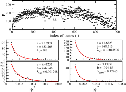
Figure 2: (Color on-line) Participation number ($p=1/\sum_{i}|\phi(\vec{r}_{i})|^{4}$) and histogram of $|\phi_{\lambda}|^{2}$ of different $\lambda$’s and $p$’s (indicated by sub-indices of $\lambda$) for a typical defect configuration simulated with $N_{I}=1000$ and $M=1000\times 1000$, i.e., $n_{I}=0.001$. Here red solid lines are the fitted Boltzmann distributions.

For low density of defects, the separation between any two defects is large. In this case, by using Eqs.(5) and (6), we find that for $0<|E|r/v\ll 1$Lee ,

$${\cal G}_{AA}(r,E)={\cal G}_{BB}(r,E)=\frac{\sqrt{3}a^{2}}{2\pi v^{2}}\cos\left(\frac{4\pi x}{3a}\right)E\ln\frac{r|E|}{v},$$

(47)

$${\cal G}_{AB}(r,E)={\cal G}_{BA}(r,E)=\frac{\sqrt{3}a}{2\pi v}\frac{1}{r/a}\sin\left(\frac{4\pi x}{3a}\right).$$ (48)

Here $v=3ta/2$. While for $E=0$, as we indicated earlier, ${\cal G}_{AA}(r,E=0)={\cal G}_{BB}(r,E=0)=0$ but ${\cal G}_{AB}(r,E=0)$ is given by Eq.(48). For $r=0$, we obtain

$${\cal G}_{AA}(0,E)={\cal G}_{BB}(0,E)=\frac{\sqrt{3}a^{2}}{2\pi v^{2}}E\ln\frac{a|E|}{v}.$$ (49)

To motivate it, instead of focusing on DOS directly as done in the d-wave superconductorsLee ; Balatsky , we analyze the distribution of the eigenfunction amplitudes $\phi_{\lambda}(\vec{r}_{i})$ of $H_{I}$ at a fixed eigenvalue $\lambda$

$$P(|\phi|^{2})=\frac{1}{M}\sum_{i}\delta(|\phi|^{2}-|\phi_{\lambda}(\vec{r}_{i})|^{2}).$$ (50)

Here $\phi_{\lambda}(\vec{r}_{i})$ is normalized so that

$$\sum_{i}|\phi_{\lambda}(\vec{r}_{i})|^{2}=1.$$ (51)

Hence if there is no bias on partitioning $|\phi|^{2}$, one expects $|\phi|^{2}$ follows the Boltzmann type distribution, $P(|\phi|^{2})\propto e^{-\alpha|\phi|^{2}}$. Indeed, in the limit $M\rightarrow\infty$, Porter and ThomasThomasPorter derived the following distribution

$$P(t)=\frac{1}{2\pi s\langle s\rangle}e^{-\frac{s}{2\langle s\rangle}},$$ (52)

where $s=|\phi|^{2}$ and $\langle s\rangle$ is the average of $|\phi|^{2}$. The same distribution can also be derived in the non-linear sigma modelEfetov1 . The Porter-Thomas distribution, however, is not universal and is valid only when the system is sufficiently chaoticMuller . Since the matrix element ${\cal G}_{ij}$ decays slowly ($1/r$), $\phi_{\lambda}$ at each point $\vec{r}_{i}$ is determined by all other defects with random positions. In other words, $H_{I}$ is a random hopping model in which $\phi_{i}$ characterizes density of random walkers on defect position $\vec{r}_{i}$. Since the probability for finding a random walker at the traveling distance $r$ is proportional to $e^{-r^{2}/2\langle r^{2}\rangle}$, by comparison with Eq.(52), one expects that the Porter-Thomas distribution works for $H_{I}$ with $\phi$ playing the role of distance. More explicitly, for a random walker described by $\vec{r}(t)$, one finds $\langle r^{2}\rangle\propto t$ at time $t$. Here $t$ characterizes the number of attempts in a random walk. By analogy, $N_{I}$ would be the number of attempts. Therefore, we expect

$$\langle|\phi|^{2}\rangle\propto\sqrt{n_{I}}.$$ (53)

Based on Eq.(48), we perform extensive numerical analysis on the statistics of eigenstates of $H_{I}$. To see if there is correlation between distribution and localization of $\phi_{\lambda}$, we also analyze the participation number $p=1/\sum_{i}|\phi(\vec{r}_{i})|^{4}$ and find the distribution for different participation numbers. Fig. 2 shows the statistics of wavefunction amplitudes for a typical defect configuration. It is clear that regardless of whether the eigenfunction is localized or not, distribution of amplitudes follow the Porter-Thomas distribution for all participation numbers.

For different $\lambda$, in addition to Eq.(51), partition of eigenfunction amplitudes $\phi$ has an addition constraint

$$\sum_{ij}\phi_{i}(H_{I})_{ij}\phi_{j}=\lambda,$$ (54)

where $(H_{I})_{ij}={\cal G}_{ij}$ for $i\neq j$ and $(H_{I})_{ii}=0$. It is clear that for different $\lambda$, $\phi\propto\sqrt{\lambda}$. Hence by replacing $\phi$ by $\sqrt{|\lambda|}$ in Eq. (52) with appropriate normalization, we expect that the distribution for $\lambda$ also follows the Porter-Thomas distribution

$${\cal D}(\lambda)=n_{I}\sqrt{\frac{1}{8\pi\langle|\lambda|\rangle|\lambda|}}e^{-\frac{|\lambda|}{2\langle|\lambda|\rangle}}.$$ (55)

Here according to Eq.(53), we expect $\langle|\lambda|\rangle\propto\sqrt{n_{I}}$. The proportional constant will be determined numerically. The normalization ${\cal D}$ in Eq.(55) is chosen by requiring $\int^{\infty}_{-\infty}d\lambda{\cal D}(\lambda)=n_{I}$. Note that for later use in the calculation of magnetization, the normalization of ${\cal D}$ has to be done by taking into account the presence of Dirac band.

Fig.3(a) shows a typical spectrum of our numerical simulations of the spectrum averaged over 1000 defect configurations. It shows that the spectrum can be well described by

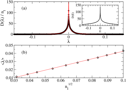
Figure 3: (Color on-line) (a) Averaged spectrum of $H_{I}$ (with ${\cal G}_{ij}(E=0)$ as the matrix element) over 1000 defect configurations. Here $n_{I}=1000$, $M=1000\times 1000$ and we have set $t=1$. Black circles are numerical results while the red line is the fitted Porter-Thomas distribution with ${\cal D}(\lambda)=2.17e^{-45.438|\lambda|}/\sqrt{|\lambda|}$. Inset: The corresponding density of electronic states for $u=\infty$. (b) Random-walk behavior of $\phi$: The dependence of $\langle\lambda\rangle$ on the defect density $\sqrt{n_{I}}$ shows linear behavior with a slope $0.464$. Here open circles are numerical results obtained by the fitted Porter-Thomas distribution while the red line is the linear curve of slope $0.464$. There is a small error offset by $-0.0038$.

the Porter-Thomas distribution. Fig.3(b) shows the fitted parameter $\langle\lambda\rangle$ versus density of defects. It indicates that $\langle\lambda\rangle$ follows a simple form of $n_{I}$ by $\langle\lambda\rangle\approx\sqrt{n_{I}}$. Once one knows the spectrum of $H_{I}$, by using Eq.(49), the density of resonant energies can be found by setting $\lambda=1/u-{\cal G}_{AA/BB}(0,E)$. This results in Eq.(1). In the inset of Fig.3(a), we show the corresponding electronic DOS for $u=\infty$. It is clear that the DOS diverges at $E=0$.

We close this section by checking the validity of setting $E=0$ in ${\cal G}_{ij}(E)$. For a given finite $E$, because $\lambda=1/u-{\cal G}(0,E)$, there is only one value of $\lambda$ corresponding to the given $E$. Hence for a given $E$, only the spectrum at $\lambda=1/u-{\cal G}(0,E)$ is correct. To get the whole spectrum, it is necessary to vary $E$ and obtain the spectrum at each $\lambda(E)$ one by one. Note that by using Eqs.(5) and (6), one finds that ${\cal G}_{ij}(-E)=-{\cal G}_{ij}(E)$ and hence the resulting spectrum is still particle-hole symmetric. In Fig.4, we show the comparison of the spectrum for $H_{I}$ by using ${\cal G}_{ij}(E)$ and ${\cal G}_{ij}(E=0)$. It is clear that the difference is small and both spectra follow the Porter-Thomas distribution, in agreement with the derivation in the Appendix that is based on saddle-point approximation.

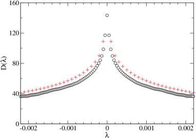
Figure 4: (Color on-line) Comparison of the spectrum of $H_{I}$ determined by using ${\cal G}_{ij}(E)$ (open circles) and ${\cal G}_{ij}(E=0)$ (red crosses) as matrix elements. Here $n_{I}=1000$, $M=1000\times 1000$ and we have set $t=1$. Both spectra can be fitted with the Porter-Thomas distributions with slightly different $\langle|\lambda|\rangle$.

IV Effects of Coulomb interaction and ferromagnetism

In this section, we discuss effects of the Coulomb interaction due to the change of density of states. To include the effects of Coulomb interaction, we note that for neutral graphene, even though excitonic effects are expected to be largeLouie , for low energies and long distances, screening can be taken into consideration by the renormalization of $v$ and the dielectric constant $\epsilon$Sheehy . Hence for low density of defects in which separation between any two defects is large, one needs to replace $v$ by $v_{R}$ in Eqs. (47) and (48). This would effectively replace the hopping amplitude $t$ by $t_{R}$.

As indicated in the introduction, strong disorders in a graphene are a possible source for the observed ferromagnetism. To examine whether the Porter-Thomas type distribution supports ferromagnetism, we first note that the normalization adopted in Eq.(55) has to be corrected by taking into account the conservation of states. As indicated in Fig.5, since resonant states replaces states in Dirac band, it requires a cutoff $\Lambda$ in the impurity band so that numbers of states for the impurity band and the Dirac band are

Figure 5: Schematic plot of the impurity band and the original Dirac band. Here the solid lines at center represent the impurity band when $u=\infty$. For a small finite $u$, the impurity band (represented by the dash line) is shifted into the Dirac band and disappears

equal. Since number of states for the impurity band per site is $n_{I}$, integration of the Dirac band yields $\Lambda=\sqrt{\pi/4}v_{R}n_{I}$. By including the cutoff $\Lambda$, appropriate normalized ${\cal D}_{\Lambda}$ is given by

$${\cal D}_{\Lambda}(\lambda)=\frac{n_{I}}{\sqrt{8\pi\langle|\lambda|\rangle}{\rm erf}(\sqrt{\lambda_{\Lambda}/2\langle|\lambda|\rangle})}e^{-\frac{|\lambda|}{2\langle|\lambda|\rangle}}.$$ (56)

Here erf is the error function and $\lambda_{\Lambda}=\lambda(\Lambda)$. Note that when $v$ is renormalized to $v_{R}$, both $\langle|\lambda|\rangle$ and $\lambda_{\Lambda}$ are renormalized by the same factor $v_{R}/v$.

To investigate the magnetism, we note that the electron wavefunction $\psi_{E}$ is related to the eigenfunction $\phi$ of $H_{I}$ as followsmou09

$$\psi_{E}(\vec{r}_{i})=\sum_{j={\rm defect\hskip 1.0ptpositions}}{\cal G}_{ij}A^{j}_{E}.$$ (57)

Here $A^{j}_{E}$ is proportional to $\phi_{j}$. The normalization of $A^{j}_{E}$ is determined by $\langle\sum_{i}\psi^{2}_{E}(\vec{r}_{i})\rangle=1$. The applicability of the Porter-Thomas distribution implies that $\phi_{j}$ (thus $A^{j}_{E}$) follows Gaussian statisticsThomasPorter . Hence we have

$$\langle A^{i}_{E}A^{j}_{E}\rangle=\Gamma\delta_{ij}.$$ (58)

By expressing ${\cal G}_{ij}=\frac{1}{M/2}\sum_{\vec{q}}{\cal G}(\vec{q})e^{i\vec{q}\cdot(\vec{r}_{i}-\vec{r}_{j})}$ and using the fact that ${\cal G}_{AA}(r,E=0)={\cal G}_{BB}(r,E=0)=0$, we find $\Gamma=1/(N_{I}\gamma)$ with

$$\gamma=\frac{1}{M/2}\sum_{\vec{q}}{\cal G}_{AB}(\vec{q}){\cal G}_{AB}(-\vec{q}).$$ (59)

We shall include the Coulomb interaction by calculating the exchange energy. For a neutral graphene, it is known that screened Coulomb interaction is still long-rangedSheehy ; Geim07

$$H_{C}=\frac{e^{2}}{8\pi\epsilon}\sum\limits_{i,j,\sigma,\sigma^{\prime}}C^{\dagger}_{i\sigma}C_{i\sigma}\frac{1}{|\vec{r}_{i}-\vec{r}_{j}|}C^{\dagger}_{j\sigma^{\prime}}C_{j\sigma^{\prime}},$$ (60)

where $\epsilon$ is the renormalized dielectric constant and is roughly $2.3\epsilon_{0}$. To obtain the exchange energy, Eq.(57) is replaced by $C^{\dagger}_{i\sigma}=\sum_{E,j}A^{j}_{E}{\cal G}_{ij}(E)C^{\dagger}_{E\sigma}$. By setting any pair of $C^{\dagger}_{E\sigma}C_{E^{\prime}\sigma^{\prime}}$ by its average value $\langle C^{\dagger}_{E\sigma}C_{E^{\prime}\sigma^{\prime}}\rangle$, using the fact $\langle A^{i}_{E_{1}}A^{j}_{E_{2}}A^{k}_{E_{2}}A^{l}_{E_{1}}\rangle=\langle A^{i}_{E_{1}}A^{l}_{E_{1}}\rangle\langle A^{j}_{E_{2}}A^{k}_{E_{2}}\rangle$ and approximating ${\cal G}_{ij}(E)$ by ${\cal G}_{ij}(0)$, we find that the exchange energy is given by

$$E_{ex}=-\frac{e^{2}(n^{2}_{\uparrow}+n^{2}_{\downarrow})}{8\pi\epsilon\gamma^{2}}B$$ (61)

with

$$B=\sum\limits_{i,j}\frac{1}{|\vec{r}_{i}-\vec{r}_{j}|}\left(\sum\limits^{N_{I}}_{k=1}{\cal G}_{ik}{\cal G}_{jk}\right)^{2},$$ (62)

where $n_{\sigma}=N_{\sigma}/N_{I}$ are fractions of electrons in the spin state $\sigma$. By approximating ${\cal G}_{ij}(E)$ by ${\cal G}_{ij}(0)$ and expressing ${\cal G}_{ij}$ in Fourier space, we find

$$\frac{B}{M}=\frac{16\pi n^{2}_{I}}{\sqrt{3}a^{2}M^{2}}\times$$

$$\sum_{q,q^{\prime}}\frac{1}{|\vec{q}+\vec{q}^{\prime}|}{\cal G}_{AB}(\vec{q}){\cal G}_{AB}(-\vec{q}){\cal G}_{AB}(\vec{q}^{\prime}){\cal G}_{AB}(-\vec{q}^{\prime})$$ (63)

where only the $i$ and $j$ in the same sublattice would contribute. Since for $E\sim 0$, Eq.(6) implies ${\cal G}_{AB}$ diverges near Dirac points $\vec{q}_{D}$. The main contribution in the integral of $B$ comes from regions of $\vec{q}_{D}$. By setting $\vec{q}$ to any one of the Dirac points in the factor $1/|\vec{q}+\vec{q}^{\prime}|$, we find

$$\frac{B}{M}=\frac{2+\sqrt{3}}{4a}n^{2}_{I}\gamma^{2}.$$ (64)

In the ferromagnetic state, we have $n_{\uparrow}\neq n_{\downarrow}$ with $E_{\sigma}$ being the corresponding Fermi energy for the spin state $\sigma$. The net spin moment is proportional to $m\equiv n_{\uparrow}-n_{\downarrow}$. Substituting Eq.(64) back to $E_{ex}$, we find that the exchange energy per site due to $m$ is given by

$$\frac{E_{ex}}{M}=-\frac{e^{2}m^{2}}{16\pi\epsilon}\frac{2+\sqrt{3}}{4a}n^{2}_{I}.$$ (65)

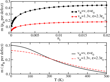
Figure 6: (Color on-line) Magnetization per defect for $u=\infty$ with screened ($\epsilon=2.3\epsilon_{0}$, $v_{R}=1.3v$) and unscreened ($\epsilon=\epsilon_{0}$, $v_{R}=v$) Coulomb interactions. (a) Magnetization versus defect density at zero temperature (b) A typical temperature dependence of magnetization for $n_{I}=O(10^{-3})$. There is no sharp transition temperature. However, by linear extrapolation, one finds that $T_{c}$ is around $600-700K$.

For an undoped graphene, $E_{\downarrow}=-E_{\uparrow}$. In this case, the net spin $m$ can be expressed as $m=2\int^{E_{\uparrow}}_{0}dED_{\Lambda}(E)$, while the change of the total energy in the impurity band per site is $\Delta k=2\int^{E_{\uparrow}}_{0}dEED_{\Lambda}(E)$. The minimization of $\Delta k+E_{ex}/M$ with respect to $E^{\uparrow}$ then leads to

$$\frac{(2+\sqrt{3})e^{2}n_{I}}{16\pi\epsilon a}\int^{\lambda({E_{\uparrow})}}_{0}{\cal D}_{\Lambda}(\lambda)d\lambda=E_{\uparrow}.$$ (66)

Solving Eq.(66) yields $E_{\uparrow}$ which in turn determines the magnetization per defect at zero temperature. The same calculation can be easily generalized to any finite temperature $T$. In this case, the magnetization is still determined by the minimization of $\Delta k+E_{ex}/M$ with respect to $E^{\uparrow}$ except that now $m$ and $\Delta k$ are replaced by

$$m=\int^{\infty}_{-\infty}dED_{\Lambda}(E)\left[n_{\uparrow}(E)-n_{\downarrow}(E)\right],$$ (67)

$$\Delta k=\int^{\infty}_{-\infty}dED_{\Lambda}(E)\left[n_{\uparrow}(E)+n_{\downarrow}(E)-2n_{0}(E)\right],$$ (68)

where $n_{\sigma}(E)=1/(e^{\beta(E+E_{\sigma})}+1)$ are the Fermi-Dirac distributions for $\sigma=\uparrow$ or $\downarrow$ and $n_{0}(E)=1/(e^{\beta E}+1)$ with $\beta=1/k_{B}T$.

In Fig.6(a), we show the magnetization at zero temperature for $u=\infty$ with screened and unscreened Coulomb interaction by solving Eq.(66). It is seen that screening reduces the magnetization. Furthermore, due to the divergent DOS at $E=0$, ferromagnetism persists down to zero defect density and magnetization increases as defect density increases. Fig.6(b) shows a typical temperature dependence of magnetization for $n_{I}=O(10^{-3})$. The temperature dependence shows a quasi-linear behavior with a Boltzman tail. To compare with experiments, we perform the linear extrapolation of magnetization curve, which indicates that $T_{c}\sim 600-700K$, in agreement with experimental observationsBarzola .

V Summary and discussion

In summary, in this work we have shown that in the strong disorder limit, a resonant impurity band is induced in a graphene. By combining analytic arguments and numerical calculations, we show that the density of resonant states is governed by the principle of equal a priori probabilities for squared magnitudes of eigenfunctions of a Euclidean Random Matrix. For large on-site defect potential, the principle of equal a priori probabilities shows that the density of resonant states is characterized by the Thomas-Porter distribution and is divergent near zero energy. Furthermore, we show that the observed ferromagnetism is due to the combination of strong disorder and long-range Coulomb interaction. The linear extrapolation of magnetization curve indicates that $T_{c}\sim 600-700K$, as observed in experiments.

In addition to the magnetism, the impurity band enhances the transportmou09 . This is consistent with experimental observationsColeman but is quite different from ordinary impurity states even though in the calculated participation number of $H_{I}$ in Fig.2, some eigenfunctions $\phi$ are localized. The crucial difference lies in the semi-localized nature of the electronic states as revealed in Eq.(57). Here even though $A^{j}_{E}$ (thus $\phi^{j}$) is localized, due to that ${\cal G}\sim 1/r$, $\psi_{E}$ will not be exponentially localized around defect positions. The participation number for $\psi_{E}$ itself is of the order of $(\ln M)^{2}$, indicating its semi-localized nature.

While so far in this work we only consider the strong disorder limit, the results also provide some insight into the weak disorder region. As illustrated in Fig.5, for weak disorders, $u$ is small, the impurity band is shifted into the Dirac band. In this case, while the majority weight of the impurity band disappears, its tail still sweeps through zero energy and contributes small but finite DOS. As indicated above, these density of states generally enhances the transport. This explains why when graphene is made cleaner, the conductivity, instead of increasing, decreases and appears to approach an universal constantGeim07 . While the impurity band cannot account for the exact value of the universal conductivity, our results serve as a useful starting point for obtaining corrections to the conductivity.

Appendix A Saddle-point limit and Porter-Thomas distribution

In this appendix, we shall show that the eigenvalue distribution for $H_{I}$ follows the Porter-Thomas distribution in the limit of $N_{I}\rightarrow\infty$ but with the defect density $n_{I}$ being fixed. We start by noting that the spectrum of $H_{I}$ can be found by calculating the resolvent

$$R(z)=\langle\frac{1}{M}Tr\frac{1}{z-H_{I}}\rangle,$$ (69)

where $M$ is the total number of lattice points and $\langle\cdot\rangle$ is the average over the random configurations of defects. Clearly, we have $\cal{D}\it{(\lambda)=-\frac{1}{\pi}{\rm Im}R(\lambda+i0^{+})}$. As shown in the text, since the spectrum has particle-hole symmetry, we shall set $\lambda$ to $|\lambda|$ and consider only positive $\lambda$. The evaluation of $R(z)$ can be reformulated by a replica field theoryZee via the following identity

$$R(z) = \lim_{n\rightarrow 0}\frac{-1}{nM}\frac{\partial}{\partial z}\langle e^{-nTr\log(z-H_{I})}\rangle$$ (70)

$$= \lim_{n\rightarrow 0}\frac{-1}{nM}\frac{\partial}{\partial z}\left\langle\frac{1}{\det(z-H_{I})^{n}}\right\rangle.$$

The term $1/\det(z-H_{I})^{n}$ can be re-expressed by $n$ replica complex fields $\phi_{a}$ ($a$=1,2,3,..,$n$) as follows

$$\left\langle\frac{1}{\det(z-H_{I})^{n}}\right\rangle=\left\langle\int\prod\limits^{N_{I}}_{i=1}\prod\limits^{n}_{a=1}{\cal D}\phi e^{-\sum_{ij}{\phi^{a}_{i}}^{*}(H_{I})_{ij}\phi^{a}_{j}}\right\rangle.$$

(71)

Up to now $\phi_{a}$ is only defined on defect sites. To remove this constraint, one introduces the field $\hat{\psi}_{a}$ defined on every lattice site and impose $\delta[\hat{\psi}_{a}(\vec{r})-\sum_{i}\phi^{a}_{i}\delta_{\vec{r},\vec{r}_{i}}]$. The constraint of the delta function can be removed by using the identity $\delta(F)=\int d\psi_{a}e^{i\psi_{a}F}$. Here $\psi_{a}$ is the replica field. After integrating out $\phi^{a}_{i}$ and $\hat{\psi}_{a}$, the resolvent can be expressed asZee

$$R(z)=-\lim_{n\rightarrow 0}\frac{1}{nM}\frac{\partial\log Z}{\partial z},$$ (72)

where the partition function $Z$ is given by $Z=\int{\cal D}\psi e^{-S}$ with $S$ being given by

$$S=-\sum^{n}_{a=1}\sum_{i,j}\psi^{*}_{a}(\vec{r}_{i})F_{ij}\psi_{a}(\vec{r}_{j})-n_{I}\sum_{i}e^{-\frac{1}{z}\sum_{a}|\psi_{a}(\vec{r}_{i})|^{2}}.$$ (73)

Here $F_{ij}={\cal G}^{-1}_{ij}-\delta_{ij}{\cal G}^{-1}_{ii}$. Note that because $G^{0}=1/(E-H)$, we have that for $E\sim 0$, $F_{ij}=-(H_{0})_{ij}$. In other words, $-F$ has the same form as the tight-binding Hamiltonian for graphene except that it only acts on defect sites.

After substituting $Z$ back to $R$, we find

$$R(z)=-\lim_{n\rightarrow 0}\frac{n_{I}}{nM}\frac{\int{\cal D}\psi\frac{1}{z^{2}}\sum_{a,i}|\psi_{a}(\vec{r}_{i})|^{2}e^{-\frac{1}{z}\sum_{b}|\psi_{b}(\vec{r}_{i})|^{2}}e^{-S}}{\int{\cal D}\psi e^{-S}}$$

$$=-\lim_{n\rightarrow 0}\frac{n_{I}}{M}\frac{\int{\cal D}\psi\frac{1}{z^{2}}\sum_{i}|\psi_{1}(\vec{r}_{i})|^{2}e^{-\frac{1}{z}\sum_{b}|\psi_{b}(\vec{r}_{i})|^{2}}e^{-S}}{\int{\cal D}\psi e^{-S}}.$$

(74)

Here we have made use of the equivalence among different replica component $a$ and the equivalence among different positions $\vec{r}_{i}$ in the second equality.

It is clear that in Eq.(74), the replica symmetry is broken. One needs to perform integrations for $\psi_{1}$ and $\psi_{a}$ with $a\neq 1$ separately. For $\psi_{1}$, the integrand can be rewritten as $\sum_{i}e^{-S^{i}_{1}}$ with $S^{i}_{1}$ given by

$$S^{i}_{1}=\frac{|\psi_{1}(\vec{r}_{i})|^{2}}{z}-\ln|\psi_{1}(\vec{r}_{i})|^{2}+S.$$ (75)

Since we shall be interested in $z\sim 0$, i.e., energy near zero, in the saddle-point approximation, integration over $\psi_{1}$ is dominated by the maximum of $S^{i}_{1}$, which is determined by $\frac{\partial}{\partial\psi^{*}_{1}(\vec{r}_{i})}S^{i}_{1}=0$ for all $\vec{r}_{i}$. We find that maximum of $S^{i}_{1}$ satisfies

$$\frac{|\psi^{0}_{1}(\vec{r}_{i})|^{2}}{z}(1+n_{I}e^{-\frac{1}{z}\sum_{a}|\psi_{a}(\vec{r}_{i})|^{2}})-1$$

$$-\psi^{0*}_{1}(\vec{r}_{i})\sum_{j}F_{ij}\psi^{0}_{1}(\vec{r}_{j})=0.$$ (76)

It is clear that for low density, we can expand $\psi^{0}_{1}$ in term of $n_{I}$. We find $|\psi^{0}_{1}(\vec{r}_{i})|^{2}/z=1-n_{I}e^{-\frac{1}{z}\sum_{a}|\psi_{a}(\vec{r}_{i})|^{2}}-\psi^{0*}_{1}(\vec{r}_{i})\sum_{j}F_{ij}\psi^{0}_{1}(\vec{r}_{j})+\cdots$. Because $F_{ij}$ is finite, we obtain $\psi^{0}_{1}(\vec{r}_{i})\sim\sqrt{z}$ for all $\vec{r}_{i}$. As a result, the integration of $\psi_{1}$ in Eq.(74) can be approximated as

$$\frac{1}{M}\int{\cal D}\psi_{1}\frac{1}{z^{2}}\sum_{i}|\psi_{1}(\vec{r}_{i})|^{2}e^{-\frac{1}{z}\sum_{b}|\psi_{b}(\vec{r}_{i})|^{2}}e^{-S}$$

$$\sim\frac{1}{M}\sum_{i}\sqrt{\frac{2\pi}{(S^{i}_{1})^{{}^{\prime\prime}}}}\frac{z}{z^{2}}e^{-zb}I_{i}\sim\frac{1}{M}\sum_{i}\frac{e^{-bz}}{\sqrt{z}}I_{i}.$$ (77)

Here $b$ is a constant that results from $F_{ij}$ and $(S^{i}_{1})^{{}^{\prime\prime}}$ is the 2nd derivative of $S^{i}_{1}$ with respect to $\psi^{0}_{1}$ and is proportional to $1/z$. $I_{i}$ is the integration over $\psi_{a}(\vec{r}_{i})$ with $a\neq 1$ and is given by

$$I_{i} = \int{\cal D}\psi_{a}({\vec{r}_{i}})e^{-\frac{1}{z}\sum_{a\neq 1}|\psi_{a}(\vec{r}_{i})|^{2}}e^{-S^{\prime}}$$ (78)

$$= \langle e^{-\frac{1}{z}\sum_{a\neq 1}|\psi_{a}(\vec{r}_{i})|^{2}}\rangle^{\prime}Z^{\prime}_{n-1},$$

where $\langle\rangle^{\prime}$ is the average with respect to $S^{\prime}$ and $Z^{\prime}_{n-1}=\int{\cal D}\psi_{a}e^{-S^{\prime}}$ with $S^{\prime}$ being given by

$$S^{\prime}=-\sum^{n}_{a=2}\sum_{i,j}\psi^{*}_{a}(\vec{r}_{i})F_{ij}\psi_{a}(\vec{r}_{j})-n_{I}e^{-1}\sum_{i}e^{-\frac{1}{z}\sum_{a}|\psi_{a}(\vec{r}_{i})|^{2}}.$$ (79)

It is clear that different $a$ and $i$ are equivalent. Therefore, we obtain

$$\frac{1}{M}\sum_{i}I_{i}=\langle e^{-\frac{n-1}{z}|\psi_{b}(\vec{r}_{i})|^{2}}\rangle^{\prime}Z^{\prime}_{n-1}.$$ (80)

Combing Eqs. (77) and (80) gives the limiting behavior of the numerator for small $z$. To obtain the spectrum for small $\lambda$, one needs to find the analytical continuation by replacing $z$ by $\lambda+i0^{+}$. Clearly, the factor $e^{-bz}/\sqrt{z}$ only contributes the real part. Together with the fact that the denominator is $Z=e^{-nTr\log(z-H_{I})}$, which goes to one when $n$ approaches zero, we find that

$${\cal D}(\lambda)=n_{I}\frac{e^{-b\lambda}}{\sqrt{\lambda}}\lim_{\lambda\rightarrow 0,n\rightarrow 0}{\rm Im}\langle e^{\frac{|\psi_{b}(\vec{r}_{i})|^{2}}{\lambda+i0^{+}}}\rangle^{\prime}Z^{\prime}_{-1}.$$ (81)

Both $\langle e^{\frac{1}{z}|\psi_{b}(\vec{r}_{i})|^{2}}\rangle^{\prime}$ and $Z^{\prime}_{-1}$ can be calculated perturbatively with finite results in the limit $\lambda\rightarrow 0$Zee . After appropriate normalization, one finds the spectrum of $\lambda$ follows the form

$${\cal D}(\lambda)=n_{I}e^{-b|\lambda|}\sqrt{\frac{b}{4\pi|\lambda|}}.$$ (82)

References

- (1) A. H. Castro Neto, F. Guinea, N. M. R. Peres, K. S. Novosselov, and A. K. Geim, Rev. Mod. Phys. 81, 109 (2009) and references therein.
- (2) A. V. Balatsky, I. Vekhter, and Jian-Xin Zhu, Rev. Mod. Phys. 78, 373 (2006) and references therein.
- (3) Y. W. Tan, Y. Zhang, K. Bolotin, Y. Zhao, S. Adam, E. H. Hwang, S. Das Sarma, H. L. Stormer, and P. Kim, Phys. Rev. Lett. 99, 246803 (2007).
- (4) P. Esquinazi, D. Spemann, R. Hohne, A. Setzer, K. -H. Han, and T. Butz, Phys. Rev. Lett, 91, 227201, (2003).
- (5) H. Ohldag, T. Tyliszczak, R. Hohne, D. Spemann, P. Esquinazi, M. Ungureanu, and T. Butz, Phys. Rev. Lett, 98, 187204, (2007).
- (6) Yan Wang, Yi Huang, You Song, Xiaoyan Zhang, Yanfeng Ma, Jiajie Liang, and Yongsheng Chen, Nano Lett. 9, 220 (2009).
- (7) H. S. S. Ramakrishna Matte, K. S. Subrahmanyam, and C. N. R. Rao, J. Phys. Chem. C 113, 9982 (2009).
- (8) S.H. Jafri et al. arXiv: 0905.1346 (2009); V. A. Coleman et al. J. Phys. D 41, 062001 (2008).
- (9) A. Hashimoto, K. Suenaga, A. Gloter, K. Urita, S. Iijima, Nature 430, 870 (2004).
- (10) S. T. Wu and C. Y. Mou, Phys. Rev. 66, 012512 (2002); Phys. Rev. B. 67, 024503 (2003); B.-L. Huang, S.-T. Wu, and C.-Y. Mou, Phys. Rev. B, 70, 205408 (2004); Fujita, K. Wakabayashi, K. Nakada, and K. Kusakabe, J. Phys. Soc. Jpn. 65, 1920 (1996)
- (11) Y. Shibayama, H. Sato, T. Enoki, and M. Endo, Phys. Rev. Lett. 84, 1744 (2000); T. Hikihara, X. Hu, H.H. Lin, and C. Y. Mou, Phys. Rev. B 68, 035432 (2003).
- (12) L. Brey, H. A. Fertig, and S. Das Sarma, Phys. Rev. Lett. 99, 116802(2007).
- (13) E. McCann and V. I. Fal’ko, Phys. Rev. B 71, 085415 (2005); V. V. Cheianov, V. I. Fal’ko, O. Syljuasen, B. L. Altshuler, Solid State Comm. 149, 1499 (2009).
- (14) O. V. Yazyev and L. Helm, Phys. Rev. B 75, 125408 (2007); O. V. Yazyev, Phys. Rev. Lett. 101, 037203(2008).
- (15) S.-H. Dong, X.-W. Hou, and Z. -Q. Ma, Phys. Rev. A 58, 2160 (1998).
- (16) J. P. Robinson, H. Schomerus, L. Oroszlany, and V. I. Fal’ko, Phys. Rev. Lett. 101, 196803 (2008); D. M. Basko, Phys. Rev. B 78, 115432 (2008); V. M. Pereira, F. Guinea, J. M. B. Lopes dos Santos, N. M. R. Peres, and A. H. Castro Neto, Phys. Rev. Lett. 96, 036801(2006).
- (17) H. A. Mizes and J. S. Foster, Science 255, 599 (1989); P. Ruffieux, O. Grning, P. Schwaller, L. Schlapbach, and P. Grning, Phy. Rev. Lett. 84, 4910, 2000.
- (18) M. M. Ugeda, I. Brihuega, F. Guinea, and J. M. Gomez-Rodriguez, arXiv: 1001.3081 (2010).
- (19) B.-L. Huang and C.-Y. Mou, Eur. Phys. Lett. 88, 68005 (2009).
- (20) K. Ziegler, M. H. Hettler, and P. J. Hirschfeld, Phys. Rev. Lett. 77, 3013, (1996).
- (21) C. Pepin and P.A. Lee, Phys. Rev. Lett. 81, 2779 (1998); Phys. Rev. B 63, 054502 (2001).
- (22) Jian-Xin Zhu, D. N. Sheng, C. S. Ting, Phys. Rev. Lett. 85, 4944 (2000).
- (23) Li Yang, J. Deslippe, C.-H. Park, M. L. Cohen, S. G. Louie, Phys. Rev. Lett. 103, 168802 (2009).
- (24) C. L. Kane and E. J. Mele, Phys. Rev. Lett. 93, 197402 (2004); D. E. Sheehy and J. Schmalian, Phys. Rev. Lett. 99, 226803 (2007).
- (25) N. M. R. Peres, F. Guinea, and A. H. Castro Neto, Phys. Rev. B 73, 125411(2006).
- (26) C. E. Porter and R. G. Thomas, Phys. Rev. 104, 483, (1956); C. E. Porter, Statistical Theories of Spectra: Fluctuations(Academic Press, New York, 1965).
- (27) S. Xu, J. Cao, C. C. Miller, D. A. Mantell, R.J.D. Miller, and Y. Gao, Phys. Rev. Lett. 76, 483 (1996).
- (28) M. Mezard, G. Parisi and A. Zee, Nucl. Phys. B 559, 689 (1999); A. Zee and Ian Affleck, arXiv: cond-mat/0006342.
- (29) P. W. Brouwer, E. Racine, A. Furusaki, Y. Hatsugai, Y. Morita, and C. Mudry, Phys. Rev. B 66, 014204 (2002).
- (30) V. I. Fal’ko and K. B. Efetov, Phys. Rev. B 50 11267, (1994).
- (31) K. Müller, B. Mehlig, F. Milde, and M. Schrieber, Phys. Rev. Lett. 78, 215 (1997).
- (32) J. Barzola-Quiquia, P. Esquinazi, M. Rothermel, D. Spemann, T. Butz, and N. GarciaPhys. Rev. B 76, 161403(R) (2007).