On the Nature of the H II Regions in the Extended Ultraviolet Disc of NGC 4625

Abstract

Using deep Subaru/FOCAS spectra of 34 H ii regions in both the inner and outer parts of the extended ultraviolet (XUV) disc galaxy NGC 4625 we have measured an abundance gradient out to almost 2.5 times the optical isophotal radius. We applied several strong line abundance calibrations to determine the H ii region abundances, including R₂₃, [N ii]/[O ii], [N ii]/H$\alpha$ as well as the [O iii]$\,\lambda$4363 auroral line, which we detected in three of the H ii regions. We find that at the transition between the inner and outer disc the abundance gradient becomes flatter. In addition, there appears to be an abundance discontinuity in proximity of this transition. Several of our target H ii regions appear to deviate from the ionisation sequence defined in the [N ii]/H$\alpha$ vs. [O iii]/H$\beta$ diagnostic diagram by bright extragalactic H ii regions. Using theoretical models we conclude that the most likely explanations for these deviations are either related to the time evolution of the H ii regions, or stochastic variations in the ionising stellar populations of these low mass H ii regions, although we are unable to distinguish between these two effects. Such effects can also impact on the reliability of the strong line abundance determinations.

1 Introduction

Extragalactic H ii regions act like galactic buoys, highlighting sites of recent or ongoing star formation. It has long been known that H ii regions are not just found in the active star forming discs of galaxies, but also at large galactocentric radii, as shown, for example, by Ferguson et al. (1998b) and Lelièvre & Roy (2000). These observations have been bolstered by the discovery of young B-type stars at large galactocentric radii (Cuillandre et al., 2001; Davidge, 2007). However, the idea of star formation occurring beyond the optical edge of a galaxy (commonly defined by the 25th magnitude B-band isophotal radius, R₂₅) was revolutionised with the advent of the Galaxy Evolution Explorer (GALEX) satellite (Martin & GALEX Science Team, 2003). The use of GALEX as part of the Nearby Galaxies Survey (Bianchi et al., 2003) revealed numerous galaxies where the UV emission extends well beyond the optical edge. These galaxies have since been termed ‘extended ultraviolet disc’ (XUV disc) galaxies (Thilker et al., 2005, 2007; Gil de Paz et al., 2005).

The GALEX satellite, in conjunction with optical and infrared observations, has given us some major insights into the nature of these XUV discs. We now know that these structures are rather common, with an incident rate $\gtrsim 30\%$ in spiral galaxies (Zaritsky & Christlein, 2007; Thilker et al., 2007). XUV discs are complex and varied systems, divided by Thilker et al. (2007) into two types. Type 1 XUV discs are highly structured, displaying UV-bright, yet optically dim, knots. Type 2 XUV discs, which are predominantly found in late-type spirals, show an extended UV-bright, but once again optically faint, region beyond the galaxy edge. Many of the UV knots correspond to structures in the H i distribution (Gil de Paz et al., 2005; Thilker et al., 2005), and some have H ii region counterparts (Gil de Paz et al., 2005; Goddard et al., 2010). The UV and H$\alpha$ fluxes of these H ii regions indicate a mass of the underlying stellar population between $10^{3}$ and 10⁴ $M_{\odot}$. These studies also show that ionisation is dominated by only a handful or a single O-type star (Gil de Paz et al., 2005; Bresolin et al., 2009a; Goddard et al., 2010). The ages of the UV complexes in XUV discs appear to range between a few Myr and several hundred Myr (Zaritsky & Christlein, 2007; Dong et al., 2008).

Even though the mean surface gas density at extreme galactocentric radii falls below the critical threshold for star formation (Kennicutt, 1989), local density perturbations may still promote star forming activity in the outer discs of spiral galaxies (Martin & Kennicutt, 2001). This is supported by models of the propagation of spiral density waves into the extended discs (Bush et al., 2008). However, other mechanisms may also play a part. Gil de Paz et al. (2005), for example, suggested that an interaction between NGC 4625 and NGC 4618 acted as a trigger for star formation at extreme radii in NGC 4625. Elmegreen & Hunter (2006) proposed a range of other mechanisms, including stellar compression and turbulence compression among others.

H ii regions in XUV discs are ideal tracers of star-formation at extreme radii, but they also encode information about the kinematics of these structures (Christlein & Zaritsky, 2008) and the chemical evolution of these extreme star formation environments (Gil de Paz et al., 2007; Bresolin et al., 2009a). Previous studies of the abundances of XUV disc H ii regions have insofar been rather limited. Ferguson et al. (1998a) studied the galaxies NGC 628, NGC 1058 and NGC 6946, but their sample was limited to nine H ii regions beyond R₂₅. More in depth studies of H ii region abundances in XUV discs have focused on two galaxies in particular. Gil de Paz et al. (2007, hereafter referred to as G07) studied 31 H ii regions in the XUV discs of M83 and NGC 4625, finding in both cases an exponential abundance gradient extending into the outer disc. However, a deeper study of M83 by Bresolin et al. (2009a), containing 49 H ii regions out to 2.6 R₂₅, found a marked discontinuity in the abundance gradient at the optical edge of the galaxy, together with a flat gradient in the XUV disc.

NGC 4625 and M83 have been the most studied XUV disc galaxies, partly due to their close proximity. These galaxies possess some of the most XUV discs known, extending out to 4 R₂₅ in both cases (Thilker et al., 2005; Gil de Paz et al., 2005). They share similar trends in their H$\alpha$ and UV radial profiles, with a turnover in the H$\alpha$ profile near R₂₅, yet a smooth far-UV profile extending into the XUV disc (Goddard et al., 2010). However, M83 displays a large number of UV knots in the XUV disc in association with structured H i emission, whilst the lower luminosity NGC 4625 has a more diffuse UV emission accompanying a low surface brightness optical component (Thilker et al., 2007).

In this paper we present a detailed chemical abundance study of the H ii regions in NGC 4625, including targets across the XUV disc not previously observed by G07. We have sampled H ii regions in both the inner and outer disc out to $\sim 2.5$ R₂₅, and study their oxygen abundances based on several strong nebular emission line indicators. We first describe our observations and the data reduction in §2. In §3 we discuss the oxygen abundances that we obtained and compare our results to those of previous datasets. §4 discusses the nature of H ii regions in the XUV disc, considering the effects of an ageing population and stochasticity on the observed nebular line ratios. We briefly discuss our findings in the context of extragalactic star formation in §5, before we finally summarise our conclusions. Throughout this paper we assume a distance to NGC 4625 of 9.5 Mpc (Kennicutt et al., 2003), an inclination angle $i=27^{\circ}$ and a position angle of the major axis $\theta=150^{\circ}$ (Bush & Wilcots, 2004). The R₂₅ value of 66 arcsec, from de Vaucouleurs et al. (1991), corresponds to 3.04 kpc. We adopt a solar metallicity value 12 + log(O/H)${}_{\odot}\,=\,$8.69 (Asplund et al., 2009).

2 Observations and Data Reduction

Table 1: H ii region sample.

aaaaaIDaaa	aaaaR.A.aaaa	aaaaDecl. aaaa	R/R25
	(J2000.0)	(J2000.0)
aaaaa(1)	(2)	(3)	(4)
103 (xuv-12)	12:41:42.93	41:16:37.8	1.89
104.204	12:41:44.43	41:17:15.3	1.70
105	12:41:45.24	41:17:34.5	1.70
106	12:41:45.94	41:15:58.2	1.44
107.207	12:41:47.45	41:15:28.8	1.46
108 (xuv-10)	12:41:48.64	41:17:46.6	1.43
110a	12:41:50.30	41:16:10.0	0.57
113	12:41:51.34	41:16:36.0	0.29
114	12:41:51.91	41:16:37.4	0.22
115	12:41:52.70	41:16:23.6	0.04
116a	12:41:53.02	41:16:33.9	0.14
116b	12:41:53.13	41:16:33.9	0.15
116c	12:41:53.36	41:16:34.5	0.19
117 (xuv-8)	12:41:54.28	41:17:26.8	1.05
118 (xuv-7)	12:41:56.21	41:15:30.9	1.05
121	12:41:58.06	41:15:43.8	1.17
122 (xuv-5)	12:41:59.14	41:15:21.3	1.52
123 (xuv-4)	12:42:00.33	41:16:39.7	1.52
124	12:42:01.38	41:17:11.6	1.92
128.225 (xuv-3)	12:42:04.04	41:16:35.7	2.22
130 (xuv-2)	12:42:05.11	41:16:12.1	2.39
131.228	12:42:06.40	41:16:55.6	2.76
203	12:41:43.11	41:16:48.0	1.86
205	12:41:45.29	41:17:17.2	1.57
208	12:41:49.00	41:15:22.0	1.33
210a	12:41:50.29	41:16:18.7	0.50
213	12:41:51.50	41:16:27.3	0.23
214	12:41:52.06	41:16:21.1	0.16
215	12:41:52.65	41:16:06.9	0.31
216	12:41:53.80	41:17:02.0	0.63
217	12:41:54.64	41:16:12.1	0.41
221a	12:42:00.06	41:15:23.1	1.64
221b	12:41:59.49	41:15:23.3	1.55
223	12:42:02.02	41:16:19.1	1.80

(1) Identification number; a compound number (e.g. 131.228) indicates an H ii region observed with both our multi object masks; ID numbers with a suffix (e.g. 116c) indicate that more than one H ii region was extracted from the same slit. xuv numbers identify the objects studied by G07. (2, 3) Right Ascension and Declination (J2000). (4) Galactocentric distance in units of the isophotal radius R₂₅ (R₂₅ = 66″ = 3.04 kpc).

Our H ii region selection was based on deep H$\alpha$ images taken using the Faint Object Camera And Spectrograph (FOCAS, Kashikawa et al. 2002) at the Subaru telescope situated on Mauna Kea in Hawaii. The field of view of the instrument (6 arcmin) encompasses the entire XUV disc of NGC 4625. A continuum-subtracted H$\alpha$ image was constructed using a 900 s on-band image in combination with a 120 s continuum image. We designed two multi-object slit masks, attempting to cover as wide a range in galactocentric radius as possible, and including several H ii regions which were part of the spectroscopic study by G07, to enable a comparison of identical H ii regions.

The spectra were obtained with FOCAS on the night of March 22, 2009, using 1″ (= 46 pc) slits in combination with the 300R grism (used in second order) to cover the blue part of the spectrum (approximately from 3400 Å to 5300 Å) and the VPH650 grism for the red part of the spectrum (5300 Å to 7700 Å). The spectral resolution, estimated from the gaussian FWHM of lines in the arc lamp frames, is approximately 5.5 Å. We exposed for a total time of 2 hours in the blue and 80 minutes in the red for each mask. Seeing conditions varied through the night from a poor 2″ to a more favourable 0$\aas@@fstack{\prime\prime}$8 on occasion. The variations in the atmospheric conditions occurred mostly during the observations taken with the first mask, while the seeing stabilized around 1″ for the remaining part of the night. To flux-calibrate our spectra we took long slit spectra of four standard stars, GD71 and G191-B2B at evening twilight, and HZ44 and BD+33d2642 at the end of the night. The data were reduced using standard iraf routines.

We obtained spectra for 34 H ii regions from the two slit masks combined. We list their positions and galactocentric distances in Table 1. Our targets are marked on a continuum-subtracted H$\alpha$ image and a GALEX ultraviolet colour composite image of NGC 4625 in Fig. 1. Four of the H ii regions were observed in both masks. A few of the slits, identified by a letter following the slit identification number in Table 1, included multiple targets.

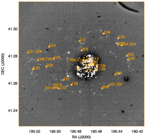
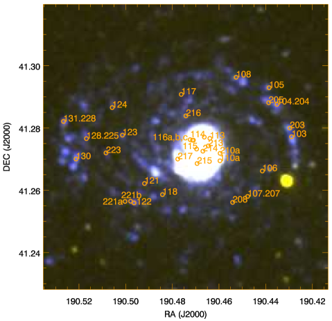
Figure 1: Left: Continuum-subtracted H$\alpha$ image of NGC 4625, obtained from our Subaru FOCAS imaging. Right: GALEX UV colour composite image of NGC 4625. Our H ii region sample is shown by the orange circles marked with the object IDs.

We measured the spectral line strengths by direct integration of the flux measured between two continuum regions interactively selected on each side of the line. The reddening correction was done using the extinction curve published by Osterbrock (1989), and assuming an intrinsic H$\gamma$/H$\beta$ ratio of 0.47, which holds at T_e = $10^{4}$ K. We were unable to use the H$\alpha$/H$\beta$ ratio because these two Balmer lines appear separately in the red and blue spectra, respectively. Therefore, the theoretical ratio H$\alpha$/H$\beta$ $=2.86$ was adopted to renormalise the line fluxes in the red spectral range, after we had made the reddening correction. The line flux ratios that involve emission features observed separately in the blue and red spectra could potentially be affected by the variations in the seeing conditions mentioned earlier. Fortunately, the spectra for our second mask were obtained with an approximately constant image quality ($\sim 1"$). Moreover, since a few of the targets were included in both masks, we could verify that the flux ratios did not suffer from changes in the seeing.

Table 2: Reddening-corrected lines fluxes.

ID	[O ii]	[O iii]	[N ii]	[S ii]	[Ar iii]	F(H$\beta$) / $10^{-16}$	c(H$\beta$)	$\log\frac{\mbox{[N\,{\sc ii}]}}{\mbox{[O\,{\sc ii}]}}$	$\log\frac{\mbox{[N\,{\sc ii}]}}{\mbox{H}\alpha}$
	3727	5007	6583	6717+6731	7135	(erg s-1 cm-2)
(1)	(2)	(3)	(4)	(5)	(6)	(7)	(8)	(9)	(10)
103	$311\pm 21$	$92\pm 4$	$29\pm 1$	$67\pm 2$	$4\pm 0.9$	3.2	$0.00\pm 0.20$	$-1.02$	$-0.98$
104.204	$344\pm 16$	$122\pm 5$	$28\pm 1$	$43\pm 1$	$6\pm 0.6$	3.9	$0.00\pm 0.14$	$-1.08$	$-1.00$
105	$295\pm 25$	$158\pm 7$	$24\pm 1$	$37\pm 2$	$7\pm 1.3$	2.4	$0.00\pm 0.20$	$-1.08$	$-1.07$
106	$291\pm 38$	$337\pm 19$	$26\pm 3$	$49\pm 5$	$18\pm 3.6$	1.0	$0.00\pm 0.29$	$-1.05$	$-1.04$
107.207	$333\pm 40$	$158\pm 10$	$41\pm 4$	$61\pm 5$	…	0.6	$0.00\pm 0.29$	$-0.90$	$-0.84$
108	$266\pm 16$	$414\pm 19$	$26\pm 1$	$68\pm 2$	$9\pm 1.0$	4.4	$0.00\pm 0.17$	$-1.01$	$-1.04$
110a	$148\pm 25$	$20\pm 1$	$98\pm 2$	$78\pm 1$	$4\pm 0.1$	17.2	$0.16\pm 0.16$	$-0.18$	$-0.46$
113	$139\pm 21$	$25\pm 1$	$96\pm 2$	$40\pm 1$	$7\pm 0.2$	17.7	$0.96\pm 0.18$	$-0.16$	$-0.47$
114	$155\pm 12$	$24\pm 1$	$97\pm 1$	$67\pm 1$	$4\pm 0.1$	53.8	$0.08\pm 0.13$	$-0.20$	$-0.47$
115	$100\pm 22$	$33\pm 3$	$121\pm 4$	$56\pm 1$	$7\pm 0.4$	10.0	$0.38\pm 0.32$	$\phantom{-}0.09$	$-0.37$
116a	$119\pm 15$	$14\pm 1$	$99\pm 2$	$82\pm 1$	$3\pm 0.4$	20.3	$0.59\pm 0.20$	$-0.08$	$-0.46$
116b	$179\pm 16$	$35\pm 1$	$107\pm 2$	$68\pm 1$	$4\pm 0.2$	22.3	$0.62\pm 0.16$	$-0.22$	$-0.42$
116c	$178\pm 16$	$109\pm 5$	$104\pm 2$	$58\pm 1$	$10\pm 0.2$	17.0	$0.89\pm 0.16$	$-0.23$	$-0.44$
117	$277\pm 36$	$284\pm 33$	$29\pm 3$	$40\pm 3$	$13\pm 2.9$	1.1	$0.00\pm 0.30$	$-0.97$	$-0.99$
118	$315\pm 72$	$204\pm 11$	$38\pm 1$	$53\pm 1$	$9\pm 0.3$	3.9	$0.04\pm 0.20$	$-0.91$	$-0.87$
121	$395\pm 103$	$204\pm 23$	$39\pm 2$	$61\pm 3$	…	1.0	$0.13\pm 0.44$	$-1.00$	$-0.86$
122	$268\pm 54$	$167\pm 15$	$31\pm 1$	$55\pm 2$	$7\pm 0.5$	2.3	$0.43\pm 0.34$	$-0.93$	$-0.96$
123	$319\pm 47$	$39\pm 5$	$34\pm 3$	$82\pm 4$	…	1.4	$0.00\pm 0.41$	$-0.97$	$-0.92$
124	$309\pm 60$	$209\pm 18$	$31\pm 1$	$63\pm 2$	$8\pm 0.6$	1.5	$0.09\pm 0.33$	$-1.00$	$-0.96$
128.225	$379\pm 56$	$36\pm 2$	$31\pm 2$	$106\pm 4$	…	1.3	$0.00\pm 0.25$	$-1.08$	$-0.96$
130	$274\pm 20$	$146\pm 6$	$19\pm 1$	$44\pm 2$	$6\pm 1.7$	3.0	$0.00\pm 0.18$	$-1.15$	$-1.17$
131.228	$378\pm 82$	$62\pm 6$	$29\pm 1$	$76\pm 3$	…	4.4	$1.30\pm 0.39$	$-1.10$	$-0.98$
203	$334\pm 31$	$196\pm 11$	$27\pm 2$	$69\pm 4$	…	1.7	$0.00\pm 0.29$	$-1.08$	$-1.01$
205	$181\pm 25$	$397\pm 17$	$17\pm 2$	$23\pm 3$	$14\pm 1.2$	1.5	$0.00\pm 0.21$	$-1.02$	$-1.21$
208	$357\pm 38$	$64\pm 4$	$47\pm 3$	$155\pm 7$	…	1.3	$0.00\pm 0.24$	$-0.88$	$-0.78$
210a	$168\pm 16$	$44\pm 2$	$91\pm 2$	$91\pm 1$	$7\pm 0.2$	8.2	$0.08\pm 0.17$	$-0.26$	$-0.49$
213	$202\pm 9$	$30\pm 1$	$105\pm 4$	$74\pm 2$	$5\pm 0.3$	18.9	$0.00\pm 0.13$	$-0.28$	$-0.43$
214	$149\pm 9$	$28\pm 2$	$96\pm 4$	$83\pm 3$	$5\pm 0.9$	14.4	$0.00\pm 0.21$	$-0.19$	$-0.47$
215	$225\pm 17$	$54\pm 2$	$112\pm 2$	$149\pm 2$	$8\pm 0.2$	5.7	$0.40\pm 0.14$	$-0.30$	$-0.41$
216	$230\pm 32$	$256\pm 13$	$68\pm 3$	$104\pm 4$	$10\pm 2.1$	2.6	$0.00\pm 0.19$	$-0.53$	$-0.62$
217	$192\pm 8$	$76\pm 3$	$73\pm 3$	$58\pm 2$	$8\pm 0.5$	31.7	$0.00\pm 0.13$	$-0.42$	$-0.59$
221a	$359\pm 98$	$164\pm 19$	$43\pm 2$	$75\pm 3$	…	1.2	$0.27\pm 0.44$	$-0.92$	$-0.82$
221b	$353\pm 43$	$75\pm 6$	$31\pm 4$	$84\pm 6$	…	0.9	$0.00\pm 0.32$	$-1.05$	$-0.96$
223	$357\pm 88$	$55\pm 6$	$39\pm 2$	$87\pm 3$	…	2.9	$0.58\pm 0.39$	$-0.95$	$-0.86$

Line fluxes are normalized to H$\beta=100$. The H$\beta$ flux in col. 7 is uncorrected for potential slit losses.

We list the reddening-corrected line fluxes of our sample, in units of H$\beta=100$, in Table 2. The quoted errors account for measurement, flux calibration and flat fielding errors. We point out that the H$\beta$ flux (column 7) underestimates the total line flux (hence the ionizing luminosity, see §4.2.1), due to the unavoidable slit losses.

We have characterised our H ii region sample using the familiar BPT (Baldwin et al., 1981) diagnostic diagrams, by plotting in Fig. 2 [N ii]/H$\alpha$ against [O iii]/H$\beta$ and [S ii]/H$\alpha$ against [O iii]/H$\beta$ (Veilleux & Osterbrock, 1987). We represent our sample of H ii regions with orange triangle symbols, and we include comparison data of mostly bright extragalactic H ii regions drawn from the literature:

1.

99 H ii regions measured in 20 spiral and irregular galaxies by McCall et al. (1985, dark grey dots).

2.

198 H ii regions in 13 spiral galaxies from van Zee et al. (1998, grey dots).

3.

17 H ii regions from three late-type spirals (NGC 628, NGC 1058 and NGC 6946) studied by Ferguson et al. (1998a, light grey dots).

4.

41 H ii regions in the spiral galaxy M101 observed by Kennicutt & Garnett (1996, black dots).

5.

16 H ii regions from the inner disc of M83 from Bresolin & Kennicutt (2002, dark blue squares).

6.

49 H ii regions from the M83 sample of Bresolin et al. (2009a, light blue squares), mostly composed of outer disc H ii regions. Note that the two objects which appear above the theoretical boundary in Fig. 2 were identified as supernova remnants.

H ii regions in the inner disc of NGC 4625 are further identified by green dots, while the outer disc H ii regions are marked either with cyan dots, indicating [O iii]$\,\lambda\lambda$4959, 5007/H$\beta>0.25$, or red dots ([O iii]$\,\lambda\lambda$4959, 5007/H$\beta<0.25$). This arbitrary distinction helps us to distinguish these two subsets. In fact, in the [N ii]/H$\alpha$ vs. [O iii]/H$\beta$ diagram not all of the inner disc H ii regions sit on the tight sequence defined by bright H ii regions: those marked with red dots appear to lie below and/or to the left of the main ionisation sequence. On the other hand, the [S ii]/H$\alpha$ versus [O iii]/H$\beta$ plot shows a similar ionisation sequence for objects in the inner and extended disc of NGC 4625, which is consistent with the ionisation sequence defined by bright extragalactic H ii regions. These results will be further discussed in §4.

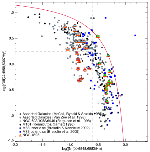
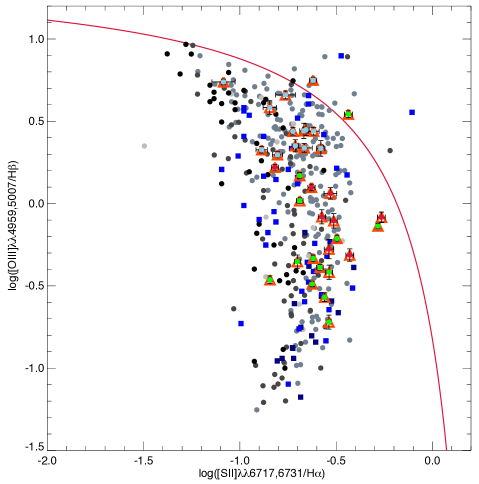
Figure 2: BPT diagnostic plots. Left: [O iii]/H$\beta$ vs. [N ii]/H$\alpha$. Right: [O iii]/H$\beta$ vs. [S ii]/H$\alpha$. Our sample of H ii regions in NGC 4625 (triangles) has been plotted together with published H ii region datasets. Objects in the inner disc are further identified by green dots, while the outer disc H ii regions are marked either with cyan dots, indicating [O iii]/H$\beta>0.25$, or red dots for [O iii]/H$\beta<0.25$. The blue squares show the H ii regions observed in the other prototypical XUV galaxy, M83, with light blue squares representing the outer disc sample of Bresolin et al. (2009a), and dark squares the inner disc H ii regions of Bresolin & Kennicutt (2002). The dots show previous studies of bright inner disc H ii regions, including the samples of McCall et al. (1985, dark grey dots) and van Zee et al. (1998, grey dots). The light grey dots represent the H ii regions in NGC 628, NGC 1058 and NGC 6946 studied by Ferguson et al. (1998a). The M101 sample of Kennicutt & Garnett (1996) is represented by the black dots. The red curves represent the upper boundaries for photoionised nebulae defined by Kewley et al. (2006). The dashed lines in the left panel serve to schematically isolate objects that appear to deviate from the main ionisation sequence, towards the lower left of the diagram.

Eight of our H ii regions were also studied by G07 (identified in Table 1 by the xuv numbers used in their paper). The H$\beta$ fluxes measured by G07 are systematically higher than ours by a mean factor of 1.45, as expected from their 50% larger slit widths (1$\aas@@fstack{\prime\prime}$5 vs. 1$\aas@@fstack{\prime\prime}$0), and thus it appears that the poor seeing conditions that we experienced did not significantly affect our flux measurements. Our [O iii]/H$\beta$ ratios for 6 H ii regions in common (not all of the G07 had a measured [O iii] line) are systematically 22% lower, on average, for which we do not have an explanation. Of the only four targets for which the intensity of the [O ii]$\,\lambda$3727 line could be compared, we found good agreement in two cases (our regions 118 and 122), a 34% lower flux ratio in a third (region 103), which is mostly due to our lower assumed reddening correction, while in the case of region 130 our [O ii]/H$\beta$ value is almost a factor of 2 lower. In this last case, the reddening correction cannot explain the large discrepancy. It is well-known (e.g. Bresolin et al. 2005) that the [O ii]$\,\lambda$3727 line is susceptible to systematic errors in nebular optical spectra, as a result of the increased uncertainty in the flux calibration of the blue end of the spectrum, smaller throughput at these wavelengths, and errors in the reddening corrections. We conclude by noting that most of the spectra shown in Fig. 4 of G07 are very noisy in the region around 4000 Å, and in several cases even the H$\beta$ line seems to be detected with a poor signal-to-noise ratio (unfortunately G07 did not publish error estimates for their line ratios, so this statement is based on a visual assessment of their data). Thanks to longer exposure times (2 hours vs. 40 minutes) with a larger telescope aperture (Subaru 8 m vs. Palomar 5 m), our spectra are, as should be expected, of superior quality. We are therefore confident in the reliability of our emission line data and the estimated uncertainties presented in Table 2.

3 Nebular Abundances

Table 3: Auroral line-derived abundances.

ID	[O iii]$\,\lambda$4363/H$\beta$	Te (K)	12 + log(O/H)	log(N/O)
(1)	(2)	(3)	(4)	(5)
104.204	$2.0\pm 1.5$	$14000\pm 2700$	$7.95\pm 0.32$	$-1.09\pm 0.34$
108	$8.2\pm 1.4$	$15300\pm 1100$	$8.01\pm 0.09$	$-1.27\pm 0.12$
205	$7.7\pm 4.2$	$15100\pm 2500$	$7.93\pm 0.25$	$-1.35\pm 0.31$

3.1 Direct Abundances

Ideally, the derivation of the chemical abundances of ionised nebulae requires first a measurement of the electron temperature T_e, since the line emissivities strongly depend on it. The classical method to directly obtain T_e involves the simultaneous measurement of the auroral [O iii]$\,\lambda$4363 line and of the nebular [O iii]$\,\lambda\lambda$4959, 5007 lines. This proves to represent a challenge with the increase of the metallicity, because the cooling mechanisms become highly efficient and [O iii]$\,\lambda$4363 too weak to observe. However, having a few $\,\lambda$4363 detections is important, since they allow the derivation of nebular abundances that are independent of the systematic uncertainties of the strong line methods described below. In our NGC 4625 sample three H ii regions were found to have a reliable [O iii]$\,\lambda$4363 detection. With routines in the iraf nebular package we obtained T_e and subsequently the O/H and N/O ratios, assuming that N/O = N⁺/O⁺. These quantities are summarised in Table 3.

3.2 Strong Line Abundances

Without detection of the temperature-sensitive [O iii]$\,\lambda$4363 line we must resort to strong line methods to determine the oxygen abundances. Several such methods, using a variety of line ratios, are present in the literature, with calibrations that are provided either empirically or by theoretical considerations. Unfortunately, it is well established that the various methods provide differing solutions for the chemical composition of star forming galaxies and H ii regions, resulting in systematic shifts of up to $\sim$0.7 dex (Kewley & Ellison, 2008; Bresolin et al., 2009b). By providing the reader with results from different strong line indicators we hope to detect any robust trends in the abundance gradient of NGC 4625, and at the same time highlight the limitations of our findings. Although these indicators were originally developed for the study of the chemical abundances of luminous extragalactic H ii regions, tests on Galactic nebulae ionised by single or only a few stars have excluded the presence of systematic effects (Kennicutt et al., 2000; Oey & Shields, 2000). Further empirical tests were carried out by our team when analysing a set of faint outer disc H ii regions in M83 (Bresolin et al., 2009a).

We have considered the following strong line abundance indicators in the remainder of our work:

1.

R₂₃ = ([O ii]$\,\lambda$3727 + [O iii]$\,\lambda\lambda$4959, 5007)/H$\beta$. This is one of the most widely used strong line abundance indicators, however it does have some limitations (e.g. Pérez-Montero & Díaz, 2005). In particular, the R₂₃ indicator has a double valued nature, peaking with a value log(R₂₃) $\simeq$ 1 around 12 + log(O/H) = 8.5 in the theoretical calibration provided by McGaugh (1991). Smaller R₂₃ values correspond to both lower and higher O/H abundances. The turnover occurs at lower abundances, 12 + log(O/H) $\simeq$ 8.0, when using O/H empirical determinations from [O iii]$\,\lambda$4363 detections (Bresolin 2007, 2008). Because of this degeneracy, it is essential to establish whether the H ii regions under scrutiny fall into the lower or upper R₂₃ branch. This is commonly accomplished with the help of line ratios that vary monotonically with metallicity, such as [N ii]/H$\alpha$ and [N ii]/[O ii].

2.

N2 = [N ii]$\,\lambda$6583/H$\alpha$, as empirically calibrated by Pettini & Pagel (2004). N2 is a monotonic function of the oxygen abundance and thus avoids the degeneracy problem associated with R₂₃. However, Kewley & Dopita (2002,  = KD02) showed that N2 is sensitive to the ionisation parameter.

3.

N2O2 = [N ii]$\,\lambda$6583/[O ii]$\,\lambda$3727, a useful indicator because it is highly insensitive to the ionisation parameter (Dopita et al., 2000). We have used two separate calibrations in this study, the theoretical one by KD02, based on grids of photoionisation models, and the empirical one by Bresolin (2007,  = B07), based on a sample of H ii regions with available T_e abundances.

We note that N2 and, to a lesser extent, R₂₃ are more robust against uncertainties in the atmospheric extinction correction compared to the N2O2 indicator, which is formed by emission lines spread across a very wide spectral range. N2, in particular, is also virtually insensitive to uncertainties in the interstellar reddening correction and to the potential effects of variable seeing, which could be significant for flux ratios that involve emission lines measured from separately obtained blue and red spectra, as is often the case for [N ii]/[O ii].

3.2.1 Results

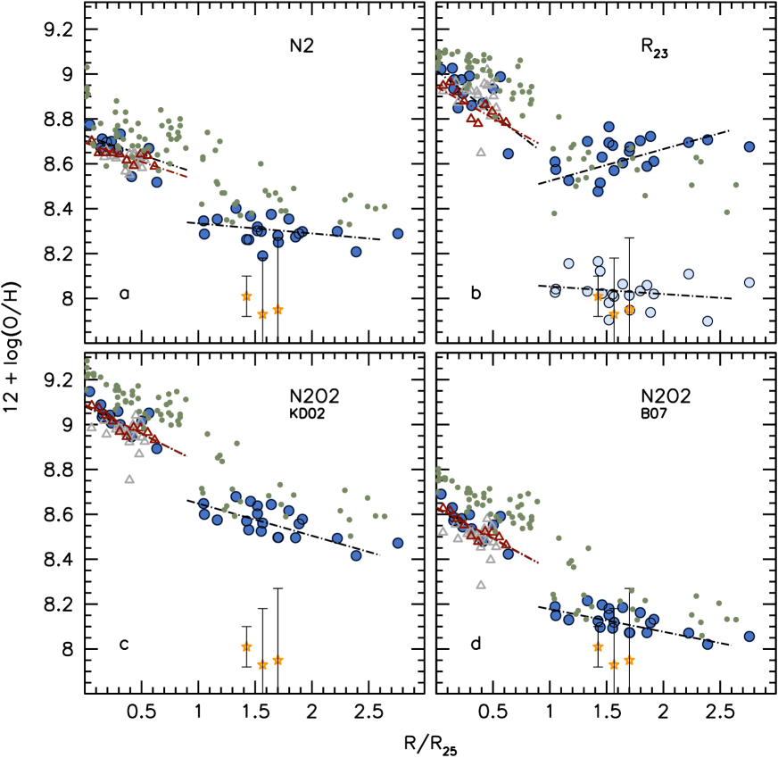
Figure 3: The radial oxygen abundance gradient in NGC 4625 (coloured circles), determined using various strong line methods: (a) N2, calibrated by Pettini & Pagel (2004); (b) R₂₃, with upper branch calibration shown in blue, and lower branch calibration in light blue; (c) N2O2, theoretical calibration by Kewley & Dopita (2002); (d) N2O2, empirical calibration by Bresolin (2007). T_e-based abundances have been added to all four panels as gold star symbols. We include the results obtained from measurements of the inner disc from the PINGS survey, including individual H ii regions studied in our sample (grey triangles) and radially averaged abundances (red triangles). For comparison, the M83 data points from Bresolin et al. (2009a) are shown by the green dots. The lines represent weighted least square fits to our Subaru data for the inner and outer disc (black) and to the radially averaged PINGS data (red).

Table 4: Coefficients of least-squares fitting to the relation 12 + log(O/H) =  $a-b$ (R/R₂₅).

	Abundance	Inner Disc		Outer Disc
	Indicator	$a$	$b$	$a$	$b$
Our Sample	N2	$8.72\pm 0.03$	$-0.17\pm 0.08$	$8.38\pm 0.03$	$-0.05\pm 0.02$
	R23 (upper branch)	$9.02\pm 0.04$	$-0.39\pm 0.13$	$8.38\pm 0.08$	$+0.14\pm 0.05$
	R23 (lower branch)	–	–	$8.09\pm 0.07$	$-0.03\pm 0.03$
	N2O2 (KD02)	$9.08\pm 0.02$	$-0.25\pm 0.08$	$8.79\pm 0.06$	$-0.14\pm 0.04$
	N2O2 (B07)	$8.63\pm 0.02$	$-0.27\pm 0.08$	$8.28\pm 0.04$	$-0.10\pm 0.03$
PINGS	N2	$8.69\pm 0.01$	$-0.17\pm 0.03$	–	–
(Radial data)	R23 (upper branch)	$8.94\pm 0.04$	$-0.28\pm 0.08$	–	–
	N2O2 (KD02)	$9.09\pm 0.02$	$-0.26\pm 0.04$	–	–
	N2O2 (B07)	$8.63\pm 0.02$	$-0.27\pm 0.05$	–	–

In Fig. 3 we present the abundances we derived from the strong line indicators, plotted as a function of galactocentric distance. The three targets with T_e-based abundances appear as gold stars. We show with black dot-dashed lines the weighted least squares fits to the data for both the inner (R $<$ R₂₅) and outer (R $>$ R₂₅) disc. We also include as a comparison the sample of M83 H ii regions studied by Bresolin et al. (2009a, green dots), further discussed in §3.2.2.

The triangles in Fig. 3 represent measurements of H ii regions in NGC 4625 from PINGS (PPAK Integral Field Spectroscopy Nearby Galaxy Survey, see Rosales-Ortega et al. 2010), which obtains spectra from the PMAS integral field unit at the Calar Alto 3.5 m telescope. To compare the PINGS results to our own we followed two different approaches, either by averaging spectra from all fibers contained within equally spaced ($4^{\prime\prime}$ separation) radial bins (red triangles in Fig. 3), or by using the sum of individual fibers covering the spatial extent of individual H ii regions (grey triangles). The agreement between the abundances derived from PINGS and our data is excellent, as shown by the close match between the regressions to the average radial bins (red lines) and to our inner disc results (black). This can be quantitatively appreciated by looking at the coefficients of the weighted linear fits to the the radial trends of metallicity that are summarized in Table 4.

Following is a brief discussion of the results obtained from the individual abundance diagnostics:
R₂₃ – The interpretation of the R₂₃-based abundances (top right-hand panel of Fig. 3) requires some important considerations. All the inner disc H ii regions in NGC 4625 have log ([N ii]/H$\alpha$) $>$ $-0.8$, which, according to the KD02 photoionisation models, corresponds to the upper branch of R₂₃. The result could be more ambiguous for the outer disc H ii regions, which are closer to the turnover region in the R₂₃ vs. metallicity relationship, even though virtually all lie in the upper-branch regime, according to the Kewley & Ellison (2008) criterion, log ([N ii]/H$\alpha$) $>$ $-1.1$. We reach the same conclusion from the log ([N ii]/[O ii]) values (ranging between $-1.1$ and $-0.7$). Therefore, we used the upper branch solution for the inner disc, whilst for the outer disc we used both the lower branch (light blue) and the upper branch (dark blue) calibrations of McGaugh (1991, in the analytical form given by ) for comparison.

Taking at face value the information obtained from the [N ii]/H$\alpha$ and [N ii]/[O ii] line ratios we would be led to favour the upper branch solution for the whole sample of H ii regions, leading, in particular, to 12 + log(O/H) $\sim$ 8.6 in the outer disc. However, this is in evident contrast with the direct abundances that we measured for the three outer disc targets presented in Table 3. Their oxygen abundance, 12 + log(O/H) $\sim$ 8.0, agrees very well with the lower branch solution shown in Fig. 3. This inconsistency is the result of the still unresolved discrepancy between theoretical and direct calibrations of strong-line indicators. We note that our measurements for the direct abundances essentially fall in the transition range 12 + log(O/H) =8̇.0 - 8.25 between upper and lower branch of the R₂₃ calibration based on the P-parameter of Pilyugin & Thuan (2005), which is directly tied to the empirical, [O iii]$\,\lambda$4363-based oxygen abundances. Consequently, we cannot obtain a reliable estimate of the outer disc abundances from this method, although clearly they would be systematically lower than those from the theoretical McGaugh (1991).

N2 – We point out that this diagnostic, when applied to the three targets with a $\,\lambda$4363 detection, provides abundances that are 0.3 dex higher relative to the direct method (top left-hand panel of Fig. 3). This is not fully expected, since the N2 calibration by Pettini & Pagel (2004) relies mostly on extragalactic H ii regions where the oxygen abundances had been derived from auroral line detections However, a similar effect was observed in M83 by Bresolin et al. (2009a). We can speculate on the possible causes of this systematic difference, pointing out that the the ionization properties of the calibration sample can differ significantly from those of the faint nebulae found in the extended discs, and that the N2 diagnostic is sensitive to variations in the ionization parameter (KD02).

N2O2 – The lower right-hand panel of Fig. 3 shows the strong line abundances calculated with the calibration of the [N ii]/[O ii] vs. O/H relation by Bresolin (2007). Unsurprisingly, this indicator provides a good match, within the uncertainties, to the direct T_e-based abundances, since the calibration was empirically derived from extragalactic H ii regions with auroral line detections. The well-known systematic discrepancies associated with the use of different strong line indicators and their calibration are evident in Fig. 3. The theoretical N2O2 calibration of Kewley & Dopita (2002) yields abundances that are roughly 0.45 dex higher than the empirical calibration of Bresolin (2007). Similar systematic shifts are present between N2 and N2O2.

3.2.2 What do the Strong Line Abundances Reveal?

Despite the systematic offsets between different abundance diagnostics noted above, the results summarised in Fig. 3 appear to be qualitatively consistent with each other, in particular showing a shallower gradient in the outer disc, as well as an abundance discontinuity between the inner and outer disc, occurring near R₂₅. Extrapolation of the inner and outer disc abundance gradients suggests a discontinuity of approximately 0.15-0.2 dex, based on the N2 and N2O2 abundance indicators. As Table 4 shows, the slopes of the gradients depend somewhat on the choice of abundance indicator. In the inner disc, N2 produces the flattest gradient ($-0.17$ dex/R₂₅), about half of the value obtained from R₂₃ ($-0.39$ dex/R₂₅). The scatter of the data points is, however, quite large in the R₂₃ case. If we look at the radially averaged PINGS data we find a good agreement between R₂₃ and N2O2 ($\sim$ $-0.27$ dex/R₂₅), still slightly larger (2 $\sigma$) than the slope provided by N2. The outer disc slopes are also smaller (1 $\sigma$) for N2 ($-0.05$ dex/R₂₅) than for N2O2 ($-0.10$ to $-0.14$  dex/R₂₅). This agrees with the conclusion by Bresolin et al. (2009b) in their detailed study of NGC 300 that abundance gradient slope values have a dependency on the method adopted to measure them, contrary to other statements in the literature, that changing the strong-line abundance calibration only affects the zero points.

We include in Fig. 3 the data on the inner and outer H ii regions in M83 analyzed by Bresolin et al. (2009a, green dots). This allows us to compare the results we obtained for NGC 4625 to the only other extended disc galaxy studied in detail until now. As the figure shows, there is a very good qualitative match between the two galaxies. The change in the galactocentric abundance slope between inner and outer disc is comparable, as is the discontinuity in O/H detected around the isophotal radius, as well as the slope of the gradients themselves. The outer discs in the two galaxies have remarkably similar oxygen abundances, regardless of the metallicity indicator used for the comparison. The inner disc abundances in M83 are $\sim$0.15 dex higher than in the case of NGC 4625, which is, at least qualitatively, expected from the higher absolute luminosity of the former ($M_{B}=-20.8$ vs. $M_{B}=-17.2$ adopting distances of 4.5 and 9.5 Mpc, respectively). Panel (b) of Fig. 3 also suggests that the apparent positive abundance gradient obtained in the outer disc of NGC 4625 from the use of the upper branch of R₂₃ could be due to small number statistics at large radius, since the scatter of the points is similar for the two galaxies, and M83 does not show a positive gradient in its outer parts. This would imply that the R₂₃-inferred change of slope between inner and outer disc of NGC 4625 would be made roughly consistent with what is observed with the other diagnostics.

4 Analysis of the H II Region Sample

Earlier on (Fig. 2) we showed the familiar BPT diagnostic diagrams for our sample in NGC 4625, concluding that all objects were indeed photoionized nebulae. However, these plots also revealed a subset of outer disc H ii regions which apparently lie off the main ionisation sequence defined by extragalactic giant H ii regions in the [N ii] vs. [O iii] plane, whilst apparently conforming to the less robust sequence formed in the [S ii] vs. [O iii] plane.

4.1 Properties of H II Regions in the Outer Disc

We have arbitrarily subdivided the outer disc H ii regions in NGC 4625 by making a cut at [O iii]/H$\beta=0.25$, represented in Fig. 2 with a horizontal dashed line. The outer H ii regions which lie on the tight, well defined ionisation sequence shown in the left panel of Fig. 2 fall above our cut and are highlighted with central cyan dots. Those which lie off the ionisation sequence and below our [O iii]/H$\beta$ cut were marked with red dots. It is not obvious whether the latter deviate as a result of either a smaller [N ii] or a smaller [O iii] emission (or both) relative to the sequence defined by bright H ii regions. We note that a few of the outer disc objects in M83, as well as a small number of nebulae in other galaxies, also lie below and to the left of the ionisation sequence.

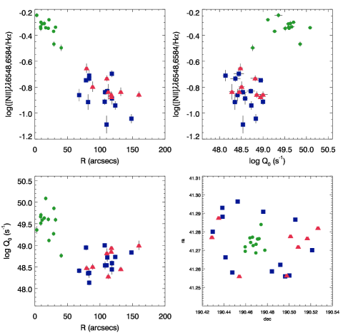
Figure 4: Properties of outer disc H ii regions, for objects with [O iii]/H$\beta>0.25$ (blue squares) and [O iii]/H$\beta<0.25$ (red triangles) marked separately. Top-left: [N ii]/H$\alpha$ vs. galactocentric distance. Top-right: [N ii]/H$\alpha$ as a function of ionising luminosity. Bottom-left: ionising luminosity as a function of galactocentric distance. Bottom-right: spatial distribution of individual H ii regions. Inner disc H ii regions are indicated by the green dots.

It is worth testing whether these apparently deviant H ii regions share any common attributes, such as ionising luminosity, spatial distribution, metallicity and so forth. This is done in Fig. 4. The top-left panel shows the [N ii]/H$\alpha$ line ratio, i.e. the N2 chemical abundance indicator, as a function of galactocentric radius. No differential behaviour between the two groups of outer disc H ii regions (blue and red symbols) is evident. The two groups also appear to share similar ionising luminosities (upper right and lower left panels) and to be evenly distributed throughout the XUV disc of NGC 4625, without the presence of obvious separate sub-structures (lower right). There are slight indications that the deviant H ii regions have a systematically higher [N ii]/H$\alpha$ line ratio than the other outer disc H ii regions, but this could easily be explained by the variance of the two distributions.

4.2 Systematics in the Diagnostic Diagrams

In the following we consider what might affect the line fluxes in such a way as to produce the observed deviation of a small number of outer disc H ii regions from the main ionisation sequence in the BPT diagnostic diagram.

4.2.1 Stochastic Variations

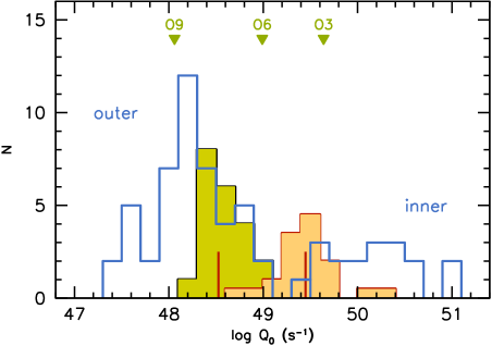
Figure 5: Histograms of the H ionising photon flux, $\rm Q_{0}$, of H ii regions in our sample, uncorrected for slit losses. The green and orange shaded areas represent H ii regions in the outer and inner disc of NGC 4625, respectively. We have marked the median values for the two populations (log $\rm Q_{0}$ = 48.52 and 49.45, respectively). The blue lines show the histogram of the M83 sample studied by Bresolin et al. (2009a). The triangles at the top represent reference $\rm Q_{0}$ values for single hot stars (O3, O6 and O9), from Martins et al. (2005).

The direct observation of the ionising population of nebulae in outer galaxy discs are extremely difficult, thus the properties of the associated stellar clusters have so far been obtained from studies of their H$\alpha$ and UV luminosities (Gil de Paz et al., 2005, 2008; Goddard et al., 2010), together with their IR emission (Dong et al., 2008). The total ionising photon flux of individual clusters can be easily estimated from the H$\alpha$ luminosity, using the conversion given by Kennicutt (1998). In Fig. 5 we show histograms of the hydrogen ionising photon flux for both the inner (orange) and outer (green) disc H ii regions, along with their median values. As a reference, we also show the hydrogen ionising fluxes of O3, O6 and O9 dwarf stars, taken from Martins et al. (2005). The luminosities that we measure do not account for slit losses, which are expected to be smaller for the outer disc H ii regions, given that a greater percentage of their flux will fall through the 1^′′ slits compared to the brighter and larger inner disc H ii regions. We estimated the slit losses by measuring H ii region fluxes on an H$\alpha$ image of NGC 4625 provided by the SINGS survey (Kennicutt et al., 2003). In the case of the faintest H ii regions losses are in the 5-10% range, while for the brighter inner H ii regions they increase to 20-70%.

Figure 5 confirms what other authors already found, namely that that the inner disc sample of H ii regions is brighter than the outer disc population by at least one order of magnitude (more if slit losses were considered). The ionising flux of typical outer disc H ii regions corresponds to that of a single late-type O star (see Gil de Paz et al. 2005; Thilker et al. 2005; Dong et al. 2008; Goddard et al. 2010). Consequently, it is necessary to account for the stochastic nature of the upper Initial Mass Function (IMF) of the ionizing clusters. An ionising population drawn from a stochastically sampled IMF, as opposed to a fully sampled one, will tend to have a lower effective temperature, due to the preferential depletion of the rarest, most massive main sequence stars. This has important consequences for the total ionizing flux output, as well as for the hardness of the ionizing radiation. In particular, as a result of softer spectral energy distributions, line ratios involving both high- and low-ionization potential species could be significantly affected.

4.2.2 Age effects

As the ionizing population of an H ii region ages the most massive stars die first, effectively truncating the mass function of the remaining stellar population. Not only could this alter the emission line fluxes, but we can also think of this effect as a proxy for stochastic variations which, as we have just seen, also act in the send of removing the high mass end of the stellar population.

We make a simple attempt to model such age effects by using the itera program (Groves & Allen, 2010), along with the starburst models of Levesque et al. (2010), which adopt a Salpeter IMF and the Starburst99 (Leitherer et al. 1999) stellar spectral energy distributions with standard mass loss rates. In Fig. 6 we show a set of models on the [O iii]/H$\beta$ vs. [N ii]/H$\alpha$ diagnostic diagram, calculated for a range of metallicities (Z = 0.2, 0.4, and 1.0 $Z_{\odot}$), ionisation parameters (Q₀ = $2\times 10^{7}$, $8\times 10^{7}$, and $4\times 10^{8}$) and ages (t = 0, 3, 5, 6 Myr). The H ii region samples introduced in §2 are represented by the grey dots, whilst our targets in NGC 4625 are shown either with cyan ([O iii]/H$\beta>0.25$) or green ([O iii]/H$\beta<0.25$) symbols.

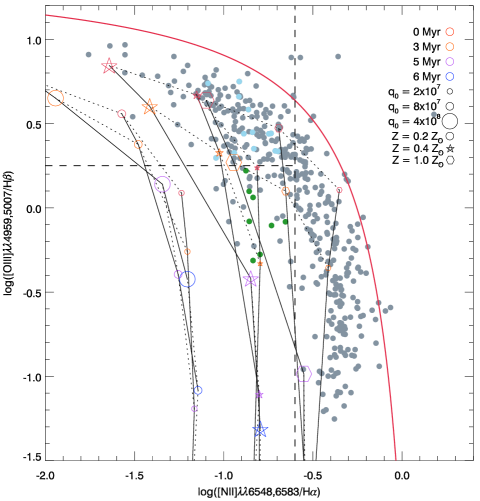
Figure 6: Models in the [O iii]/H$\beta$ vs. [N ii]/H$\alpha$  diagnostic diagram. The grey dots represent the same extragalactic H ii region samples included in previous figures. Cyan symbols are used for outer disc H ii regions in NGC 4625 for which [O iii]/H$\beta>0.25$, whilst green dots are used for those with [O iii]/H$\beta<0.25$. The red line represents the upper boundary for photoionised nebulae defined by Kewley et al. (2006). Black lines link models with identical ionisation parameter, whilst the dotted lines link models of the same age.

The zero-age models in Fig. 6 lie on top of the ionisation sequence defined by the main extragalactic sample of giant H ii regions. The models show that, as the H ii regions evolve with time after the initial burst of star formation, the [O iii] emission rapidly decreases, and the good match with the observational data quickly disappears (see earlier results by Bresolin et al. 1999). The models also depart from the main ionisation sequence to lower [N ii]/H$\alpha$ values as the metallicity decreases. The best fit to our deviant H ii regions (green dots) is obtained with the 0.4 $Z_{\odot}$ models and ages between 3 and 5 Myr, depending on the ionisation parameter.

The model comparison offers some clues as to why some H ii regions appear to deviate from the main ionisation sequence. Our interpretation relies on the fact that, as mentioned earlier, the evolution of the ionising output of low-luminosity H ii regions with age can mimic the effects due to stochastic variations in the number of ionizing stars. One might ask why so few H ii regions have been seen with similar properties in previous studies. The reasons are two-fold. Firstly, most of the previous studies have focused on inner disc H ii regions, which tend to have higher metallicities. According to our models, these objects would be nearly superimposed onto the main ionisation sequence. Secondly, there is a selection effect at work, since in the inner discs the brightest and youngest H ii regions are preferentially studied, also as a result of source confusion and crowding near the central regions and along the spiral arms, while in the outer disc we attempt to sample as many H ii regions as possible, even the faintest ones, thus probing to older ages. This conclusion could be tested with spectroscopic observations of larger samples of inner disc H ii regions, reaching to fainter emission levels.

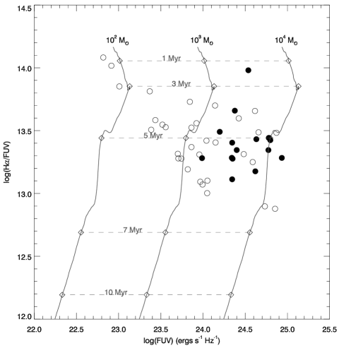
Figure 7: FUV/H$\alpha$ ratio as a function of FUV luminosity for XUV disc objects in NCG 4625 as measured by Goddard et al. (2010). Objects for which an H ii region in our sample falls under the area of a UV-detected object are shown as filled circles. Open circles are used in cases where we have instead measured the total H$\alpha$ emission coming from a region that matches in size the UV-identified objects. Grey lines show theoretical Starburst99 models for three cluster masses (10², $10^{3}$ and $10^{4}$ $M_{\odot}$). Dashed lines connect models of constant age.

We estimated the ages of the H ii regions in our sample by looking at the UV and H$\alpha$ fluxes measured by Goddard et al. (2010). In Fig. 7 we plot the FUV/H$\alpha$ ratio as a function of the FUV luminosity. We have marked with filled circles those objects for which an H ii region matches the position of an identified FUV object. For the remaining cases (open circles) we have measured the total H$\alpha$ emission coming from a region that matches in size the UV-identified objects. We include Starburst99 models calculated for a single burst of star formation at three different cluster masses (10², $10^{3}$ and $10^{4}$ $M_{\odot}$). Dashed lines connect models of identical age. It can be seen that the cluster ages predicted by the models are roughly consistent with the ages of the itera models at which deviations in the BPT diagram occur. However, the data are unable to break the age-stochasticity degeneracy, and thus we cannot differentiate between the two effects.

Fig. 7 also provides estimates for the embedded cluster masses, indicating values ranging between $10^{3}$ and $10^{4}$ $M_{\odot}$. Such low cluster masses are in the regime that is under the influence of stochastic variations in the upper end of the stellar mass function, as already pointed out by Gil de Paz et al. (2005).

4.2.3 Geometry

In an H ii region with a small number of ionising sources, such as those which have a stochastically selected population of massive stars, the spatial distribution of the ionising sources relative to the nebular gas can affect the ionizing properties of the cluster. Ercolano et al. (2007) showed that geometric effects could produce theoretical H ii regions which lie off the main ionising sequence in the BPT diagnostic diagrams, as well as affect the nebular abundance determination, especially at low metallicities. However, no particular model from this paper was found to reproduce our observations.

4.2.4 Anomalous N/O ratios

In the outer discs of galaxies the star formation rate is particularly low, typically only a few percent of that in the inner discs, moreover spread over a much larger area (Gil de Paz et al., 2005; Goddard et al., 2010). In proposing that small stellar clusters are unable to form massive stars, Pflamm-Altenburg & Kroupa (2008) suggested that this might explain the edge of H$\alpha$ emission in galactic discs and the lack of massive stars beyond this radius. With a dearth of massive stars in the outer discs, and therefore of core-collapse supernova explosions, we would expect a reduced enrichment of oxygen relative to nitrogen, since oxygen is produced by the most massive (M $>$ 8 $M_{\odot}$) stars only, while nitrogen is also produced by intermediate-mass stars. Could such an effect be responsible, at least in part, for the anomaly that we found in the BPT diagram?

The left-hand panel of Fig. 8 shows that the deviant H ii regions in the BPT diagnostic diagram (green dots) are shifted to the left relative to the sequence formed by bright H ii regions also in the R₂₃ vs. [N ii]/[O ii] plane. The shift appears to occur at constant [N ii]/[O ii] ratio, at variance with what one would expect if the gas was lacking in oxygen relative to nitrogen, which would move the objects towards the top of the diagram.

4.3 Reliability of the Strong Line Abundances

We still need to consider the fact that the systematic offsets found in a subset of the outer disc H ii regions in NGC 4625 could, in principle, affect the abundances determinations based on strong line indicators. Would these indicators, developed for bright extragalactic ionized nebulae, still be applicable to much fainter H ii regions, where the population of massive stars is stochastically determined?

In Fig. 8 we show model predictions and empirical data for R₂₃ as a function of the [N ii]/[O ii] ratio (left panel) and of the [N ii]/[O ii] ratio (right panel). In the latter case we plotted lines of constant metallicity, adopting both the upper (black lines) and lower (grey) branch of the theoretical calibration by McGaugh (1991).

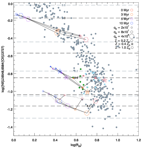
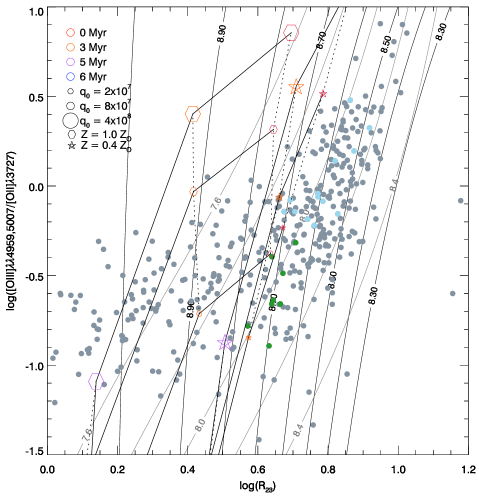
Figure 8: Left: log R₂₃ vs. log [N ii]/[O ii]. We show lines of constant metallicity based on the N2O2 calibrations of Kewley & Dopita (2002, black dashes) and Bresolin (2007, grey dashes). Right: log R₂₃ vs. log [O iii]/[O ii]. We show lines of constant metallicity, based on the upper (black lines) and lower (grey) branches of the R₂₃ calibration of McGaugh (1991). In both panels the grey dots show the same sample of H ii regions plotted in previous figures. Cyan dots represent H ii regions from our NGC 4625 sample for which [O iii]/H$\beta>0.25$, whilst green dots represent those with [O iii]/H$\beta<0.25$. We have also plotted itera nebular models using the same symbols as in Fig. 6.

The left-hand panel of Fig. 8 gives us two major insights. Firstly, it confirms our earlier finding (§4.2.2) that the line emission properties of ageing H ii regions appear to replicate those of the H ii regions in our sample which were found to lie off the main ionisation sequence in the BPT diagnostic diagram (green dots). Secondly, it shows how an ageing population of H ii regions might affect the determination of the chemical abundances. The itera models suggest that as an H ii region ages, its R₂₃ value rapidly decreases, resulting in a shift almost parallel to the lines of constant metallicity (determined using the N2O2 diagnostic). The [N ii]/[O ii] ratio also changes, simulating a variation in the inferred metallicity. Therefore, the models give us an indication of how reliable the metallicity indicators become for an ageing H ii region population. A spread of ages of, say, between 3 and 6 Myr, as suggested by Fig. 7 for NGC 4625, could result in an uncertainty in the abundance measurement of roughly $\sim 0.15$ dex, based on the N2O2 diagnostic.

The right-hand panel of Fig. 8 helps us to identify how robust the R₂₃ indicator may be against such an ageing H ii region population. For a metallicity of 0.4 $Z_{\odot}$  the H ii regions appear to evolve almost parallel to the lines of constant metallicity, although there may be some divergence with the lower branch calibration for the oldest models. However, for the 1 $Z_{\odot}$ metallicity case the H ii region evolution appears to be problematic for the models, since large changes in the measured abundance, of the order $\sim$0.25 dex, appear to occur, together with discrepancies for models of the same age but lower ionisation parameters. This suggests that for an ageing population of H ii regions with a spread of ionisation parameters the R₂₃ indicator could represent an inaccurate measure of the oxygen abundance.

5 Discussion

5.1 Breaks in Abundance Gradients

In §3.2 we showed that the strong line abundance indicators used in this study gave qualitatively similar results. All showed a discontinuity in the abundance gradient at a galactocentric distance between 0.7 and 1.1 R₂₅, and a shallower gradient in the outer disc.

While the abundance solution provided by the use of the R₂₃ indicator remains somewhat dubious, due to the uncertainty in the choice between upper and lower branch calibration, the N2 and N2O2 abundance diagnostics are monotonic with abundance and are unlikely to produce false discontinuities or gradient changes. In addition, Bresolin et al. (2009a) tested the reliability of N2O2 to measure relative abundances in both the inner and outer disc of M83.

In both NGC 4625 (this work) and in M83 (Bresolin et al. 2009a) we found a discontinuity in the abundance gradient, with a shallower slope beyond R₂₅. Goddard et al. (2010) also found similar radial UV and H$\alpha$  profiles in the two galaxies. The FUV profile is smooth over the transition between inner and outer disc, becoming shallower beyond R₂₅. Conversely, the H$\alpha$ profiles show a sharp truncation at R₂₅, in correspondence with the edge of the star forming disc. The origin of these effects lies possibly in the differing star formation properties between inner and outer parts of the discs we have analyzed. The extremely low H$\alpha$ emission in the extended discs indicates a very low star formation rate (Gil de Paz et al., 2005; Goddard et al., 2010). The lack of massive stars results in a smaller chemical enrichment from supernova events, which would eventually lead to the oxygen abundance discontinuity observed between the inner and outer discs. G07 have argued that both a low-level, but continuous, star formation activity and an episodic one could be invoked to explain the fact that the oxygen abundances are low, but not extremely so, in the extended discs of spirals (see also Bresolin et al. 2009a). Bresolin et al. (2009a) have remarked on the similarity between XUV discs and low-surface brightness galaxies in terms of chemical abundances and enrichment. They also pointed out that gravitational interactions with companion galaxies could generate, via gas stripping, peculiarities in the abundance gradients, such as those observed in the outer disc of M83, which has likely interacted with NGC 5253 around 1 Gyr ago. The situation appears to be similar in the case of NGC 4625, which has been in interaction with its companion NGC 4618 and, possibly, a fainter galaxy (Gil de Paz et al. 2005). Perhaps these interactions play an important role both in the activation of the star formation in the extended discs, and in the generation of the abundance breaks and/or flattened gradients.

5.2 H II Region populations in XUV discs

We found a significant number of H ii regions in NGC 4625 that appear to depart from the main ionisation sequence established by studies of bright, inner disc ionized nebulae. A similar behaviour is detected (Fig. 2) for a small fraction of H ii regions in other galaxies. The most likely reasons for this anomaly have been identified in stochasticity or the effects of an ageing H ii region population. Since the outer disc H ii regions contain at most only a few O-type stars, the source of ionizing flux is subject to stochastic variations (Gil de Paz et al., 2005; Thilker et al., 2005; Goddard et al., 2010). By using measurements from Goddard et al. (2010), in combination with published photoionisation models, we also found that an ageing H ii region population might equally be responsible for the spread we observe in the BPT diagnostic diagram. These two effects are indistinguishable, since an evolving H ii region loses first the most massive stars, which are also those that are most affected by stochastic variations.

We examined the possibility that geometry or a non-standard N/O ratio might explain the emission line properties of the deviant H ii regions. However, we concluded that these effects are unlikely to produce the observed trends, and both age and stochastic arguments appear to be more robust. It was never our intent to produce a full description of these effects, but only to highlight the fact that outer disc H ii regions are significantly different from their inner disc counterparts, and this difference has not been fully investigated yet. In the future it will be important to investigate the presence of H ii regions in other galaxies with emission line properties similar to what we found in NGC 4625, and carry out new comparisons to models generated with a stochastically populated IMF.

6 Conclusions

In this study we have analysed the spectra of 34 H ii regions at a range of galactocentric radii in the XUV disc galaxy NGC 4625. Below we summarise our main findings:

1.

Strong line abundance indicators consistently show a shallower abundance gradient in the outer disc compared to the inner disc. This is accompanied by a discontinuity in the abundance gradient that occurs in proximity of the optical edge of the galaxy. These trends are very similar to those seen in M83.

2.

The three T_e-based abundances in the outer disc predict a metallicity of 12 + log(O/H) $\simeq 7.96\,\pm\,^{0.22}_{0.31}$ ($\sim 0.2$ $Z_{\odot}$) in the outer disc.

3.

We identified a subset of outer disc H ii regions which do not conform to the ionisation sequence defined by the bright inner disc H ii regions in the [O iii]/H$\beta$ vs. [N ii]/H$\alpha$ diagnostic diagram. These objects do not appear to display any unique properties in terms of position within the XUV disc or ionising flux.

4.

Stochastic variations in the high-mass end of the embedded stellar population or an ageing H ii region population seem to be the most likely effects capable of producing the observed emission line properties. However, it has not been possible to distinguish between these two effects.

5.

The strong line abundance indicators used in this paper appear to be less reliable if the H ii region population is ageing, even over the short 10 Myr timescale of the ionising stars. This effect could be as much as $\sim$ 0.15 dex for the N2O2 indicator, and even more for R₂₃.

We hope future studies of outer disc H ii regions will be able to further probe this regime of stochastically determined ionisation sources. It is only through the continued study of the abundance gradients in a variety of XUV discs that we may hope to better understand the connection between star formation and chemical enrichment of the interstellar medium in these low gas density environments.

FB gratefully acknowledges the support from the National Science Foundation grant AST-0707911.

References

- Asplund et al. (2009) Asplund M., Grevesse N., Sauval A. J., Scott P., 2009, ARAA, 47, 481
- Baldwin et al. (1981) Baldwin J. A., Phillips M. M., Terlevich R., 1981, PASP, 93, 5
- Bianchi et al. (2003) Bianchi L., Madore B., Thilker D., et al., 2003, Bulletin of the American Astronomical Society, 35, 1354
- Bresolin et al. (2009a) Bresolin F., Ryan-Weber E., Kennicutt R. C., Goddard Q., 2009a, ApJ, 695, 580
- Bresolin et al. (2009b) Bresolin F., Gieren W., Kudritzki R., Pietrzyński G., Urbaneja M. A., Carraro G., 2009b, ApJ, 700, 309
- Bresolin (2008) Bresolin F., 2008, in The Metal-Rich Universe, G. Israelian & G. Meynet ed. (Cambridge University Press, Cambridge), p. 155
- Bresolin (2007) Bresolin F., 2007, ApJ, 656, 186
- Bresolin et al. (2005) Bresolin F., Schaerer D., González Delgado R. M., Stasińska G., 2005, A&A, 441, 981
- Bresolin & Kennicutt (2002) Bresolin F., Kennicutt Jr. R. C., 2002, ApJ, 572, 838
- Bresolin et al. (1999) Bresolin F., Kennicutt Jr. R. C., Garnett D. R., 1999, ApJ, 510, 104
- Bush et al. (2008) Bush S. J., Cox T. J., Hernquist L., Thilker D., Younger J. D., 2008, ApJL, 683, L13
- Bush & Wilcots (2004) Bush S. J., Wilcots E. M., 2004, AJ, 128, 2789
- Christlein & Zaritsky (2008) Christlein D., Zaritsky D., 2008, ApJ, 680, 1053
- Cuillandre et al. (2001) Cuillandre J., Lequeux J., Allen R. J., Mellier Y., Bertin E., 2001, ApJ, 554, 190
- Davidge (2007) Davidge T. J., 2007, ApJ, 664, 820
- de Vaucouleurs et al. (1991) de Vaucouleurs G., de Vaucouleurs A., Corwin Jr. H. G., Buta R. J., Paturel G., Fouque P., 1991, Third Reference Catalogue of Bright Galaxies. Springer-Verlag
- Dong et al. (2008) Dong H., Calzetti D., Regan M., Thilker D., Bianchi L., Meurer G. R., Walter F., 2008, AJ, 136, 479
- Dopita et al. (2000) Dopita M. A., Kewley L. J., Heisler C. A., Sutherland R. S., 2000, ApJ, 542, 224
- Elmegreen & Hunter (2006) Elmegreen B. G., Hunter D. A., 2006, ApJ, 636, 712
- Ercolano et al. (2007) Ercolano B., Bastian N., Stasińska G., 2007, MNRAS, 379, 945
- Ferguson et al. (1998a) Ferguson A. M. N., Gallagher J. S., Wyse R. F. G., 1998a, AJ, 116, 673
- Ferguson et al. (1998b) Ferguson A. M. N., Wyse R. F. G., Gallagher J. S., Hunter D. A., 1998b, ApJL, 506, L19
- Gil de Paz et al. (2008) Gil de Paz A., Thilker D. A., Bianchi L., et al., 2008, in J. G. Funes & E. M. Corsini ed., Astronomical Society of the Pacific Conference Series Vol. 396, Extended UV (XUV) Emission in Nearby Galaxy Disks. p. 197
- Gil de Paz et al. (2007) Gil de Paz A., Madore B. F., Boissier S., et al., 2007, ApJ, 661, 115
- Gil de Paz et al. (2005) Gil de Paz A., Madore B. F., Boissier S., et al., 2005, ApJL, 627, L29
- Goddard et al. (2010) Goddard Q. E., Kennicutt R. C., Ryan-Weber E. V., 2010, MNRAS, p. 644
- Groves & Allen (2010) Groves B. A., Allen M. G., 2010, New Astronomy, 15, 614
- Kashikawa et al. (2002) Kashikawa N., Aoki K., Asai R., et al., 2002, PASJ, 54, 819
- Kennicutt et al. (2003) Kennicutt Jr. R. C., Armus L., Bendo G., et al., 2003, PASP, 115, 928
- Kennicutt et al. (2000) Kennicutt Jr. R. C., Bresolin F., French H., Martin P., 2000, ApJ, 537, 589
- Kennicutt (1998) Kennicutt Jr. R. C., 1998, ARAA, 36, 189
- Kennicutt & Garnett (1996) Kennicutt Jr. R. C., Garnett D. R., 1996, ApJ, 456, 504
- Kennicutt (1989) Kennicutt Jr. R. C., 1989, ApJ, 344, 685
- Kewley & Ellison (2008) Kewley L. J., Ellison S. L., 2008, ApJ, 681, 1183
- Kewley et al. (2006) Kewley L. J., Groves B., Kauffmann G., Heckman T., 2006, MNRAS, 372, 961
- Kewley & Dopita (2002) Kewley L. J., Dopita M. A., 2002, ApJS, 142, 35
- Kobulnicky et al. (1999) Kobulnicky H. A., Kennicutt Jr. R. C., Pizagno J. L., 1999, ApJ, 514, 544
- Leitherer et al. (1999) Leitherer C., Schaerer D., Goldader J. D., Delgado R. M. G., Robert C., Kune D. F., de Mello D. F., Devost D., Heckman T. M., 1999, ApJS, 123, 3
- Lelièvre & Roy (2000) Lelièvre M., Roy J.-R., 2000, AJ, 120, 1306
- Levesque et al. (2010) Levesque E. M., Kewley L. J., Larson K. L., 2010, AJ, 139, 712
- Martin & GALEX Science Team (2003) Martin C., GALEX Science Team 2003, in Bulletin of the American Astronomical Society Vol. 35, The Galaxy Evolution Explorer (GALEX). p. 1363
- Martin & Kennicutt (2001) Martin C. L., Kennicutt Jr. R. C., 2001, ApJ, 555, 301
- Martins et al. (2005) Martins F., Schaerer D., Hillier D. J., 2005, A&A, 436, 1049
- McCall et al. (1985) McCall M. L., Rybski P. M., Shields G. A., 1985, ApJS, 57, 1
- McGaugh (1991) McGaugh S. S., 1991, ApJ, 380, 140
- Oey & Shields (2000) Oey M. S., Shields J. C., 2000, ApJ, 539, 687
- Osterbrock (1989) Osterbrock D. E., 1989, Astrophysics of gaseous nebulae and active galactic nuclei. University Science Books
- Pérez-Montero & Díaz (2005) Pérez-Montero E., Díaz A. I., 2005, MNRAS, 361, 1063
- Pettini & Pagel (2004) Pettini M., Pagel B. E. J., 2004, MNRAS, 348, L59
- Pflamm-Altenburg & Kroupa (2008) Pflamm-Altenburg J., Kroupa P., 2008, Nature, 455, 641
- Pilyugin & Thuan (2005) Pilyugin, L. S. & Thuan, T. X. 2005, ApJ, 631, 231
- Rosales-Ortega et al. (2010) Rosales-Ortega F. F., Kennicutt R. C., Sánchez S. F., Díaz A. I., Pasquali A., Johnson B. D., Hao C. N., 2010, MNRAS, p. 461
- Thilker et al. (2007) Thilker D. A., Bianchi L., Meurer G., et al., 2007, ApJS, 173, 538
- Thilker et al. (2005) Thilker D. A., Bianchi L., Boissier S., et al., 2005, ApJL, 619, L79
- van Zee et al. (1998) van Zee L., Salzer J. J., Haynes M. P., O’Donoghue A. A., Balonek T. J., 1998, AJ, 116, 2805
- Veilleux & Osterbrock (1987) Veilleux S., Osterbrock D. E., 1987, ApJS, 63, 295
- Zaritsky & Christlein (2007) Zaritsky D., Christlein D., 2007, AJ, 134, 135