A physical interpretation of the cubic map coefficients describing the electron cloud evolution

Abstract

The Electron Cloud (ecloud), an undesirable physical phenomena in the accelerators, develops quickly as photons striking the vacuum chamberwall knock out electrons that are then accelerated by the beam, gain energy, and strike the chamber again, producing more electrons. The interaction between the electron cloud and a beam leads to the electron cloud effects such as single- and multi-bunch instability, tune shift, increase of pressure and particularly can limit the ability of recently build or planned accelerators to reach their design parameters. We report a principal results about the analytical study to understanding a such dynamics of electrons.

I Introduction

The generation of a quasi-stationary electron cloud inside the beam pipe through beam-induced multipacting has become an area of intensive study. The analysis performed so far was based on very heavy computer simulations (ECLOUD zim ) taking into account photoelectron production, secondary electron emission, electron dynamics, and space charge effects providing a very detailed description of the electron cloud evolution.

In iriso1 has been shown that, for the typical parameters of Relativistic Heavy Ion Collider (RHIC), the evolution of the electron cloud density can be followed from bunch to bunch introducing a ”cubic map” of the form:

$$n_{m+1}\,=\,\alpha\,n_{m}+\beta\,{n_{m}}^{2}+\gamma\,{n_{m}}^{3}$$ (1)

where $n_{m}$ is the average electron cloud density after $m$-th passage of bunch, $n_{m+1}$ is the one after $(m+1)$-th passage. The coefficients $\alpha$, $\beta$, $\gamma$ are the parameters extrapolated from simulations, and are functions of the beam parameters and of the beam pipe features. The average longitudinal electron density as function of time grows exponentially until the space charge due to the electrons themselves produces a saturation level. Once the saturation level is reached the average electron density does not change significantly. The final decay corresponds to the succession of the empty bunches.

A such map approach has been proved, by numerical simulations, reliable also for Large Hadron Collider (LHC) demma . The most important outcomes of map formalism for LHC (and generally for any accelerator) are summarizable as follows. In Fig. 1 one can see that the bunch-to-bunch evolution contains enough information about the build-up or the decay time, although the details of the line electron density oscillation between two bunches are lost.

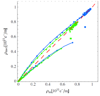
Figure 1: Time evolution of the electron density (green line) computed with ECLOUD. The black dots mark the average electron density between two consecutive bunches.

Fig. 2 shows the behavior of the average electron density $n_{m+1}$, after the passage of $(m+1)$-th bunch, as function of the average electron density as $n_{m}$ for different bunch intensities.

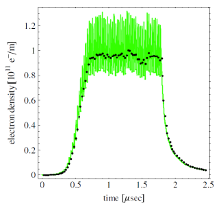
Figure 2: Average longitudinal electron density after the passage of bunch as a function of longitudinal electron density $n_{m+1}$ before the passage of $m$-th bunch, for different bunch intensities (green $N_{b}\,=\,8*10^{10}$, blue $N_{b}\,=\,16*10^{10}$). The lines correspond to cubic fits applied to the average bunch to bunch points. The red line corresponds to the identity map $n_{m+1}\,=\,n_{m}$. Points above this line describe the initial growth and saturation of the bunch-to-bunch evolution of the line electron density, those below describe the decay. The black line represents the cubic fit to the points corresponding to the first empty bunches.

The points in Fig. 2 show the average electron cloud density between two bunches using results from ECLOUD, the lines are cubic fits to these points. The physical dynamics of electron cloud is explained as follows: starting with a small initial linear electron density, after some bunches the density takes off and reaches the corresponding saturation line ($n_{m+1}\,=\,n_{m}$, red line) where the space charge effects due to the electrons in the cloud itself take place. In this situation, all the points (corresponding to the passage of full bunches) are in the same spot. The justification of the three terms in eq. (1) is explained as a consequence of the linear growth (this term has to be larger than unity in case of electron cloud formation), a parabolic decay due to space charge effects (this term has to be negative to give concavity to the curve $n_{m+1}$ vs $n_{m}$), and a cubic term corresponding to perturbations. Neglecting the point corresponding to the electron cloud density after the first empty bunch, the longitudinal electron density follows a similar decay independently of the initial value of the saturated line electron density. The points corresponding to the first empty bunches coming from different saturation values lie on a general curve (black curve in Fig. 2). Thus the electron density build up for a given bunch intensity is determined by a cubic form, while decay is described by two different cubic forms, one corresponding to the first empty bunch, and a second to the rest.

Even though the behavior of the map coefficients from simulations has been compared with the experiments always this is not well understood and the determination of their values is purely empirical. An analytical expression for coefficient $\alpha$ (linear coefficient) in the case of drift space has been found by understanding the dynamics that governs weak cloud behavior iriso1 .

Let us consider $N_{el,m}$ quasi-stationary electrons gaussian-like distributed in the transverse cross-section of the beam pipe. The $(m+1)$-th bunch accelerates the $N_{el,m}$ electrons initially at rest to an energy $\mathcal{E}_{g}$. After the first wall collision two new jets are created: the backscattered one with energy $\mathcal{E}_{g}$ and proportional to $\delta_{r}(\mathcal{E}_{g})$, and the ”true secondaries” (with energy $\mathcal{E}_{0}\,\sim\,5\,eV$) proportional to $\delta_{t}(\mathcal{E}_{0})$. The functions $\delta$’s (or $SEY$: Secondary emission yield) give the ratio of emitted secondary electrons per incident electron. The sum of all these jets becomes the number of surviving electrons $N_{el,m+1}$ (see section III), and we have

$$\alpha\,=\,\frac{N_{el,m+1}}{N_{el,m}}$$ (2)

In this paper we derive, by assuming the previous theoretical expression for linear coefficient ($\alpha$) iriso1 , a simple approximate formula for the quadratic coefficient ($\beta$), which determines the saturation of the cloud due to space charge, in the electron cloud density map, under the assumptions of round chambers and free-field motion of the electrons in the cloud. The coefficient depends on the bunch parameters, and can be simply deduced from ecloud simulation codes modelling the involved physics in full detail. Results are compared with simulations for a wide range of parameters governing the evolution of the electron cloud.

In the section II we calculate the electronic density of saturation by imposing a gaussian-like distribution for the space charge and requiring the presence of energy barrier near to wall of chamber. In the section III we report the calculus of linear coefficient and we compute the calculus of quadratic term. Once calculated saturation we pass to estimate theoretically the coefficient $\beta$. We conclude (section IV) with the comparison with respect to outcomes of numerical simulations obtained using ECLOUD zim . In the table 1 we report all parameters used for the the calculations.

Parameter Quantity Unit Value Beam pipe radius $b$ m $.045$ Beam size $a$ m $.002$ Bunch spacing $s_{b}$ m $1.2$ Bunch length $h$ m $.013$ Energy for $\delta_{max}$ $\mathcal{E}_{0,max}$ eV $300$ - $\mathcal{E}_{r}$ eV $60$ Particles per bunch $N_{b}$ $10^{10}$ $4\,\div\,9$ SEY (max) $\delta_{max}$ - $1.7$ SEY ($\mathcal{E}\rightarrow 0$) $\delta_{0}$ - $.7$ SEY ($\mathcal{E}\rightarrow\infty$) $\delta_{\infty}$ - $.15$ - $\zeta$ - 1.83

Table 1: Input parameters for analytical estimate and ECLOUD simulations.

II Steady-state: Electronic density of Saturation

In the chamber we have two groups of electrons belonging to cloud: primary photo-electrons generated by the synchrotron radiation photons and secondary electrons generated by the beam induced multi-pactoring. Electrons in the first group generated at the beam pipe all with the radius $b$ interact with the parent bunch and accelerated (by a short bunch) to the velocity $v/c\,=\,2\bar{N}_{b}r_{e}/b$, where $r_{e}$ is the classical electron radius and $\bar{N}_{b}$ is the efficacy value of bunch population. Since we are in presence of trains of finite length beams to consider a similar analysis to costing hypothesis it should replace the value of bunch population with its spatial or temporal average. In fact we have

$$\bar{N}_{b}\,=\,\frac{h}{h+s_{b}}N_{b}$$ (3)

where $s_{b}$ is the bunch spacing and $h$ is the length of bunch. Electrons in the second group, generally, miss the parent bunch and move from the beam pipe wall with the velocity $v/c\,=\,\sqrt{2\mathcal{E}_{0}/mc^{2}}$ until the next bunch arrives. The velocity is defined by the average energy $\mathcal{E}_{0}$ of the secondary electrons and, at high $\bar{N}_{b}$, is smaller than velocity of the first group. The process of the cloud formation depends, respectively, on two parameters:

$$k\,=\,\frac{2\bar{N}_{b}r_{e}h}{b^{2}}$$ (4)

$$\xi\,=\,\frac{h}{b}\sqrt{\frac{2\mathcal{E}_{0}}{mc^{2}}}$$ (5)

These parameters are the distance (in units of $b$) passed by electrons of each group before the next bunch arrives. At low currents, $k\,<<\,1$, electron interact with many bunches before it reaches the opposite wall. In the opposite extreme case, $k\,>\,2$, all electrons go wall to wall in one bunch spacing. The transition to the second regime can be expected , therefore, $k\,\sim\,1$ where the cloud is quite different than it is at low currents. For $k\,>\,1$, secondary electrons are confined within the layer $\xi\,<\,r/b\,<\,1$ at he wall and are wiped out of the region $0\,<\,r/b\,<\,\xi$ close to the beam by each passing bunch. This makes the range of parameters ($k\,>\,1$ and $2-k\,<\,\xi\,<1$) quite desirable to suppress the adverse effects of the e-cloud on the beam dynamics eifets .

The condition of neutrality implies that secondary electrons remain in the cloud for a time long enough to affect the secondary electrons generated by the following bunches. In other words, the condition of neutrality and the quasi-steady equilibrium distribution of the electron cloud are justified only for small $k$. It is not the case at the high currents. In this case, all primary photo-electrons disappear just in one pass. The secondary electrons are produced with low energy $\mathcal{E}_{0}$ and are locked up at the wall. The density of the secondary electrons grows until the space-charge potential of the secondary electrons is lower than $\mathcal{E}_{0}$. The saturation condition can be obtained by requiring that the potential barrier is greater than electron energy in the point $r/b\,=\,1-\xi$

$$-e\,V(1-\xi)\,\sim\,\mathcal{E}_{0}$$ (6)

where $V$ is the electric potential generated by the bunch and electron cloud and $-e$ is the electron charge. Here it needs to calculate the electric potential by assuming some model for the electronic density.

Our system is composed by a chamber with radius $b$, a bunch with radius $a$ and length $h$, an electron cloud with density $\rho$. Let us consider a electron cylindric distribution with a radial gaussian density centered in $r_{0}$ as follows

$$\rho(r)\,=\,\rho_{0}e^{-\frac{(r-r_{0})^{2}}{2\sigma^{2}}}$$ (7)

where $\rho_{0}$ is fixed by the condition

$$2\pi h\int_{a}^{b}\rho(r)rdr\,=\,-N_{el}\,e$$ (8)

where $N_{el}$ is the total number of electrons in the volume $\pi h(b^{2}-a^{2})$. The electric field in the chamber is

$$\vec{E}\,=\, \biggl{\{}\frac{\bar{N}_{b}\,e}{2\pi\epsilon_{0}h}\frac{1}{r}-\frac{N_{el}\,e}{2\pi\epsilon_{0}h}\frac{1}{\int_{a}^{b}e^{-\frac{(y-r_{0})^{2}}{2\sigma^{2}}}ydy}\times$$ (9)

$$\times\frac{\int_{a}^{r}e^{-\frac{(y-r_{0})^{2}}{2\sigma^{2}}}ydy}{r}\biggr{\}}\hat{r}$$

The electric potential $V(r)$ defined by the condition $V(b)\,=\,0$ is

$$V(r)\,= \int_{r}^{b}\vec{E}\cdot d\vec{l}\,=\,$$ (10)

$$-\frac{\bar{N}_{b}\,e}{2\pi\epsilon_{0}h}\ln\frac{r}{b}-\frac{N_{el}\,e}{2\pi\epsilon_{0}h}\frac{\int_{r}^{b}\,\frac{\int_{a}^{y}\,e^{-\frac{(z-r_{0})^{2}}{2\sigma^{2}}}z\,dz}{y}dy}{\int_{a}^{b}\,e^{-\frac{(y-r_{0})^{2}}{2\sigma^{2}}}y\,dy}\,=$$

$$-\frac{\bar{N}_{b}\,e}{2\pi\epsilon_{0}h}\ln x-\frac{N_{el}\,e}{2\pi\epsilon_{0}h}\frac{G(x)}{F(1)}\,=$$

$$-V_{0}\biggl{[}g\ln x+\frac{G(x)}{F(1)}\biggr{]}$$

where $F(x)\,=\,\int_{\tilde{a}}^{x}\,e^{-\frac{(\tilde{y}-\tilde{r}_{0})^{2}}{2\tilde{\sigma}^{2}}}y\,dy$, $G(x)\,=\,\int_{x}^{1}\,\frac{F(y)}{y}dy$, $g\,=\,\bar{N}_{b}/N_{el}$, $V_{0}\,=\,\frac{N_{el}\,e}{2\pi\epsilon_{0}h}$ and $x\,=\,r/b$, $\tilde{a}\,=\,a/b$, $\tilde{r}_{0}\,=\,r_{0}/b$, $\tilde{\sigma}\,=\,\sigma/b$. We note that in the case $\sigma\,>>\,b$ (or $\tilde{\sigma}\,>>\,1$) and $r_{0}\,=\,0$ we reobtain the uniform electron cloud and with $a\,\rightarrow\,0$ we must neglect the radial dimension of bunch with respect to one of electron cloud. In fact in this case for eq. (10) we would have

$$V_{ud}(r)\,=\,-V_{0}\biggl{[}g\ln x+\frac{1-x^{2}}{2}\biggr{]}$$ (11)

Obviously the potentials depend on $g$, the ratio of the densities of the beam and of the cloud averaged over the beam pipe cross-section. In Fig. 3 we report the spatial behavior of two potentials. The potential (11) has minimum at $r\,=\,r_{m}\,=\,b\sqrt{g}$ and is monotonic for $g\,>\,1$ within the beam pipe. For $g\,<\,1$ it has minimum at the distance $r_{m}\,<\,b$, and the condition $g\,=\,1$ defines the maximum density. this is the well known condition of the neutrality. The condition formulated in this form is, actually, independent of the form of distribution. Similar behavior is found also for the gaussian distribution density and is compared with respect to previous one (Fig. 3).

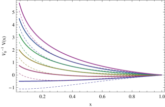
Figure 3: Plot of $V_{0}^{-1}V(x)$, (10) and (11)), in the case of uniform (solid lines) and gaussian (dashed lines) electronic distribution for $g\,=\,0\,\div\,2$, $\tilde{a}\,=\,.04$, $\tilde{r}_{0}\,=\,0$, $\tilde{\sigma}\,=\,.3$.

By imposing the condition eq. (6) we find the critical number (saturation condition) of electrons in the chamber

$$N_{el,sat}\,=\,\frac{2\pi\epsilon_{0}hF(1)\mathcal{E}_{0}}{e^{2}G(1-\xi)}-\frac{F(1)\ln(1-\xi)}{G(1-\xi)}\bar{N}_{b}$$ (12)

while the average density of saturation is found by assuming that electrons are confined in a cylindrical shell with inner radius equal to $a$ and external radius to $r_{0}+p\,\sigma$ where $p$ is a free parameter. So

$$n_{sat}\,=\,\frac{N_{el,sat}}{\pi hb^{2}[(\tilde{r}_{0}+p\,\tilde{\sigma})^{2}-\tilde{a}^{2}]}$$ (13)

where $p$ is a free parameter. In the case of uniform distribution of electron cloud with a similar mathematical passages we find the density of saturation

$$\bar{n}_{sat}\,=\,\frac{\bar{N}_{el,sat}}{\pi hb^{2}[1-\tilde{a}^{2}]}$$ (14)

In the Fig. 4 we show the behavior of density of saturation (13) and (14). It is obvious in the case of a gaussian distribution of cloud we get a estimate of density saturation greater than that of uniform distribution. In fact, the same number of electrons occupies a smaller volume (due to the Gaussian distribution).

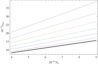
Figure 4: Plot of electronic densities of saturation $n_{sat}$ vs $N_{b}$, (13) and (14)), in the case of uniform (solid line) and gaussian (dashed lines) electronic distribution for $\tilde{a}\,=\,.04$, $\tilde{r}_{0}\,=\,0$, $\tilde{\sigma}\,=\,.3$ and $p\,=\,2\,\div\,3$

III Analytical Determination of Coefficients

To compute the linear term we can assume that all the $N_{el,m}$ electrons, distributed in the transverse cross section of the beam pipe, gain an energy $\mathcal{E}_{g}$ during the passage of the bunch $m$. After the bunch passage, electrons are accelerated towards the chamber wall and have their first wall collision when two new jets are created: one with energy $\mathcal{E}_{g}$ and $N_{m}\delta_{r}$ electrons, corresponding to backscattered electrons; the second with low energy and $N_{m}\delta_{t}$ electrons, corresponding to the true secondaries. Before $(m+1)$-th bunch arrives, these two jets perform several wall collisions, which in turn create more jets. The contribution of all these jets becomes the number of surviving electrons, $N_{m+1}$. The reflected electrons travel across the beam pipe with energy $\mathcal{E}_{g}$ and perform a number of collisions with the chamber wall, between two consecutive bunches, that is:

$$s\,=\,\frac{t_{sb}-t_{f}(\mathcal{E}_{g})}{t_{f}(\mathcal{E}_{g})},$$ (15)

where $t_{sb}$ is the time of bunch spacing,

$$t_{f}(\mathcal{E}_{g})\,=\,\frac{4b}{\pi\sqrt{2\mathcal{E}_{g}/m_{e}}}$$ (16)

is the average flight time and $\mathcal{E}_{g}$ is the energy of electrons accelerated by bunch

$$\mathcal{E}_{g}\,=\,m_{e}c^{2}\frac{r_{e}N_{b}}{\sqrt{2\pi}h}\biggl{[}\log\biggl{(}\frac{b}{1.05a}\biggr{)}-\frac{1}{2}\biggr{]}$$ (17)

Hence, the total number of reflected, high energy electrons at the passage of $m+1$-th bunch is:

$$N_{el|ref}\,=\,N_{el,m}{\delta_{r}}^{s}$$ (18)

The true secondaries electrons produced after the first wall collision gives rise to a low energy jet ($\mathcal{E}_{0}$). For this jet there is no distinction for the true secondaries and reflected, since all are produced with the same energy. After the $i-$th wall collision the number of surviving electrons is:

$$N_{el|tot}\,=\,N_{el,m}\,\delta_{t}\,{\delta_{r}}^{i-1}\,{\delta_{tot}}^{k_{i}}$$ (19)

where $\delta_{tot}\,=\,\delta_{r}(\mathcal{E}_{0})+\delta_{t}(\mathcal{E}_{0})$ and

$$k_{i}\,=\,\frac{t_{sb}-it_{f}(\mathcal{E}_{0})}{t_{f}(\mathcal{E}_{0})},$$ (20)

is the number of collisions after the $i-$th collision. The low energy electrons at the passage of $m+1$-th bunch is :

$$N_{el|s}\,=\,N_{el,m}\delta_{t}\,\sum_{i=1}^{s}{\delta_{r}}^{i+1}{\delta_{tot}}^{k_{i}}$$ (21)

Finally the total number of survival electrons at $m+1$-th bunch passage is obtained taking into account both the high and low energy contributions:

$$N_{el,m+1}\,=\,N_{el,m}\biggl{[}{\delta_{r}}^{s}+\delta_{t}\sum_{i=1}^{s}{\delta_{r}}^{i+1}{\delta_{tot}}^{k_{i}}\biggr{]}$$ (22)

and the linear term (2) can be written in the form:

$$\alpha\,=\,\frac{N_{el,m+1}}{N_{el,m}}\,=\,{\delta_{r}}^{s}+\delta_{t}{\delta_{tot}}^{\eta}\,\frac{{\delta_{tot}}^{s\eta}-{\delta_{r}}^{s}}{{\delta_{tot}}^{\eta}-{\delta_{r}}^{s}}$$ (23)

where $\eta\,=\,\sqrt{\mathcal{E}_{0}/\mathcal{E}_{g}}$. The expressions of $\delta$’s used are

$$\left\{\begin{array}[]{ll}\delta_{r}(\mathcal{E})\,=\,\delta_{\infty}+(\delta_{0}-\delta_{\infty})e^{-\frac{\mathcal{E}}{\mathcal{E}_{r}}}\\ \\ \delta_{t}(\mathcal{E})\,=\,\zeta\,\delta_{max}\frac{\mathcal{E}}{\mathcal{E}_{0,max}}\frac{1}{\zeta-1+\frac{\mathcal{E}^{\zeta}}{{\mathcal{E}_{0,max}}^{\zeta}}}\end{array}\right.$$ (27)

where $\delta_{\infty}$, $\delta_{0}$, $\mathcal{E}_{r}$, $\zeta$, $\delta_{max}$, $\mathcal{E}_{0,max}$ are the parameters of models and their values are shown in Table 1. The coefficient $\beta$ can be found by imposing the saturation condition of map (1):

$$n_{sat}\,=\,\alpha\,n_{sat}+\beta\,{n_{sat}}^{2}\,\,\,\,\rightarrow\,\,\,\,\beta\,=\,\frac{1-\alpha}{n_{sat}}$$ (28)

and the map (1) becomes

$$n_{m+1}\,=\,\alpha\,n_{m}+\frac{1-\alpha}{n_{sat}}\,{n_{m}}^{2}$$ (29)

In Fig. (5), (6) we show the trends of the coefficient (28) as a function of $\delta_{max}$ for various values of bunch population and viceversa.

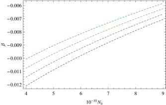
Figure 5: Analytical prediction of coefficient $\beta$ (28) for values $\delta_{max}\,=\,1.4\div 2$ and $p\,=\,2$.

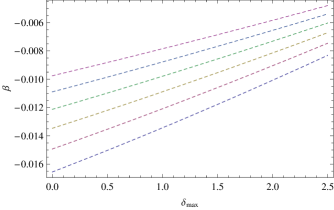
Figure 6: Analytical prediction of coefficient $\beta$ (28) for values $N_{b}\,=\,(4\div 9)*10^{10}$ and $p\,=\,2$.

IV Conclusions

In Figs. (7) and (8) we report the analytical behaviors and the outcomes of simulations (ECLOUD code) of coefficients $\alpha$ and $\beta$ for values in table 1. It is important to note about the quadratic coefficient we had a good agreement with simulations because in our theoretical treatment we have a degree of freedom due to the choice of charge distribution in the chamber. By requiring the condition of saturation it needs to choose an average density that can be as realistic as possible. A similar discourse was not possible for the linear term because we started from the result of Iriso & Peggs (iriso2 ) and then we built the working hypothesis for the determination of $\beta$. This specification allows us to evaluate the apparent discrepancy between the linear and quadratic coefficient with respect to their results from ECLOUD code.

The radial profile of electric density $n(r)$, from (7), is

$$n(r)\,=\,\frac{\rho(r)}{-e}\,=\,\frac{N_{el,sat}}{2\pi hb^{2}}\frac{e^{-\frac{(x-\tilde{r}_{0})^{2}}{2\tilde{\sigma}^{2}}}}{F(1)}$$ (30)

and one of energy barrier which opposes the electron coming from the wall, from (10), is

$$\mathcal{E}(r)\,=\,-e\,V(r)\,=\,e\,V_{0}\biggl{[}g\ln x+\frac{G(x)}{F(1)}\biggr{]}$$ (31)

and we report in Fig. (9) their behavior. It notes how the peak of the energy barrier corresponds to the maximum concentration of electrons around the bunch charge. As soon as the density of electrons tends to zero near the wall of chamber also energy barrier tends to zero.

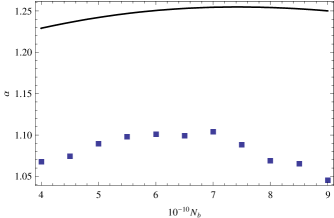
Figure 7: Comparison between the analytical prediction (solid line) of $\alpha$ (Eq. (23)) and the simulation (points) by ECLOUD code.

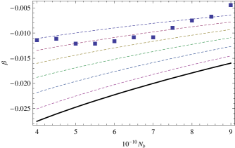
Figure 8: Comparison of the quadratic coefficient $\beta$ (Eq. (28)) derived using ECLOUD simulations (points) and using the analysis of previous sections (dashed lines) with $p\,=\,2\,\div\,3$. The solid line is the result by assuming an uniform density.

Figure 9: Plot of electronic density,(30), $10^{-15}n(r)$ (dashed line) and of energy barrier (31), $10^{15}\mathcal{E}(r)$ (solid line) for $\tilde{\sigma}\,=\,.3$, $\tilde{r}_{0}\,=\,0$.

We conclude highlighting the main outcomes of this paper. The quadratic map coefficient $\beta$ is analytically derived for the evolution of an electron cloud density. The expression is in an acceptable agreement when compared with results obtained after ECLOUD simulations without magnetic field. The analysis is useful to determine safe regions in parameter space where an accelerator can be operated without creating electron clouds.

References

- (1) Zimmerman F., CERN, LHC-Project-Report, 95, (1997)
- (2) Iriso U., Peggs S., Phys. Rev. ST-AB, 8, 024403 (2005)
- (3) Demma et all, Phys. Rev. ST-AB, 10, 114401 (2007)
- (4) Eifets S., SLAC-PUB-9584, 357 (2002)
- (5) Iriso U., Pegg. S., Proc. of EPAC06, 357 (2006)