On the Accuracy of Weak Lensing Cluster Mass Reconstructions

Abstract

We study the bias and scatter in mass measurements of galaxy clusters resulting from fitting a spherically-symmetric Navarro, Frenk & White model to the reduced tangential shear profile measured in weak lensing observations. The reduced shear profiles are generated for $\approx 10^{4}$ cluster-sized halos formed in a $\Lambda$CDM cosmological $N$-body simulation of a 1 $h^{-1}\mathrm{Gpc}$ box. In agreement with previous studies, we find that the scatter in the weak lensing masses derived using this fitting method has irreducible contributions from the triaxial shapes of cluster-sized halos and uncorrelated large-scale matter projections along the line-of-sight. Additionally, we find that correlated large-scale structure within several virial radii of clusters contributes a smaller, but nevertheless significant, amount to the scatter. The intrinsic scatter due to these physical sources is $\approx 20\%$ for massive clusters, and can be as high as $\approx 30\%$ for group-sized systems. For current, ground-based observations, however, the total scatter should be dominated by shape noise from the background galaxies used to measure the shear. Importantly, we find that weak lensing mass measurements can have a small, $\approx 5-10\%$, but non-negligible amount of bias. Given that weak lensing measurements of cluster masses are a powerful way to calibrate cluster mass-observable relations for precision cosmological constraints, we strongly emphasize that a robust calibration of the bias requires detailed simulations which include more observational effects than we consider here. Such a calibration exercise needs to be carried out for each specific weak lensing mass estimation method, as the details of the method determine in part the expected scatter and bias. We present an iterative method for estimating mass $M_{500c}$ that can eliminate the bias for analyses of ground-based data.

1. Introduction

The abundance of galaxy clusters as a function mass and redshift can be used to investigate both the nature of dark energy and, potentially, deviations of gravity from General Relativity. The power in this cosmological test arises from the sensitivity of the abundance of galaxy clusters to both the geometry of the universe and the growth of structure Holder et al. (e.g., 2001, see for a recent review); Haiman et al. (e.g., 2001, see for a recent review). While in principle a comparison between the predicted and observed abundance of galaxy clusters is straightforward, there are complications which will need to be at least partially addressed through simulations. These complications include the completeness and purity of cluster finding algorithms (e.g., Reblinsky & Bartelmann 1999; White et al. 2002; Carlstrom et al. 2002; Cohn et al. 2007; Rozo et al. 2007; Cohn & White 2009; Vikhlinin et al. 2009) and bias and scatter in estimators of total cluster mass (Lima & Hu 2005; Shaw et al. 2010). The total mass is critical because it is by far the most accurate theoretically predicted cluster property.

Although in principle the total mass-observable relations can be calibrated self-consistently within a given cluster sample (e.g., Majumdar & Mohr 2003, 2004; Lima & Hu 2005), there is also significant hope that masses measured using weak lensing (WL) observations can be used to accurately calibrate such relations (e.g., Hoekstra 2007; Mahdavi et al. 2008; Zhang et al. 2008; Vikhlinin et al. 2009; Zhang et al. 2010, and references therein). Indeed, WL measurements of masses have now been made for dozens of clusters (e.g., Dahle 2006; Bardeau et al. 2007; Hoekstra 2007; Bergé et al. 2008; Okabe et al. 2010a; Abate et al. 2009) and this number is expected to increase to hundreds of clusters in the near future (Kubo et al. 2009). However, for this hope to be realized in practice, we need to know both the scatter and potential bias in the WL mass measurements. The scatter will determine the number of WL mass measurements required to calibrate normalization and slope of scaling relations to a given accuracy. The bias will determine the systematic uncertainty with which such a calibration can be made.

In this work we investigate the scatter and bias in WL estimates of cluster masses obtained from fitting the Navarro-Frenk-White (NFW, Navarro et al. 1997) profile to the shear profile around individual clusters. Previous studies in the literature have identified two primary systematic effects in WL masses. First, the triaxial shapes of Cold Dark Matter (CDM) halos (e.g., Warren et al. 1992; Jing & Suto 2002; Bailin & Steinmetz 2005; Kasun & Evrard 2005; Allgood et al. 2006; Shaw et al. 2006; Bett et al. 2007; Macciò et al. 2007, 2008) can bias a spherically-symmetric model fit of the reduced tangential shear profile and lead to errors of $\approx\pm 30-50\%$ in the estimated mass (Clowe et al. 2004; Oguri et al. 2005; Corless & King 2007; Meneghetti et al. 2010b). The essential sense of this effect is that for halos whose major axes are aligned along the line-of-sight (LOS), the WL mass is overestimated, and for halos whose major axes are transverse to the LOS, the WL mass is underestimated.

Second, correlated and uncorrelated large-scale structure (LSS) along the LOS can cause positive bias of $\approx 30\%$ and scatter of $\approx 20\%$ in the recovered WL masses (Metzler et al. 2001; Hoekstra 2001, 2003; Hoekstra et al. 2011b; de Putter & White 2005; Marian et al. 2010; Noh & Cohn 2011). The exact amount of bias in the WL masses due to correlated LSS depends strongly on the method used to analyze the WL data (compare Metzler et al. 2001 with Marian et al. 2010 and our results below). Additionally, the estimated amount of scatter in the WL masses due to correlated LSS depends somewhat on how much LSS along the LOS is included from the simulations (Metzler et al. 2001). Hoekstra (2001, 2003) and Hoekstra et al. (2011b) found that uncorrelated LSS along the LOS does not bias the WL masses but does add extra scatter of $\approx 15-30\%$ depending on the cluster’s mass. Additionally, uncorrelated LSS from random projections along the LOS introduces correlated noise in the shear field of the clusters (Hoekstra 2001, 2003; Hoekstra et al. 2011b; Dodelson 2004).

Note that the projection of LSS and the effects of triaxiality are closely associated. Neighboring halos of similar mass are generally connected by a filament of matter with the fraction of halos connected by filaments dropping as the distance between halos is increased (Colberg et al. 2005). The direction of the major axis of halos is correlated with the direction to its massive neighbor and the filament connecting the halos (e.g., Splinter et al. 1997; Onuora & Thomas 2000; Faltenbacher et al. 2002; Hopkins et al. 2005; Bailin & Steinmetz 2005; Kasun & Evrard 2005; Basilakos et al. 2006; Aragón-Calvo et al. 2007; Lee & Evrard 2007; Hahn et al. 2007; Zhang et al. 2009). Furthermore, these alignments persist out to very large scales, with the correlation finally reaching zero only at $\approx 100$ $h^{-1}\mathrm{Mpc}$ (Faltenbacher et al. 2002; Hopkins et al. 2005). Therefore, halos viewed along their major axes would also be more likely to exhibit a larger amount of filamentary LSS projecting onto the halo’s field (see Noh & Cohn 2011 for a similar study which demonstrated this effect explicitly for many cluster observables including WL masses).

In this work, we extend these previous studies by explicitly and systematically considering the effects of halo shape, as well as correlated, and uncorrelated LSS on the WL mass estimates. We aim not only to give estimates of bias and scatter in the WL masses as a function of 3D mass, defined within a spherical radius enclosing a given overdensity, but also to synthesize these previous results with our own into a coherent picture of the sources of scatter and bias in WL masses. To this end, we use the entire population of halos in large $\Lambda$CDM simulation to study the relationship between WL masses and 3D masses statistically. Additionally, we systematically study this relationship under different amounts of structure projected along the LOS. Our treatment is different than the previous works mentioned above because we simultaneously consider a large number of integration lengths in the range of 3-400 $h^{-1}\mathrm{Mpc}$, employ a commonly used WL mass estimator to enable easy comparison to current observational studies, use a statistical sample ($\sim 10^{4}$) of halos at multiple redshifts (regardless of their dynamical state or environment), and avoid simulation box replications and random rotations by using the results of Hoekstra (2001, 2003) to extend our results to the full LOS integration length back to the weak lensing source redshift. Furthermore, as we will show below, predicting the bias in WL mass estimates to better than $10\%$ is a non-trivial task that will require detailed simulation studies. In this context, our study serves as an example of the kind of work that will be needed to obtain percent-level accuracy from future WL mass estimates.

Although in practice different methods can be used to estimate the total mass using the observed shear field (King & Schneider 2001; Hoekstra 2003; Dodelson 2004; Maturi et al. 2005; Corless & King 2008; Marian et al. 2010; Oguri et al. 2010), in this study we adopt a specific model in which the density profiles of clusters are assumed to be described by the NFW profile. The prediction for the reduced tangential shear in the thin-lens approximation based on this profile (Bartelmann 1996; Wright & Brainerd 2000) is then used to fit the reduced tangential shear profiles of the halos from the simulations. This method is common (e.g., Clowe & Schneider 2001; Hoekstra et al. 2002; Clowe & Schneider 2002; Bardeau et al. 2005; Jee et al. 2005; Clowe et al. 2006; Dahle 2006; Kubo et al. 2007; Paulin-Henriksson et al. 2007; Pedersen & Dahle 2007; Okabe et al. 2010a; Abate et al. 2009; Umetsu et al. 2009; Kubo et al. 2009; Hamana et al. 2009; Holhjem et al. 2009; Israel et al. 2010) and serves to illustrate our main points. Our results as to the scatter of the estimated WL masses with respect to the 3D masses are specific to this method. Other methods require their own quantitative evaluation of the WL mass errors using simulations along similar lines. However, our results do have some applicability to aperture densitometry (also known as $\zeta$-statistics, Fahlman et al. 1994; Kaiser 1995) WL mass measurements. It is clear from the study of Meneghetti et al. (2010b) that WL masses estimated from aperture densitometry and spherically-symmetric fits to the reduced tangential shear profile are quite correlated. Thus we can expect qualitatively similar conclusions about the sources of scatter and bias in WL mass estimated from these two methods.

Note also that we have made no attempt to identify an optimal method to estimate the mass from the shear field (e.g., Dodelson 2004; Maturi et al. 2005; Corless & King 2008; Marian et al. 2010), which could potentially decrease the scatter or bias. In fact, optimal, compensated aperture mass filters (Kaiser et al. 1994; Schneider 1996) applied to shear fields in the context of WL peak finding have been shown to be able to largely eliminate the effects of uncorrelated LSS on the mass reconstructions of individual peaks (Maturi et al. 2005; Marian et al. 2010). Dodelson (2004) suggested using the correlations in the noise of the shear field due to random LSS projections to help remove this kind of contamination (see Oguri et al. 2010 for a recent observational study which employs a similar technique). Corless & King (2008) and Corless et al. (2009) used triaxial halo models to account for the orientation of the clusters along the LOS when fitting for WL masses using the entire two-dimensional shear field. They tested this procedure with analytic models for triaxial NFW halos and found that it can reduce the amount of bias in the WL masses through the use of a prior on the distribution of triaxial halo shapes from N-body simulations. Our results for the scatter and bias in the presence of observational errors, triaxial halo shapes, and LSS may thus be somewhat pessimistic. However, given how commonly the mass measurement method we employ is used to analyze observations, it is still necessary to obtain estimates of scatter and bias in the relation between WL masses measured using this method and three-dimensional masses.

In §2 we describe the simulation and halo finder used in this work. In §3 we review the weak lensing formalism and describe our procedure for extracting reduced tangential shear profiles from the particle distributions around the halos in our simulations. In §4 we fit the reduced tangential shear profiles of simulated clusters, illustrate how various sources of scatter in the WL masses behave in simulations, and give estimates of bias and scatter in the recovered masses in the presence of observational errors. In §5 we compare our results to previous work and describe some implications of our bias and scatter estimates. Finally, we give some general remarks and conclusions in §6.

2. The cosmological simulation

For our study we use a simulation of a flat $\Lambda$CDM cosmology with parameters consistent with the WMAP 7 year results (Komatsu et al. 2011): $\Omega_{m}=0.27$, $\Omega_{b}=0.044$, $\sigma_{8}=0.79$, $h=0.7$ in units of 100 km s^-1$/$Mpc, and a spectral index of $n=0.95$. The simulation followed evolution of $1024^{3}$ dark matter particles from $z_{i}=60$ to $z=0$ in a box of 1000 $h^{-1}\mathrm{Mpc}$ on a side using distributed version of the Adaptive Refinement Tree (ART code Kravtsov et al. (1997); Gottloeber & Klypin (2007). The mass of each dark matter particle in the simulation is $6.98\times 10^{10}$ $h^{-1}\,{\it M}_{\odot}$ and their evolution was integrated with effective spatial resolution of 30 $h^{-1}\mathrm{kpc}$. The simulation was used in Tinker et al. (2008), where it was labeled L1000W. We use the redshift 0.25 and 0.50 snapshots for our results below.

The halos are identified using the spherical overdensity algorithm described in Tinker et al. (2008) and we refer the reader to this work for a complete description of the details concerning halo identification. We measure the 3D halo mass using the common overdensity criterion

$$M_{\Delta}=\Delta\rho(z)\frac{4}{3}\pi r_{\Delta}^{3}$$ (1)

where $M_{\Delta}$ is the mass at the overdensity $\Delta\rho(z)$ and $r_{\Delta}$ is the radius enclosing this overdensity. We use masses defined using overdensities defined with respect to both the mean, $\rho_{m}(z)$, and critical densities, $\rho_{c}(z)$, at a given redshift of our simulation snapshot. We will follow the notation that $M_{500c}$ is the mass with $\Delta\rho(z)=500\rho_{c}(z)$, $M_{200m}$ is the mass with $\Delta\rho(z)=200\rho_{m}(z)$, etc. The various mass thresholds used in our analysis will be listed when they are relevant.

For every halo we additionally fit the spherically averaged three-dimensional density profile with the NFW profile. We first bin the profiles using the following procedure. We sort the halo’s particles by distance to the halo center into ascending order. We use the halo center output from the halo finder. We then group the particles in bins so that there are at least 30 particles per bin moving out in radius. The radius of the bin is set to the average radius of the particles in the bin. The error in the density is computed assuming Poisson statistics. The density profiles are then fit with an NFW profile using a $\chi^{2}$-fitting metric using the non-linear least-squares Levenberg-Marquardt algorithm (Press et al. 1992).

We also measure the halo’s shape from the inertia tensor. The inertia tensor is defined as (e.g., Shaw et al. 2006)

$${\cal M}_{ij}=\frac{1}{N_{\Delta}}\sum_{n}x^{(n)}_{i}x^{(n)}_{j}\ ,$$ (2)

where the sum extends over all $N_{\Delta}$ particles of the halo within a predefined radius $r_{\Delta}$ and $x^{(n)}_{i}$ is the $i$th coordinate ($i=1,2,3$) of the $n$th particle relative to the halo center. We diagonalize ${\cal M}_{i,j}$ and compute its eigenvalues and eigenvectors. The eigenvalues and eigenvectors are sorted into ascending order. The square roots of the eigenvalues will be denoted by $\{a,b,c\}$ and we adopt the convention that $a<b<c$. With our conventions the intermediate-to-major axis ratio is $b/c$ and the minor-to-major axis ratio is $a/c$. Finally, we define a parameter from the axis ratios called $S$,

$$S=\frac{a}{c}\ .$$ (3)

For a perfectly spherical halo, $S=1$ and for a perfectly prolate halo, $S=0$. This parameter does not distinguish between oblate and prolate halos, but halos in $\Lambda$CDM cosmologies are known to be preferentially prolate (e.g., Shaw et al. 2006).

Note that we do not iteratively measure the triaxial axes, as is customary done. We also do not apply radial weighting and do not remove subhalos, as is often done in more sophisticated algorithms measuring halo triaxiality (e.g., Bett et al. 2007; Lau et al. 2011). In this study we are only interested in the general direction of each halo major axis, and only use the measured axis ratio $S$ to rank-order halos by their triaxiality (i.e. we do not use its absolute value). Thus our simplified method for estimating axis ratios should be adequate for our purposes.

3. Lensing formalism

The weak lensing equations follow from the linearized geodesic and Einstein equations set in an homogeneous, isotropic, expanding universe, with weak perturbations to the metric (see Dodelson 2003 for a pedagogical introduction). We use the approximation given by eqs. 7-9 in Jain et al. (2000) in which the line-of-sight component of the Laplacian of the potential is neglected and straight-line photon paths are assumed. Under this approximation and assuming a flat geometry, the convergence can be calculated as (Metzler et al. 2001)

$$\kappa=\frac{3}{2}\left(\frac{H_{o}\chi}{c}\right)^{2}\Omega_{m}\int_{0}^{1}{t(1-t)\frac{\delta}{a}}dt\ ,$$ (4)

where $\chi$ is the comoving distance to the source, $\chi^{\prime}$ is the radial component of the photon’s comoving position along its unperturbed path, $t\equiv\chi^{\prime}/\chi$, $\delta$ is the mass overdensity, $a$ is the scale factor normalized to unity today, $H_{o}$ is the Hubble constant, $c$ is the speed of light, and $\Omega_{m}$ is the total matter density at $z=0$ in units of the present day critical density. This equation is commonly referred to as the Born approximation in the literature and is applicable for sources at a single redshift. In the case of multiple sources at different redshifts, the integral can simply be averaged over the normalized source redshift distribution. Equation 4 highlights the dimensionless lensing kernel $g(t)=t(1-t)$. In general, this kernel function is broad in redshift and weak lensing measurements of individual clusters can therefore be easily affected by structures projected along the LOS.

Although more complicated ray-tracing schemes exist to evaluate the convergence and shear along the actual curved photon paths (e.g., Jain et al. 2000; Vale & White 2003; Hilbert et al. 2009), we choose to use the Born approximation to simplify and speed up our calculations. Generally, one expects that the Born approximation will fail in high-convergence regions (see e.g., Vale & White 2003). We use a ray-tracing code similar to that of Hilbert et al. (2009) to check the accuracy of the Born approximation around our halos. Over the radial range of $1\arcmin$ to $25\arcmin$ at both $z=0.25$ and $z=0.50$ the Born approximation is accurate to $\lesssim 1\%$ and so does not compromise the accuracy of our WL masses.

Working in the flat-sky approximation, the two components of the shear and the convergence are related through derivatives of the lensing potential $\psi$:

$$\gamma_{1}=\frac{1}{2}\left(\partial_{1}^{2}\psi-\partial_{2}^{2}\psi\right)\ ,$$ (5)

$$\gamma_{2}=\partial_{12}^{2}\psi\ ,$$ (6)

$$\kappa=\frac{1}{2}\nabla_{\perp}^{2}\psi\ .$$ (7)

Note that equation 7 is a two-dimensional Poisson equation for $\psi$ sourced by $2\kappa$. Assuming vacuum boundary conditions, $\psi$ can be written as a convolution of the two-dimensional Green’s function with the effective source $2\kappa$,

$$\psi=\frac{1}{\pi}\int d^{2}\mathbf{x}^{\prime}\kappa(\mathbf{x}^{\prime})\ln{|\mathbf{x}-\mathbf{x}^{\prime}|}\ .$$ (8)

The shear components defined in Equations 5 and 6 can be obtained from $\kappa$ by taking the appropriate derivatives of Equation (8) with respect to the components of $\mathbf{x}$. We choose to directly convolve the resulting kernels for $\gamma_{1}$,

$$\frac{1}{2\pi}\left(\partial^{2}_{1}\ln|\mathbf{x}-\mathbf{x}^{\prime}|-\partial^{2}_{2}\ln|\mathbf{x}-\mathbf{x}^{\prime}|\right)=\frac{(x_{2}-x_{2}^{\prime})^{2}-(x_{1}-x_{1}^{\prime})^{2}}{2\pi\left[(x_{1}-x_{1}^{\prime})^{2}+(x_{2}-x_{2}^{\prime})^{2}\right]^{2}}\ ,$$

and for $\gamma_{2}$,

$$\frac{1}{\pi}\partial^{2}_{12}\ln|\mathbf{x}-\mathbf{x}^{\prime}|=-\frac{(x_{1}-x_{1}^{\prime})(x_{2}-x_{2}^{\prime})}{\pi\left[(x_{1}-x_{1}^{\prime})^{2}+(x_{2}-x_{2}^{\prime})^{2}\right]^{2}}\ ,$$

into the convergence field $\kappa$ using an FFT and zero padding.

3.1. Analysis of the Simulation

We use Equation 4 to produce convergence maps around clusters extracted from the simulation. Using a single simulation snapshot, we extract all of the particles around each cluster in a $20\times 20\times 400$ $h^{-1}\mathrm{Mpc}$ box. We use comoving distances in this work. The $z$-axis direction is used for the long axis of the box. To explore the effects of projected correlated LSS, we vary the length of the long axis of the box from 3 to 400 $h^{-1}\mathrm{Mpc}$, but always keep the transverse size of the analysis volume fixed.

For a given choice of the LOS length, we sum over all particles from the simulation along the long dimension of the volume in order to compute the integral in Equation 4, accounting for the periodic boundary conditions. In the transverse directions, we use the triangular-shaped cloud interpolation onto a projected 2D grid which has a dimension of $512\times 512$ cells. The angle of each particle from the cluster center is computed assuming the cluster center is at the comoving distance corresponding to the simulation snapshot redshift. The source redshift $z_{s}$ is fixed at 1.0 in this work. We then compute the shear field from the convergence maps according to the procedure described above. We have checked that with a grid of $1024\times 1024$ cells and a transverse box width of 15 $h^{-1}\mathrm{Mpc}$ (a factor of $\approx 2.7\times$ better resolution) that our results for the bias in the WL masses we find below are unchanged by $\lesssim 1\%$. The results for the scatter and the slope of the $M_{\mathrm{WL}}-M_{\Delta}$ relation are unchanged to this accuracy as well.

For every grid cell, we calculate the component of the shear tangential to the radius vector connecting the cell under consideration to the center of the halo. The shear transforms as a second-rank tensor under rotations, so that we can define

$$\gamma_{E}\equiv-\gamma_{1}\cos(2\theta)-\gamma_{2}\sin(2\theta)$$

$$\gamma_{B}\equiv\gamma_{1}\sin(2\theta)-\gamma_{2}\cos(2\theta)\ ,$$

where $\theta$ is the angle counter-clockwise from the positive 1-axis. We have used the common $E$- and $B$-mode decomposition applied around the halo center and the grid cell under consideration in the equations above, so that the tangential shear satisfies $\gamma_{T}=\gamma_{E}$. Under the assumption of small distortions to galaxy shapes due to gravitational lensing, the average shape over a set of galaxies will give a measurement of the reduced shear $g_{1,2}=\gamma_{1,2}/(1-\kappa)$ (see e.g., Appendix A of Mandelbaum et al. 2006 for this result and higher order corrections). Thus using the convergence, we compute the reduced tangential shear field, $g=\gamma_{T}/(1-\kappa)$, for use in our WL mass modeling, details of which we describe in the next subsection.

3.2. The Noise Properties of the Shear Profile and Fitting Methods

In order to accurately predict the scatter in the cluster masses estimated from reduced tangential shear profile fitting, we must ensure that our calculated profiles have similar noise properties to observed profiles. Hoekstra (2001, 2003) has established that the noise in the reduced tangential shear profiles can be broken into two components. The first component is random noise due to the intrinsic noise in the shapes of the galaxies themselves and should decrease with the number of galaxies used in each radial bin as $\propto 1/\sqrt{N}$. The second source of noise is due to LSS (and also due to triaxiality of halos). However, Hoekstra (2001, 2003) only considered noise from LSS uncorrelated with the target lens. This source of noise does not decrease as the source galaxy density increases, and in general LSS introduces correlated noise in the shear field around a halo (Dodelson 2004). We neglect all other potential sources of noise or systematic errors such as contamination of the source galaxies with cluster members (e.g., Okabe et al. 2010a), and photometric redshift errors (e.g., Mandelbaum et al. 2008) or unknown source redshifts (e.g., Okabe et al. 2010a). The contamination of the source galaxies with cluster members can produce an $\approx-10\%$ bias in typical WL masses (Okabe et al. 2010a), though the exact magnitude of this effect depends sensitively on the contamination rate. Unknown source redshifts can introduce systematic biases in WL masses of $\approx\pm 5-10\%$ as the source redshift is changed by $\pm 0.2$ (Okabe et al. 2010a). The improper use of photometric redshifts can introduce large $\approx\pm 5-15\%$ biases in the estimated lensing critical surface density (Mandelbaum et al. 2008) and thus WL masses.

For halos extracted from a cosmological simulation, the noise and correlations due to LSS are already included. We thus simply add to the mean reduced tangential shear value of each radial bin the Gaussian noise due to the limited number of background sources. This noise has a zero mean and variance

$$\sigma^{2}_{\rm s}=\frac{\sigma_{\rm e}^{2}}{n_{\rm gal}A}\ ,$$ (9)

where $\sigma_{\rm e}$ is the intrinsic shape noise of the sources, $n_{\rm gal}$ is the surface density of source galaxies on the sky, and $A$ is the area of the annulus. Note that magnification and size bias will introduce changes in the effective number density of sources as a function of radius relative to the geometric expectation given above in Equation 9 (Schmidt et al. 2009a, b; Schmidt & Rozo 2011; Rozo et al. 2011). For simplicity we will neglect this effect in this work.

We adopt $\sigma_{\rm e}=0.3$ for the intrinsic shape noise. This value is typical for ground-based observations like those in Okabe et al. (2010a). Note that $\sigma_{\rm e}$ is the shape noise in the reduced tangential shear per galaxy. This amount of shape noise in the reduced tangential shear is roughly equivalent to a shape noise of 0.4 per shear component (i.e. $\sigma_{\rm e}\approx 0.4/\sqrt{2}$). We will use the following representative values for the source galaxy density $n_{\rm gal}$: $n_{\rm gal}=10$ galaxies/arcmin² for the Dark Energy Survey (DES) or similar observations (e.g., Hoekstra & Jain 2008; Okabe et al. 2010a), $n_{\rm gal}=20$ galaxies/arcmin² for deep ground-based observations, and $n_{\rm gal}=40$ galaxies/arcmin² for very deep ground-based observations like the Large Synoptic Survey Telescope (LSST) or space-based observations like those from the Hubble Space Telescope (e.g., Hoekstra et al. 2002) or Euclid. We also present results with no observational errors added to the reduced shear profiles in order to illustrate the intrinsic scatter and bias in the WL masses at fixed 3D mass.

As stated in §1, we will estimate the 3D mass of the cluster with WL by fitting the tangential component of the reduced shear profile with that predicted from the NFW profile in the thin lens approximation. In the fits we vary both the total mass and concentration independently. We use logarithmic binning in radius. Below we will systematically test the effects of variations in the number of bins used and the maximum radius of the fits. For simplicity, we fix the minimum radius used for fitting the binned reduced tangential shear profiles to 1′ at all redshifts. This value is similar to that used in typical ground-based WL analyses (see e.g., Okabe et al. 2010a). Note however that for space-based observations the minimum fit radius can be as small as 0.5′ (see e.g., Hoekstra et al. 2011a). Tests with the higher resolution $1024\times 1024$ cell grids indicate that the bias in the WL masses we find below decreases by $\approx 1-2\%$ using a 0.5′ inner fitting radius, indicating that the exact choice of inner fitting radius has a relatively small effect on our results.

We use a $\chi^{2}$-fitting metric and the non-linear least-squares Levenberg-Marquardt algorithm throughout (Press et al. 1992). For the comparison of our results to WL observations, a $\chi^{2}$-fit is appropriate. Specifically, the $\chi^{2}$-fitting metric is

$$\chi^{2}=\sum_{i=1}^{N}\left[\frac{g_{i}-g_{NFW}(r_{i},M_{\Delta},c_{\Delta})}{\sigma_{s}(r_{i})}\right]^{2}\ ,$$ (10)

where $g_{i}$ is the reduced tangential shear averaged over the annulus at radius $r_{i}$, $g_{NFW}(r,M_{\Delta},c_{\Delta})$ is the prediction for the reduced tangential shear from an NFW profile at radius $r$ for mass $M_{\Delta}$ and concentration $c_{\Delta}$, and $\sigma_{s}(r)$ is the intrinsic shape noise given by Equation 9 for the sources in the bin at radius $r$. The radius of each bin $r_{i}$ is computed from the average radius of the sources in each bin. With this definition of the fitting metric, each radial bin is treated independently, although LSS will correlate the radial bins as discussed above. We also neglect the contribution of $g$ to the overall shape noise of the sources. Finally, we have verified that an unweighted $\chi^{2}$-fit,

$$\chi^{2}_{\rm uw}=\sum_{i=1}^{N}\left[g_{i}-g_{NFW}(r_{i},M_{\Delta},c_{\Delta})\right]^{2}\ ,$$

or a fit that minimizes the summed absolute deviations from the model profile,

$$\chi^{2}_{\rm abs}=\sum_{i=1}^{N}\left|g_{i}-g_{NFW}(r_{i},M_{\Delta},c_{\Delta})\right|\ ,$$

both produce similar or larger scatter in the WL masses at fixed 3D mass. However the fractional bias in the WL masses varies by a few percent depending on the choice of fitting metric as described below.

In order to assess the importance of shape noise in the WL mass errors, we need to compare the properties WL mass estimates with and without shape noise. However, as stated above, the bias in the WL masses depends on relative weights of radial bins. Thus, when estimating the intrinsic scatter and bias in the WL mass estimates (i.e. with no shape noise), we aim to preserve the relative weights of the radial bins by using the same $\chi^{2}$-fit weighted by the observational errors in the denominator, but do not add observational noise to the mean reduced shear value of each bin in the numerator. This procedure eliminates spurious differences in the scatter and bias of the WL masses due to the choice of fitting metric when comparing results with or without shape noise.

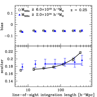
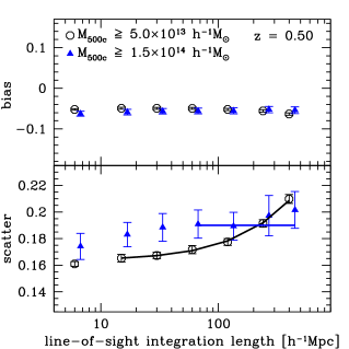
Figure 1.— The bias and scatter in WL mass measurements of $M_{500c}$ at $z=0.25$ (left) and $z=0.50$ (right). The open circles (black) and filled triangles (blue) show the results for halos satisfying the mass cuts given in the top panels for each redshift. The filled triangles are shifted by $+0.05$ dex in the horizontal direction for clarity. The lines show the predictions from Equation 12 in the regime where uncorrelated LSS along the LOS begins to have an effect on the scatter in the WL masses for each mass cut and redshift. See §4.1 for details concerning the fit of Equation 12 to the simulation data. The WL masses are clearly biased using for the NFW fitting and the behavior of the scatter as a function of LOS integration length is different for low- and high-mass halos. Note that a non-negligible fraction of the scatter and bias is due to correlated structures in matter distribution at distances between $\approx 6$ and $10$$h^{-1}\mathrm{Mpc}$ from the cluster.

We compute the errors and correlations of various quantities derived from the simulation and reduced tangential shear profile fits (e.g., the parameters of and scatter in the $M_{\mathrm{WL}}$-$M_{500c}$ relation) using a jackknife method. Namely, for the entire 1000 $h^{-1}\mathrm{Mpc}$ simulation box we split the two dimensions perpendicular to the LOS direction (i.e. the x-y plane perpendicular to the $z$-axis direction in our case) into a $10\times 10$ grid of one hundred $100\times 100$ $h^{-1}\mathrm{Mpc}$ cells. We can then use these cells to compute jackknife estimates of the covariance matrix of our desired quantities by not considering the halos in each cell in turn (see Scranton et al. 2002 for a similar technique).

4. Results

Our aim in this section is to illustrate the effect of the uncorrelated and correlated LSS on WL mass estimates and to give estimates for the scatter in WL-measured masses at fixed 3D mass under a variety of observational conditions. Our primary results in Figures 1–3 are discussed in detail in §4.1 and concern the intrinsic scatter and bias in WL mass estimates in the absence of galaxy shape noise. For these results we have chosen halos from the $z=0.25$ and $z=0.50$ snapshots and have used $\sigma_{\rm e}=0.3$ and $n_{\rm gal}=20$ galaxies/arcmin² to fix the error for each bin in the $\chi^{2}$-fitting metric. However we have not added shape noise (through Equation 9) to the reduced tangential shear profile in order to illustrate the intrinsic scatter and bias in the WL masses, as discussed in §3.2. Also, for these fiducial results we use 15 logarithmic bins in radius from the inner radial limit of 1 arcminute to an outer radial limit of $20$ arcminutes at $z=0.25$ and 10 logarithmic bins from 1 to 10 arcminutes at $z=0.50$. At $z=0.25$ our choice of outer radial fit limit matches approximately that used by Okabe et al. (2010a) for 30 low-redshift clusters. At $z=0.50$, we chose the outer radial fit limit of 10 arcminutes to match approximately that of the low-redshift halos relative to $r_{500c}$.

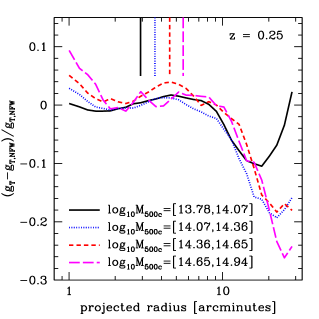
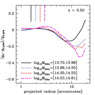
Figure 2.— Mean fractional difference between the reduced tangential shear profile predicted from an NFW fit to the three-dimensional mass profile of each halo, $g_{\rm T,NFW}$, and the halo’s true reduced tangential shear profile, $g_{\rm T}$. The average is taken in four bins of $\log M_{500c}$ for the $z=0.25$ (left) and $z=0.50$ (right) snapshots. The vertical lines extending from the top of each panel mark $r_{500c}$ for each halo mass bin. The range in $\log M_{500c}$ for each halo mass bin and the associated line style (and color) are given in the lower left corner of each panel. The virial radius of the halos in each mass bin is at $\approx 2r_{500c}$. The up turn at large radii is due to 2-halo contributions to the stacked shear signal. In the region between the 1- and 2-halo contributions beyond the halo virial radius, the NFW model is clearly wrong (see e.g., Tavio et al. 2008). Note that 1 arcminute corresponds to comoving distances of 206 $h^{-1}\mathrm{kpc}$ and 389 $h^{-1}\mathrm{kpc}$ at $z=0.25$ and $z=0.50$ respectively.

For our primary results, we fit for masses at an overdensity of 500 with respect to the critical density at the redshift of our halos. Qualitatively, the intrinsic scatter and bias in the WL masses for other overdensity mass definitions are similar. The effects of halo shape and orientation with respect to the LOS are discussed in §4.2. In §4.3, we give estimates for the scatter and bias in WL mass estimates under changing observational conditions, including varying overdensity fits, number of bins, maximum fit radius, source galaxy densities, and source galaxy shape noise. We emphasize again that the results of this section are specific to the method we have chosen for measuring the WL masses, even when we do not refer explicitly to our method itself. In §5 we will present a full discussion of our results in comparison to previous work.

4.1. Intrinsic Bias and Scatter in WL Mass Estimates

We will consider the distribution of WL masses at fixed 3D mass for a series of line-of-sight integration lengths in order to study the sources of bias and scatter. We will use integration lengths of 6, 15, 30, 60, 120, 240, and 400 $h^{-1}\mathrm{Mpc}$. An integration length of 400 $h^{-1}\mathrm{Mpc}$, for example, indicates that all the matter in the simulation from $-200$ $h^{-1}\mathrm{Mpc}$ to $+200$ $h^{-1}\mathrm{Mpc}$ along the LOS (with the cluster at zero) was included in constructing the reduced tangential shear profile. For each simulation snapshot and integration length we obtain a WL mass estimate of $M_{500c}$ for the cluster under consideration and can compare this WL mass estimate to the $M_{500c}$ mass measured in three dimensions.

Figure 1 shows the intrinsic scatter and bias in the WL masses as a function of LOS integration length for the population of halos at $z=0.25$ and $z=0.50$ snapshots. We have made two different mass cuts at each redshift to illustrate the difference between high- and low-mass halos. For the $z=0.25$ snapshot, we have kept the halos with $M_{500c}$ above $6.0\times 10^{13}h^{-1}\,{\it M}_{\odot}$ and $2.0\times 10^{14}h^{-1}\,{\it M}_{\odot}$ for the low and high mass halo samples respectively. For the $z=0.50$ snapshot the cuts were placed at $5.0\times 10^{13}h^{-1}\,{\it M}_{\odot}$ and $1.5\times 10^{14}h^{-1}\,{\it M}_{\odot}$. These mass thresholds are set so that the halo sample is complete above the low-mass threshold, so that there is approximately the same number of halos in the high-mass sample at both redshifts, and so that the qualitative differences in the shape of the scatter in the WL masses as a function of LOS integration length between the low- and high-mass halo samples are maximized.

The scatter, denoted as $\sigma_{\ln M_{\mathrm{WL}}}$, is the width of the best fit Gaussian to the residuals from a fit of the $\ln M_{\mathrm{WL}}$–$\ln M_{500c}$ relation of the form

$$\ln\left(\frac{M_{\mathrm{WL}}}{M_{p}}\right)=\beta+\alpha\ln\left(\frac{M_{500c}}{M_{p}}\right)\ .$$ (11)

The bias is defined as $\beta$ from the equation above and is the bias in $\langle\ln M_{\mathrm{WL}}|M_{500c}\rangle$. $M_{p}$ is a pivot mass chosen so that the errors on $\beta$ and $\alpha$ are uncorrelated. $\alpha$ is the slope of the relation. The covariance matrix of the quantities $\left\{\beta,\alpha,\sigma_{\ln M_{\mathrm{WL}}}\right\}$ is computed using the jackknife method described in §3.2. We have computed all of the correlations of the quantities $\left\{\beta,\alpha,\sigma_{\ln M_{\mathrm{WL}}}\right\}$ between the various LOS integration lengths and mass ranges using the jackknife method as well. The error bars shown in Figure 1 are the square-root of the diagonal elements of the jackknife covariance matrix. The best-fit parameters of Equation 11 for each mass threshold and snapshot using the 400 $h^{-1}\mathrm{Mpc}$ integration length for $M_{500c}$ are given in Table 1. The scatter in the WL masses listed in this table is extrapolated to the full LOS as described below.

In the method we adopt (i.e., the NFW profile fitting of the reduced tangential shear profile), the WL masses are on average biased low by $\approx 6\%$ in the $z=0.25$ and $z=0.50$ snapshots. A large portion, but not all, of the bias in the WL masses occurs because the NFW profile is a poor description of the actual shear profiles of clusters at the radii used in the fitting. We illustrate this issue as follows. For each halo we fit an NFW profile to the halo’s three-dimensional mass profile within $r_{500c}$. Then using the parameters from this fit, we predict the reduced shear profile, $g_{\mathrm{T,NFW}}$. In Figure 2 we have plotted the fractional difference between the true reduced shear profile, $g_{\mathrm{T}}$, and the prediction from the NFW fit of the three-dimensional halo mass profile, $(g_{\mathrm{T}}-g_{\mathrm{T,NFW}})/g_{\mathrm{T,NFW}}$ for cluster halos in different ranges of mass $M_{500c}$. Note that we compute the factional differences for each halo individually and then average over the mass bin. The lines at the top of the figure indicate the value of $r_{500c}$. The virial radius of each halo is $\approx 2r_{500c}$, which is well within 10 arcminutes for both analyzed redshifts for most clusters in the sample. Typical fits of the reduced tangential shear profile extend out to 10′-20′, where the actual reduced shear $g_{\mathrm{T}}$ deviates significantly from the predictions of the three-dimensional model. These deviations first become more negative as the density profile becomes steeper than the NFW profile in the cluster infall region. At larger radii the NFW model asymptotes to zero and the fractional deviations then become more positive due to 2-halo contributions of matter around the cluster.

A simple Monte Carlo estimate of the bias in the WL masses from the results of Figure 2 shows that fitting an incorrect model can account for $\approx 2-4\%$ of the bias in the WL masses at any overdensity and redshift. We make this estimate as follows. We generate reduced tangential shear profiles using a given mass and concentration of the cluster. We then introduce a bias in these profiles using the results of Figure 2. Then we fit the reduced tangential shear profile to determine a WL mass and compute the fractional bias in the WL mass. Our results indicate that using an improved fitting function, or limiting the radial range of the fits to the virial region, will decrease, but may not fully eliminate, the bias in our WL mass estimates.

There are other physical sources of bias in the WL masses, only some of which are included in Figure 2. Substructure in the outskirts of halos will cause the shear profile to deviate low at radii less than the radius of the substructure and will cause the shear profile to deviate high at radii greater than the substructure. This source of bias is already included in the estimates in Figure 2 since we are comparing the shear with all substructures in the simulation included to the expected shear from the three-dimensional halo profile. Additionally, averaging the WL masses estimated from spherically-symmetric NFW model fits to individual triaxial halos with different orientations along the LOS can produce a biased average WL mass at the level of a few percent for a single set of axis ratios (Corless & King 2007). However when the WL masses from fits to individual clusters are averaged over the entire population of halos with a range of axis ratios the net bias is small, $\approx 1\%$ high (Corless & King 2007). In addition to the effects of halo shape, the correlation between the halo major axis and the direction to nearby halos and filaments can potentially change the expected bias in the WL masses from this orientation averaging effect as well. Our simulations include all of these correlations automatically and so are a useful tool for studying these effects in aggregate.

Note also that the bias in the WL masses depends sensitively on the fitting method. If we use the $\chi^{2}_{\rm uw}$ or $\chi^{2}_{\rm abs}$ fitting metrics, the WL masses are only biased low by $\approx 3-4\%$. These metrics tend to weigh the inner bins of the reduced tangential shear profile in the fit more than a pure $\chi^{2}$ fitting metric. The reduced tangential shear profile is biased less in the inner regions in Figure  2, so that the WL masses tend to be less biased using these alternative fitting metrics.

We additionally find that the exact choice of halo center can have a strong effect on the bias in the WL masses. For example, if we allow the halo centers to move randomly $\pm 100$ $h^{-1}\mathrm{kpc}$ comoving in the two orthogonal directions in the projected halo field about the fiducial center defined by the halo finder, the bias increases to $\approx 7-10\%$ low for the 400 $h^{-1}\mathrm{Mpc}$ integration length at $z=0.25$. We can also search for the peak of the convergence field for each halo. We search the region defined by $\pm 12$ grid cells about the grid center ($\pm 469$ $h^{-1}\mathrm{kpc}$ in comoving distance) for the peak of the convergence field for the 400 $h^{-1}\mathrm{Mpc}$ integration length at $z=0.25$. In this case, the peak tends to be approximately two grid cells (78 $h^{-1}\mathrm{kpc}$ comoving) or less away from the fiducial halo center defined by the halo finder. The bias in the WL masses increases by $\lesssim 1\%$ using these new halo centers. Thus we can conclude that the halo centers defined by our halo finder are robust in this regard. The effect of halo centering on the bias in the WL masses is quite sensitive to the exact choice of inner fitting radius as shown by Hoekstra et al. (2011a). We do not explore this dependence in this work.

Table 1Intrinsic Relation Between Weak Lensing Mass Estimates of $M_{500c}$and 3D Mass.

$M_{p}$	$\beta$	$\alpha$	$\sigma_{\ln M_{\mathrm{WL}}}$
$z=0.25$, $M_{500c}\geq 6.0\times 10^{13}h^{-1}\,{\it M}_{\odot}$
$9.74\times 10^{13}h^{-1}\,{\it M}_{\odot}$	$-0.059\pm 0.003$	$0.997\pm 0.006$	$0.297\pm 0.008$
$z=0.25$, $M_{500c}\geq 2.0\times 10^{14}h^{-1}\,{\it M}_{\odot}$
$2.80\times 10^{14}h^{-1}\,{\it M}_{\odot}$	$-0.052\pm 0.007$	$0.99\pm 0.03$	$0.207\pm 0.005$
$z=0.50$, $M_{500c}\geq 5.0\times 10^{13}h^{-1}\,{\it M}_{\odot}$
$7.89\times 10^{13}h^{-1}\,{\it M}_{\odot}$	$-0.063\pm 0.003$	$1.001\pm 0.007$	$0.311\pm 0.009$
$z=0.50$, $M_{500c}\geq 1.5\times 10^{14}h^{-1}\,{\it M}_{\odot}$
$2.07\times 10^{14}h^{-1}\,{\it M}_{\odot}$	$-0.054\pm 0.008$	$0.96\pm 0.03$	$0.22\pm 0.01$

The slope $\alpha$ of the relation in Equation 11 is generally consistent with unity at large LOS integration lengths. However there are $\gtrsim 3\sigma$ deviations of the slope below or above unity in some mass ranges, especially at the smallest LOS integration length in each snapshot for both mass bins. A relation with a slope significantly different than unity would indicate that the bias in the WL masses depends on the halo mass. However, as shown in Figure 2, the deviation of the reduced tangential shear profiles from the NFW model are nearly the same over all of the mass bins, consistent with the slope of the $M_{\mathrm{WL}}$-$M_{500c}$ being close to unity.

As the LOS integration length is increased, so does the scatter in the WL masses. The scatter for the low-mass halo sample increases more strongly than that for the high-mass halo sample in both snapshots. Note that correlated structures at distances $\approx 3-10$ $h^{-1}\mathrm{Mpc}$ contribute to the scatter. This correlated structure is not due to the triaxiality of the cluster itself, but is due to neighboring groups, clusters, and filaments. At distances $\gtrsim 10$ $h^{-1}\mathrm{Mpc}$, the scatter is generated from a superposition of many largely uncorrelated structures.

We propose a simple toy model of the scatter as a function of mass and LOS integration length which can explain the trends in Figure 1. We assume that the scatter in the WL masses due to uncorrelated LSS is proportional to the scatter in the shear. We compute the fractional scatter in the WL masses as

$$\frac{\Delta M_{\mathrm{WL}}}{M_{\mathrm{WL}}}=\frac{\sqrt{\left[fM_{\rm med}\right]^{2}+\left[A\sigma_{\rm LSS}(d)\right]^{2}}}{M_{\rm med}}$$ (12)

where $f$ is the fractional intrinsic scatter in the WL masses due to halo triaxiality and correlated LSS, $\sigma_{\rm LSS}(d)$ is the scatter in the shear due to uncorrelated LSS as a function of the LOS integration length $d$, and $A$ is a proportionality constant with units of $h^{-1}\,{\it M}_{\odot}$ that is independent of the LOS integration length $d$ and halo mass. $M_{med}$ is the median halo mass of the sample under consideration. The form of this model is motivated by the fact that scatter from uncorrelated LSS should simply add in quadrature to the scatter from triaxial halo shapes and correlated LSS. We compute $\sigma_{\rm LSS}(d)$ as a function of integration length using the results of Hoekstra (2003) with the transfer function from Eisenstein & Hu (1998) and the non-linear matter power spectrum from Smith et al. (2003). In general, $\sigma_{\rm LSS}(d)$ depends on the radius and width of the annulus used to average the tangential shear. However, as shown in Hoekstra (2003), this dependence is not strong. We use a bin of radius 10 arcminutes with a width much less than the radius to get a representative value. For each snapshot this model is fit the to the last four LOS integration length points (i.e. 60, 120, 240 and 400 $h^{-1}\mathrm{Mpc}$) for both mass bins simultaneously using the jackknife covariance matrix computed above. We assume that both mass bins have the same value of $A$, but different values of $f$, $f_{\rm low}$ and $f_{\rm high}$, for a total of three free parameters per snapshot and five degrees of freedom in the fit.

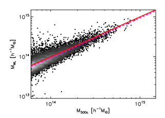
Figure 3.— Left: Scatter-contour plot of $M_{500c}$obtained from fitting the reduced tangential shear profile, $M_{\mathrm{WL}}$, against the 3D $M_{500c}$ mass measured in the simulation. The “high-density” regions of the plot are shown with grey shaded contours (light to dark indicates high- to low-density) and the rest of the data is shown as points. The solid (red) line marks a one-to-one ratio and the dashed (magenta) line is the best-fitting power-law given in Equation 11. The best-fit power law is biased low by $\approx 6\%$ but the slope is consistent with unity. Right: Residuals from the best-fitting power law on the left. The solid line is the best-fitting Gaussian model to the residuals in $\ln M_{500c}$. The skewness of the residuals, $0.70\pm 0.14$, is clearly non-zero indicating that the conditional distribution of $M_{\mathrm{WL}}$ at fixed $M_{500c}$ is close to, but not quite log-normal. See §4.1 for details.

The fractional scatter predicted by Equation 12 for the low- and high-mass sample of halos is shown as the solid lines in Figure 1. We have plotted model predictions for points not used to fix the value of $A$, $f_{\rm low}$, and $f_{\rm high}$ for the low mass bins in each snapshot as well. While the specific value of $A$ is somewhat arbitrary, the values of $f_{\rm low}$ and $f_{\rm high}$ for each snapshot indicate the total amount of scatter due to halo triaxiality and correlated LSS. The three parameters for the $z=0.25$ snapshot are $A=(7.5\pm 0.3)\times 10^{15}h^{-1}\,{\it M}_{\odot}$, $f_{\rm low}=0.170\pm 0.002$, and $f_{\rm high}=0.189\pm 0.006$. For the $z=0.50$ snapshot the parameters are $A=(6.6\pm 0.3)\times 10^{15}h^{-1}\,{\it M}_{\odot}$, $f_{\rm low}=0.163\pm 0.003$, and $f_{\rm high}=0.19\pm 0.01$. Figure 1 shows that about $80\%$ of the scatter $f$ is due to matter within $\approx 3$ $h^{-1}\mathrm{Mpc}$ of clusters (i.e., within $2-3$ virial radii) and $\approx 20\%$ is due to the matter in correlated structures between 3 and 10 $h^{-1}\mathrm{Mpc}$.

This model summarizes nicely the way in which uncorrelated LSS along the LOS effects WL masses. Uncorrelated LSS along the LOS adds approximately the same amount of scatter to mass estimates independent of halo mass. Thus, in terms of fractional scatter, low-mass halos are more strongly affected by uncorrelated LSS along the LOS because they produce less shear as compared to high-mass halos. This fact motivates the assumption that parameter $A$ is the same for low- and high-mass halos.

The differences between $f_{\rm low}$ and $f_{\rm high}$ for the different cluster mass thresholds and snapshots are harder to explain with a simple model. They are essentially due to changes in halo bias and shape as a function of mass. Less massive halos tend to be more spherical (see e.g., Allgood et al. 2006) than more massive halos. Thus the fractional scatter generated by averaging over many orientations is smaller for lower mass halos. Additionally, higher mass halos are more biased with respect to the dark matter than lower mass halos (see Tinker et al. 2010 for a recent study of halo bias). Therefore, contributions to the scatter in the WL masses from correlated structure outside the virial radius (i.e. any slight increase in the scatter from an LOS integration length of 6 to $\approx 120$ $h^{-1}\mathrm{Mpc}$) along the LOS generally are stronger for more massive halos. Based on the changes in the scatter as function of LOS distance in Figure 1, the effects of halo shape seem to be dominant in determining $f_{\rm low}$ and $f_{\rm high}$. However, as we noted above, the effects of correlated LSS outside the virial radius are not negligible.

Additionally, the model in Equation 12 can be used to extrapolate the scatter measured in the simulations over a restricted LOS to the full LOS. We simply evaluate the model using the value of $\sigma_{\rm LSS}(d)$ from integrating over the entire LOS from the observer to the sources at redshift one. The results are given in Table 1 for both snapshots and mass bins. The extrapolated scatter values represent the total amount of intrinsic scatter in WL mass estimates of $M_{500c}$ for our fitting method from all sources along the LOS to redshift $z=1$. Note that this extrapolation and the resulting effects of uncorrelated LSS on the scatter in the WL masses will change if the source galaxies extend to higher redshifts.

Finally, in Figure 3 we show a contour-scatter plot of the $\ln M_{\mathrm{WL}}$-$\ln M_{500c}$ relation and a histogram of the residuals about the best-fit power law for the $z=0.25$ snapshot at the 400 $h^{-1}\mathrm{Mpc}$ integration length. We have used all halos with $M_{500c}\geq 6.0\times 10^{13}h^{-1}\,{\it M}_{\odot}$ for this plot. There is a small number of halos in the simulation where the WL mass differs from the 3D mass by a factor of five or more (the outliers in the left panel of Figure 3). We have visually checked the reduced shear profiles of these halos and found that they are negative in one or more bins and/or are strongly non-monotonic. These pathological cases are due to the presence of a second mass peak in the shear field which cancels shear from the main peak associated with the halo.

The conditional distribution of the WL masses from the best-fit mean relation shown in the right panel of Figure 3 is close to log-normal. However there is a statistically significant tail at high WL masses. The skewness of the distribution in the right panel of Figure 3 is $0.70\pm 0.14$ for halos with $M_{500c}\geq 6.0\times 10^{13}h^{-1}\,{\it M}_{\odot}$. For the higher mass sample with $M_{500c}\geq 2.0\times 10^{14}h^{-1}\,{\it M}_{\odot}$, the conditional distribution is somewhat closer to log-normal with skewness $0.38\pm 0.11$. The conditional distribution at $z=0.50$ is quite similar with skewness $0.43\pm 0.18$ for the low mass sample with $M_{500c}\geq 5.0\times 10^{13}h^{-1}\,{\it M}_{\odot}$ and $0.49\pm 0.12$ for the high mass sample with $M_{500c}\geq 1.5\times 10^{14}h^{-1}\,{\it M}_{\odot}$.

4.2. The Effects of Halo Shape and Orientation

We have also investigated the correlation between the orientation of the halo with respect to the LOS and the deviation of its WL mass from the mean relation as a function of LOS integration length. Specifically, we compute the correlation coefficient between $\cos\theta$ and $\Delta\ln M_{\mathrm{WL}}=\ln M_{\mathrm{WL}}-\left\langle\ln M_{\mathrm{WL}}|M_{500c}\right\rangle$. Here $\theta$ is the angle of the halo’s major axis with respect to the LOS (see §2 for details) and $\left\langle\ln M_{\mathrm{WL}}|M_{500c}\right\rangle$ is the best-fit mean relation defined in Equation 11. This correlation coefficient is $\approx 0.68$ at the LOS integration length 6 $h^{-1}\mathrm{Mpc}$ and declines to $\approx 0.51$ at 400 $h^{-1}\mathrm{Mpc}$ for the low mass halo sample defined above from the $z=0.25$ snapshot. For the high mass halo sample from the same snapshot, the correlation coefficients at 6 and 400 $h^{-1}\mathrm{Mpc}$ are $\approx 0.72$ and $\approx 0.61$ respectively. The correlation coefficient between $\cos\theta$ and $\Delta\ln M_{\mathrm{WL}}$ is smooth and monotonic from 6 to 400 $h^{-1}\mathrm{Mpc}$. For the high mass halos, the correlation coefficient shows a slight increase from 3 to 6 $h^{-1}\mathrm{Mpc}$ as the LOS integration length increases to include all of the halo’s mass. Similar trends are seen in the $z=0.50$ snapshot.

The correlation coefficients decrease as the LOS integration length is increased because of random perturbations to the shear profiles due to uncorrelated LSS or due to imperfect alignment of correlated structures. The decline is stronger for lower mass halos because they produce less shear, so that random perturbations have a larger effect. In addition to the fact that smaller halos produce less shear, it is known that the orientation of halos is correlated with the orientation of the filamentary structure around them (see §1 for references). Thus the filamentary, correlated LSS around larger halos, which are more highly biased, will work to maintain the correlation coefficient as the LOS integration length is increased.

Table 2Bias and Scatter in Weak Lensing Masses Estimates of $M_{500c}$ at $z=0.25$.

maximum fit radius	12 bins		15 bins		17 bins		20 bins
	$\{\sigma_{\rm e},n_{\rm gal}\}=\{0.3,10\}$
	Bias	Scatter	Bias	Scatter	Bias	Scatter	Bias	Scatter
15$\arcmin$	-0.06$\pm$0.01	0.38$\pm$0.02	-0.06$\pm$0.01	0.39$\pm$0.02	-0.08$\pm$0.01	0.34$\pm$0.02	-0.08$\pm$0.01	0.35$\pm$0.02
20$\arcmin$	-0.09$\pm$0.01	0.34$\pm$0.02	-0.10$\pm$0.02	0.37$\pm$0.04	-0.09$\pm$0.01	0.33$\pm$0.03	-0.10$\pm$0.01	0.36$\pm$0.03
25$\arcmin$	-0.11$\pm$0.01	0.34$\pm$0.03	-0.10$\pm$0.01	0.37$\pm$0.02	-0.12$\pm$0.01	0.33$\pm$0.02	-0.10$\pm$0.01	0.35$\pm$0.03
	$\{\sigma_{\rm e},n_{\rm gal}\}=\{0.3,20\}$
	Bias	Scatter	Bias	Scatter	Bias	Scatter	Bias	Scatter
15$\arcmin$	-0.06$\pm$0.01	0.29$\pm$0.01	-0.05$\pm$0.01	0.29$\pm$0.02	-0.06$\pm$0.01	0.28$\pm$0.02	-0.07$\pm$0.01	0.27$\pm$0.02
20$\arcmin$	-0.07$\pm$0.01	0.27$\pm$0.02	-0.07$\pm$0.01	0.29$\pm$0.02	-0.08$\pm$0.01	0.29$\pm$0.02	-0.08$\pm$0.01	0.29$\pm$0.02
25$\arcmin$	-0.09$\pm$0.01	0.29$\pm$0.02	-0.10$\pm$0.01	0.29$\pm$0.02	-0.09$\pm$0.01	0.27$\pm$0.02	-0.10$\pm$0.01	0.28$\pm$0.02
	$\{\sigma_{\rm e},n_{\rm gal}\}=\{0.3,40\}$
	Bias	Scatter	Bias	Scatter	Bias	Scatter	Bias	Scatter
15$\arcmin$	-0.05$\pm$0.01	0.26$\pm$0.02	-0.05$\pm$0.01	0.26$\pm$0.02	-0.05$\pm$0.01	0.25$\pm$0.02	-0.05$\pm$0.01	0.27$\pm$0.01
20$\arcmin$	-0.06$\pm$0.01	0.24$\pm$0.02	-0.07$\pm$0.01	0.25$\pm$0.02	-0.06$\pm$0.01	0.24$\pm$0.01	-0.07$\pm$0.01	0.23$\pm$0.02
25$\arcmin$	-0.07$\pm$0.01	0.26$\pm$0.01	-0.07$\pm$0.01	0.22$\pm$0.02	-0.08$\pm$0.01	0.24$\pm$0.01	-0.08$\pm$0.01	0.25$\pm$0.01

It is interesting that even considering all matter between $-200$ and $+200$ $h^{-1}\mathrm{Mpc}$, the correlation coefficients are still substantial, $\approx 0.50-0.60$. We expect the correlation coefficients to decrease more as the LOS integration length is increased, but extrapolating accurately to the final values for a full LOS from the simulation data we have presented here is difficult. However, we can do this extrapolation approximately as follows. We use the toy model proposed in Equation 12 above to include the effects of uncorrelated LSS along the LOS on the WL masses. The term proportional to $(A\sigma_{\rm LSS}(d)/M_{\rm med})^{2}$ in Equation 12 is the extra variance introduced into the WL masses due to the effects of uncorrelated LSS projections along the LOS. We thus use log-normal random deviates with variance equal to $(A\sigma_{\rm LSS}(d)/M_{500c})^{2}$ and zero mean to add scatter to the WL masses in order to simulate the effects of LSS projections along the LOS not included in our simulation box. Here we use the value of $\sigma_{\rm LSS}(d)$ which corresponds to the extra scatter due to a full LOS from lensing sources to the observer and $M_{500c}$ is set to the 3D mass of each cluster individually when adding the random scatter. We start with the WL masses at an integration length of 120 $h^{-1}\mathrm{Mpc}$. The choice of starting integration length is motivated by the fact that most of the correlated structure along the LOS due to filamentary LSS is within 60-100 $h^{-1}\mathrm{Mpc}$ of the halo center. We then recompute the correlation coefficients. We find a correlation coefficient of $\approx 0.37$ for the low-mass bins in both the $z=0.25$ and $z=0.50$ snapshots. For the high-mass bins in both snapshots, the correlation coefficients are $\approx 0.58$. If we use the WL masses at an integration length of 240 $h^{-1}\mathrm{Mpc}$, these numbers change by $\lesssim 0.01$, indicating that our extrapolation is robust to this choice.

While there is certainly some uncertainty in this extrapolation, it is clear that the correlation still remains positive even integrating over a full LOS. Stated differently, the key point is that the sign (i.e. positive or negative) of the deviation of the WL mass from the 3D mass is on average set by the orientation of the matter within and near the virial radius of the halo. Matter outside the virial radius of the halo along the LOS changes the strength of the correlation between the orientation of the halo and the deviations of the WL masses from the 3D masses, but the correlation is always positive at high significance on the scales probed by our simulation and remains positive even after extrapolating to a full LOS.

In addition to halo orientation with respect to the LOS, halo shapes also influence the WL masses. To investigate this effect, we build subsamples of halos which are more spherical or more triaxial based on the minor to major axis ratio, denoted here as $S$ (see §2 for details concerning its computation). We fit a power-law to the mean value of $S$ as a function of $M_{500c}$ (a similar relation was used in Allgood et al. 2006). Using the mean power-law relation between $S$ and $M_{500c}$, we compare all halos with $S$ in the upper quartile of the distribution of $S$ at fixed mass (i.e. the more spherical halos) to the entire halo population and all halos with $S$ in the lower quartile of the distribution of $S$ at fixed mass (i.e. the more triaxial halos) to the entire halo population using the same mass bins as before. These cuts generate four halo samples per snapshot.

We find that while the bias in normalization and slope of the $M_{\mathrm{WL}}$-$M_{500c}$ relations are unaffected in a statistically significant way by cuts on halo shape, the scatter in the WL masses does depend on halo shape. Not unexpectedly, the WL masses of more spherical halos have less scatter than those of more triaxial halos. In both snapshots for the low-mass cuts, the more triaxial halos have $\approx 3-5\%$ more scatter than the entire halo population while the more spherical halos have $\approx 3-5\%$ less scatter than the entire halo population. For the high-mass cuts the mean shifts in the scatter between the different samples are the same, but the trend is not statistically significant given the jackknife errors. We find additionally that the difference in the scatter in the WL masses between the more spherical halos and the entire population increases marginally with integration length from 60 $h^{-1}\mathrm{Mpc}$ to 400 $h^{-1}\mathrm{Mpc}$ in the $z=0.50$ snapshot. Given that correlations between halo orientation and LSS persist out to $\sim 100$ $h^{-1}\mathrm{Mpc}$ and that spherical halos tend to be more highly biased (i.e. more clustered) than triaxial halos at fixed mass (Faltenbacher & White 2010) and thus tend to dominate their local environment more strongly, this trend is physically plausible.

4.3. Scatter and Bias Under Varying Observational Conditions

In this section we present the bias and scatter in the WL masses at fixed 3D mass including the effects of galaxy shape noise. For each halo in the simulation, we vary the source density, amount of shape noise, maximum radius of the fit, and the number of bins used in the fit. We consider WL mass estimates of $M_{200m}$, $M_{200c}$, and $M_{500c}$. For each set of observational parameters and mass overdensity definition, we measure the bias and scatter in the WL masses. Since we are now including observational errors in the reduced tangential shear profiles, the shear of some of the lower mass halos will be undetectable. We thus focus only on the highest mass halos in the simulation which have the highest signal-to-noise.

Additionally, we find that in the presence of observational errors, even while focusing on the high-mass halos only, there are still outliers in the WL masses, especially for the poorest observations with $\{\sigma_{\rm e},n_{\rm gal}\}=\{0.3,10\}$. These outliers generally occur when the signal-to-noise is low so that the WL mass differs from the 3D mass by a factor of five or more and is biased low. We thus cut all halos where the WL mass differs from the 3D mass by a factor of five or more before computing the bias and scatter in the WL masses. These cuts reject low signal-to-noise observations while still retaining a sample with a sharp mass threshold above which the sample is nearly $100\%$ complete. We do not use direct cuts on signal-to-noise since these cuts result in a sample with varying completeness as a function of mass. This extra cut has a negligible effect on the results at $z=0.25$, but does reduce the measured bias in the WL masses at $z=0.50$.

The bias and scatter in the WL mass measurements of $M_{500c}$ averaged over all halos with $M_{500c}\geq 2.0\times 10^{14}h^{-1}\,{\it M}_{\odot}$ at $z=0.25$ are given in Table 2. We show results for different outer radial limits of the fit and the number of bins for the errors typical for a wide-area DES-like, deep ground-based, and space-based observational surveys. The scatter in the WL mass varies as a function of the quality of the observations, but varies very little with the exact choice of outer radial fit limit or number of bins. The expected scatter in WL mass estimates of $M_{500c}$ at fixed 3D mass for very common ground-based or DES-like observations is $\approx 33-39\%$. For current common ground-based or DES-like observations, the dominant source of scatter is shape noise from background galaxies. For deeper ground-based observations, the scatter drops slightly to $\approx 27-29\%$. For high-quality observations like those expected from LSST or space-based instruments, the scatter drops to $\approx 22-27\%$. As the number density of sources approaches that expected from space-based observations or LSST, the contribution to the scatter in the WL masses from galaxy shape noise becomes comparable or even sub-dominant to the intrinsic scatter in the WL masses at $z=0.25$ for the radial fitting ranges we have considered here. If the radial fitting range is decreased significantly (e.g. to 10 arcminutes), the scatter in the WL masses will increase even for the highest quality observations simply because many fewer galaxies are used in the measurement and thus the signal-to-noise is lower.

Table 3Bias and Scatter in Weak Lensing Masses Estimates of $M_{200m}$, $M_{200c}$, and $M_{500c}$at $z=0.25$.

mass definition $\Delta\rho(z)$	Bias	Scatter
	$\{\sigma_{\rm e},n_{\rm gal}\}=\{0.3,10\}$
$200\rho_{m}(z)$	+0.00$\pm$0.02	0.40$\pm$0.02
$200\rho_{c}(z)$	-0.06$\pm$0.01	0.35$\pm$0.01
$500\rho_{c}(z)$	-0.10$\pm$0.02	0.37$\pm$0.04
	$\{\sigma_{\rm e},n_{\rm gal}\}=\{0.3,20\}$
$200\rho_{m}(z)$	+0.02$\pm$0.01	0.32$\pm$0.02
$200\rho_{c}(z)$	-0.06$\pm$0.01	0.27$\pm$0.02
$500\rho_{c}(z)$	-0.07$\pm$0.01	0.29$\pm$0.02
	$\{\sigma_{\rm e},n_{\rm gal}\}=\{0.3,40\}$
$200\rho_{m}(z)$	+0.02$\pm$0.01	0.27$\pm$0.02
$200\rho_{c}(z)$	-0.04$\pm$0.01	0.25$\pm$0.01
$500\rho_{c}(z)$	-0.07$\pm$0.01	0.25$\pm$0.02

Table 4Bias and Scatter in Weak Lensing Masses Estimates of $M_{200m}$, $M_{200c}$, and $M_{500c}$at $z=0.50$.

mass definition $\Delta\rho(z)$	Bias	Scatter
	$\{\sigma_{\rm e},n_{\rm gal}\}=\{0.3,10\}$
$200\rho_{m}(z)$	+0.03$\pm$0.03	0.52$\pm$0.07
$200\rho_{c}(z)$	-0.04$\pm$0.02	0.57$\pm$0.03
$500\rho_{c}(z)$	-0.11$\pm$0.02	0.51$\pm$0.04
	$\{\sigma_{\rm e},n_{\rm gal}\}=\{0.3,20\}$
$200\rho_{m}(z)$	-0.04$\pm$0.03	0.44$\pm$0.06
$200\rho_{c}(z)$	-0.08$\pm$0.02	0.42$\pm$0.05
$500\rho_{c}(z)$	-0.10$\pm$0.01	0.40$\pm$0.03
	$\{\sigma_{\rm e},n_{\rm gal}\}=\{0.3,40\}$
$200\rho_{m}(z)$	+0.02$\pm$0.02	0.32$\pm$0.08
$200\rho_{c}(z)$	-0.06$\pm$0.01	0.36$\pm$0.03
$500\rho_{c}(z)$	-0.09$\pm$0.01	0.33$\pm$0.02

The bias in the WL masses at fixed 3D mass is in the range of $[-12\%,-5\%]$ in all cases at $z=0.25$. The errors in the bias from the jackknife samples are typically $\approx\pm 1\%$ for the high-mass halo sample we are considering. The bias generally increases with increasing outer radial fit limit. The main cause of this bias is apparent in Figure 2: the deviation of the halo’s true tangential shear profile from the NFW model we are using in our fitting method increases as the outer fit limit is increased, resulting in more bias in the WL masses. We have confirmed this trend using the Monte Carlo method described above.

For reference, the bias and scatter in WL mass measurements for various other mass definitions at $z=0.25$ are given in Table 3. For this table we have set the outer radial limit of the fit to 20 arcminutes and the number of bins to 15. The shape noise contribution to the scatter in the WL masses is dominant for all mass definitions. The scatter increases as the overdensity decreases because smaller overdensities pivot the fit of the tangential shear profile away from the median observed radius (Okabe et al. 2010a). The shift in the pivot point causes uncertainty in the measured concentration of the NFW profile to project into the WL mass, causing the scatter to increase.

The bias and scatter in the WL masses using an outer fit limit of 10 arcminutes and 10 bins for $z=0.50$ are given in Table 4. The biases in the WL masses in the presence of shape noise for common ground-based observations are marginally larger at $z=0.50$ than at $z=0.25$. Also there is significantly more scatter in the WL masses at $z=0.50$, due to the decreased radial range of the fits and the corresponding drop in signal-to-noise of the WL mass measurements.

Weak lensing masses measured at an overdensity of $\Delta\rho(z)=200\rho_{m}(z)$ seem to be unbiased at both $z=0.25$ and $z=0.50$. Additionally, if we use 10 bins and an outer fit limit of 10 arcminutes for the $z=0.25$ halos, then the WL masses measured at $\Delta\rho(z)=500\rho_{c}(z)$ are nearly unbiased, $-0.01\pm 0.01$ for $\{\sigma_{\rm e},n_{\rm gal}\}=\{0.3,40\}$, as one would expect from Figure 2. However, with the 10 arcminute outer fit limit for the $z=0.25$ halos, the WL masses measured at lower overdensities are then biased high, $0.06\pm 0.01$ for $M_{200c}$ and $0.10\pm 0.02$ for $M_{200m}$ with $\{\sigma_{\rm e},n_{\rm gal}\}=\{0.3,40\}$. The apparent discrepancies between these results and Figure 2 occur because the NFW fits of the three-dimensional mass profile were done within $r_{500c}$ only. Thus while Figure 2 reflects the differences between the observed shear profiles and the NFW prediction for $M_{500c}$, NFW fits of the three-dimensional mass profile within $r_{200c}$ or $r_{200m}$ would be different, and thus this figure for the lower over density mass definitions would change. Thus Figure 2 is only applicable to the biases in WL estimates of $M_{500c}$.

4.4. Tests of a Iterative Strategy for Mitigating Biases in WL Mass Estimates

As discussed in the previous section, the biases in the WL masses depend principally on how far in radius the fit to the reduced tangential shear profile is carried out. Given that the source of the bias are deviations of the actual mass distribution from the NFW form outside the virial radius of the halo, one may wonder then whether the bias can be removed by restricting the fits to radii within the virial radius only. We have tested a simple algorithm of iteratively determining the outer radial fit limit from the measured WL mass. Specifically, we first fit the reduced tangential shear profile within some fiducial outer fit radius, 20 arcminutes for halos at $z=0.25$ and 10 arcminutes for halos at $z=0.50$. We then use the WL mass estimate resulting from such fit to refit the reduced tangential shear profile within the virial radius from the previous fit (i.e., $r_{500c}$ for $M_{500c}$, $r_{200m}$ for $M_{200m}$, etc.). This process is repeated until the WL mass converges, usually after a few iterations.

For halos at $z=0.25$ above the mass limits listed in Table 3, the bias in the WL masses over all halo definitions and observational conditions using such an iterative fitting method is in the range of $[-10\%,+8\%]$ with a $1\sigma$ error in the range of $2-3\%$. The average absolute bias in units of the jackknife errors is $2.6\sigma$ for the iterative fitting method as compared to $4.2\sigma$ for the biases listed in Table 3 (a fixed outer radial fit limit of 20 arcminutes). Note that this improvement is driven mostly by the increase in the jackknife errors and corresponding increases in the scatter in the WL masses, since the average absolute biases for these two methods are nearly identical around $\sim 5\%$.

The iterative method does improve the estimate of masses defined within radii enclosing relatively high overdensity. Thus, for $M_{500c}$ at $z=0.25$ and $n_{\rm gal}\gtrsim 20$, the iterative fitting method results in average bias of only $-2.5\pm 2.0\%$, i.e. no significant bias. This is consistent with the results in the previous section for WL mass estimates of $M_{500c}$ with an outer radial fit limit of 10 arcminutes at $z=0.25$. The results for lower source densities with $M_{500c}$ at $z=0.25$ are somewhat inconclusive because error bars on the mean bias are considerably large in this case. Due to large errors, the bias in $M_{500c}$, $-10\pm 3\%$ is still consistent with zero for such source densities.

At $z=0.50$ for halos above the mass limits listed in Table 4, the iterative method shows only a small improvement over results for a fixed outer fit limit of 10 arcminutes, even for $M_{500c}$. We find that $M_{500c}$ is biased by the same amount on average over all source densities, $-10\pm 2\%$, for both the iterative method and for the fixed outer fit limit. Given that Figure 2 shows that model NFW tangential shear profiles should be unbiased at $r\lesssim r_{500c}$, the bias must be due to convergence of the method to incorrect $r_{500c}$ radius. Indeed, given that we start the method with profile fitted within 10 arcminutes, at which the model profiles are highly biased, convergence to the correct radius is not guaranteed. If a measurement of $M_{500c}$ is the goal, the WL mass measurements should therefore be restricted to even smaller radii to avoid biases, even though this will result in degradation of the signal-to-noise of the measurements. For $M_{500c}$, we find that by starting the iterative fitting method at 5 arcminutes, the biases drop to $-2\pm 2\%$ on average over all source densities. For masses defined within radii enclosing over densities lower than $500c$, the iterative fitting results in biased mass estimates with the bias in the range of $[-13\%,+7\%]$ with a $1\sigma$ error of $2-5\%$. While the bias is consistent with zero according to the error bars, the errors bars are large enough that we cannot distinguish changes in the biases at high precision. These results are thus inconclusive for over densities lower than $500c$.

Overall our results indicate that the bias in the WL masses can be alleviated for $M_{500c}$ measurements by restricting fits to smaller angular scales, and iteratively decreasing the outer fit radius to converge to $r_{500c}$, although care must be taken to perform fits only within radii where NFW model is expected to be an unbiased model for the shear ($\lesssim 10^{\prime}$ at $z=0.25$ and $\lesssim 5^{\prime}$ at $z=0.5$, see Fig. 2). However, this method does not eliminate biases for other mass definitions enclosing lower overdensities and other methods will need to be explored to eliminate bias in mass measurements within larger radii.

5. Discussion

Our results presented in the previous section show that contributions to the scatter and bias in WL masses estimated from an NFW fit comes from three physically distinct sources: matter within the halo virial radius, correlated LSS at distances 6-20 $h^{-1}\mathrm{Mpc}$ from clusters, and uncorrelated LSS at larger distances. Previous studies have used a combination of analytic models and simulations to study these different sources separately, while we have considered the effects of all three simultaneously. In the subsections below, we summarize the contributions of each of these sources and compare to various previous studies of this subject. We also discuss in detail some implications of our results for studies of cosmology with galaxy clusters.

5.1. Matter Within the Halo Virial Radius

The matter within the virial radius and immediately outside of it is a significant source of scatter and the main source of biases in the WL mass estimates using NFW fits. Specifically, the bias shown in Figure 1 changes negligibly once the LOS integration length is increased beyond 6 $h^{-1}\mathrm{Mpc}$. The main origin of the bias is shown in Figure 2, which shows that deviations of the mean reduced tangential shear profile from NFW profile are significant outside the virial radius. So when these radii are included in the NFW fit, the resulting mass is biased low. The deviations in Figure 2 are consistent with the results of Tavio et al. (2008), who have systematically studied density profiles of halos beyond the virial radius.

In addition to demonstrating that using an inaccurate density profile can bias WL mass estimates, we have demonstrated that even if the correct halo profile is known, there are still biases in the WL masses which depend on the specific details of the fitting method and need to be calibrated in simulations. Note that high-resolution simulations naturally include other sources of bias like substructure, halo triaxiality, and potential halo centering issues as well. Specifically, we have demonstrated in our simulations that halo centering errors can introduce $\approx 5\%$ negative biases in WL masses as has been seen before using analytic models (see e.g., Hoekstra et al. 2011a). The myriad of complications involved in WL mass estimation makes detailed studies of shear fitting using shear fields derived from cosmological simulations indispensable in estimating the bias and scatter of the weak lensing mass measurements.

The orientation of the major axis of halo mass distribution also affects the magnitude and sign of the bias in the WL mass estimates. This effect was discussed by Clowe et al. (2004) for a small sample of simulated clusters using all matter within 7.5 $h^{-1}\mathrm{Mpc}$ of the halo center. Meneghetti et al. (2010b) have detected this effect with a similarly small sample of halos using all matter within 10 $h^{-1}\mathrm{Mpc}$ of the halo center. Finally, Oguri et al. (2005) and Corless & King (2007) used analytic triaxial NFW models to arrive at a similar conclusion for matter within the halo virial radius. We have extended this type of analysis to the full LOS, showing that these correlations persist to large distances, and to a much larger sample of simulated halos.

Halos in the roundest quartile of the distribution of $S$ at fixed mass have less scatter in the WL masses by $\approx 3-5\%$ and halos in the most triaxial quartile of the distribution of $S$ at fixed mass have $\approx 3-5\%$ more scatter than the overall halo population. A similar conclusion for matter just associated with the halo itself was found by Corless & King (2007) using analytic triaxial NFW models of halos. Marian et al. (2010) found using a different WL mass estimator that WL masses for low-mass halos have less scatter than for high-mass halos. They interpreted this effect as due to the decrease of triaxiality with decreasing halo mass expected in $\Lambda$CDM cosmology (e.g., Allgood et al. 2006). We have presented a similar interpretation of our results in Figure 1. Finally, as indicated in Figure 1, the majority of the scatter in the WL masses due to matter correlated with the halo is set by matter within approximately two virial radii. Marian et al. (2010) reached a similar conclusion for a different WL mass estimator.

5.2. Correlated LSS

For our WL mass measurement method, correlated LSS at distances $\approx 3-20$ $h^{-1}\mathrm{Mpc}$ has a small, but non-negligible contribution ($\approx 20\%$ of the total) to the scatter of WL masses (and no effect on the bias). Clowe et al. (2004) used the same WL mass estimator as this study and saw hints of similar effects of triaxiality and correlated LSS on WL masses to those we identify in this study. However, given the small number of clusters analyzed, they could not quantify the effect of correlated LSS on the scatter in the WL masses. Metzler et al. (2001) found larger effects on both the bias and the scatter in WL mass estimates due to correlated LSS. Similarly, Marian et al. (2010) found somewhat smaller effect on the scatter in the WL masses due to correlated LSS than the ones we find in this study, though they use a friends-of-friends halo finder which complicates the separation of the effects of correlated LSS and triaxial halo shapes. However, these differences are most likely due to differences in the method used to estimate the WL masses: Metzler et al. (2001) use an aperture mass estimator, whereas Marian et al. (2010) use a compensated aperture mass estimator. The comparison of these works with our own clearly demonstrates that the properties of WL masses strongly depend on how they are estimated.

Note also that in some of the previous studies the effects of correlated LSS on WL masses have been studied in less direct ways. For example, King et al. (2001) studied a particular configuration of two halos in close projection with a varying impact parameter. They found changes in the recovered WL masses that are similar to the scatter in the WL masses measured from our simulations. Halos identified using the spherical overdensity algorithm used in our study are known to have nearby, overlapping neighbors even at high masses (e.g., Evrard et al. 2008). This effect is the flip side of the well-known “bridging effect” in friends-of-friends halo finders, which often join such neighboring halos into a single structure. The study of King et al. (2001) thus provides some insight into the effects of different configurations of neighboring halos with respect to the LOS and origin of scatter due to nearby, correlated large-scale structures.

de Putter & White (2005) have used a smaller 300 $h^{-1}\mathrm{Mpc}$ simulation tiled along the LOS to study the total amount of scatter introduced in WL masses due to LOS projections. They estimate the scatter in WL masses by computing the scatter in the tangential shear at a fixed radius due to LSS projections. While these authors do not distinguish between correlated and uncorrelated LSS, given the high masses of the halos they consider, we have demonstrated that the effects they observe are due mostly to halo shape and correlated LSS.

5.3. Uncorrelated LSS

As the LOS integration length is increased into the regime of uncorrelated LSS, we have found that for our WL mass estimator the scatter increases due to random projections. Additionally, we have demonstrated that the model of Hoekstra (2003, 2001) based on cosmic shear computations can correctly predict the increase of the scatter with LOS integration length in this regime. Hoekstra et al. (2011b) have reached a similar conclusion using a fixed analytical NFW cluster model superimposed on top of uncorrelated LSS noise from ray-tracing through a large $N$-body simulation. The formalism of Hoekstra (2003, 2001) also correctly predicts the different behavior of WL masses measured for low- and high-mass halos in the presence of random projections along the LOS. The scatter in the WL masses of low-mass halos increases more than for high-mass halos as a function of LOS integration length because the high-mass halos generate more shear than the low-mass halos. Hoekstra et al. (2011b) find that uncorrelated LSS has a larger effect on the scatter in the WL masses than we find here. They have sources out to $z=3$, so that they integrate over more mass fluctuations along the LOS than we do with sources at $z=1$. This change in source redshift accounts approximately for these differences. These differences also indicate that the relative contributions to the intrinsic scatter of triaxial halo shapes and correlated LSS versus uncorrelated LSS will change as the source redshift is increased, with the effects of uncorrelated LSS becoming stronger. Marian et al. (2010) find that uncorrelated LSS projections have a negligible effect on their WL masses estimated with a compensated aperture mass filter. Comparing their work with our results, it is clear that their WL mass estimator is more efficient than the one considered here in filtering out the effects of uncorrelated LSS projections. These differences highlight the need to study each WL mass estimator individually in simulations in order to understand its properties.

In addition to the intrinsic effects of matter along the LOS, other authors have considered the effects WL shape noise as well (Hoekstra 2001, 2003; King et al. 2001; King & Schneider 2001; Corless & King 2007; Meneghetti et al. 2010b; Hoekstra et al. 2011b). While our estimate of the effects of shape noise are consistent with results of these studies, we are also able to accurately compare the effects of matter projections along the LOS with shape noise. In particular, we find that shape noise is a dominant source of scatter in WL masses for most common ground-based observations (i.e. $\{\sigma_{\rm e},n_{\rm gal}\}=\{0.3,10\}$ or $\{\sigma_{\rm e},n_{\rm gal}\}=\{0.3,20\}$), even in the presence of triaxial halo shapes and uncorrelated projections of mass along the LOS. Oguri et al. (2010) found that shape noise is the dominant source of scatter in WL masses estimated with a different method using ground-based observations of individual clusters as well. As the weak lensing observations become better, for the WL mass estimator considered here, shape noise effects and intrinsic scatter will make comparable contributions to the total scatter in the WL masses (see Clowe et al. 2004 and Hoekstra et al. 2011b for similar conclusions). In order to achieve precision calibration of cluster mass-observable relations for precision cosmology any source of scatter and bias at the level of $\gtrsim 1-10\%$ needs to be considered and controlled.

5.4. Implications for Scatter in Weak Lensing Mass-Observable Relations

Recently, samples of galaxy clusters with masses inferred from weak lensing have grown to the point where scaling relations between cluster observables and WL masses can be analyzed in detail (e.g., Zhang et al. 2008; Vikhlinin et al. 2009; Henry et al. 2009; Okabe et al. 2010b). For example, Okabe et al. (2010b) constrain both the normalization of and scatter in scaling relations between X-ray observables and WL masses using a sample of 12 clusters at different redshifts. They find that the scatter varies for different X-ray observables: from $\sim 23-33\%$ for $T_{\rm X}-M_{\rm WL}$, to $\sim 20-25\%$ for $Y_{\rm X}-M_{\rm WL}$, to $\sim 12-24\%$ for $M_{\rm gas}-M_{\rm WL}$ relations. The specific values of the scatter depend on the radius within which the WL masses are measured and typical errors of the scatter are $\sim 10-15\%$. Based on these results, Okabe et al. (2010b) conclude that $M_{\rm gas}$ is the best proxy for the total cluster mass.

One has to ask how scatter as low as $\approx 12\%$ can be obtained for $M_{\rm gas}-M_{\rm WL,500c}$ relation, given that our results predict a irreducible scatter of $\approx 18\%$ in $M_{\rm WL,500c}$ with respect to 3D $M_{500c}$ from triaxiality, correlated, and uncorrelated LSS (see Fig. 1). It is important to note that measurements of $M_{\rm gas}$ and $M_{\rm WL,500c}$ in the Okabe et al. (2010b) analysis are not independent because gas masses are measured within $r_{500c}$ derived from weak lensing mass, $M_{\rm WL,500c}$. The covariance between $M_{\rm gas}$ and $M_{\rm WL,500c}$ introduced by this choice can be estimated as follows. Without loss of generality, let us assume that cumulative gas mass profile can be locally approximated as $M_{\rm gas}(<r)=M_{\rm gas}(r/r_{500c})^{\alpha_{\rm M}}$ around $r\approx r_{500c}$. Given an error in the weak lensing mass $\delta M_{\rm WL,500c}$ and the corresponding error in radius $\delta r/r_{500c}=(1/3)\delta M_{\rm WL,500c}/M_{\rm WL,500c}$, the fractional error in the gas mass will be

$$\frac{\delta M_{\rm gas}}{M_{\rm gas}}=\alpha_{\rm M}\frac{\delta r_{500c}}{r_{500c}}=\frac{\alpha_{\rm M}}{3}\frac{\delta M_{\rm WL,500c}}{M_{\rm WL,500c}}\ .$$

This correlated error in the gas mass from the choice of radial aperture will reduce the apparent scatter of the WL masses at a fixed $M_{\rm gas}$ from the true scatter by the factor of $1-\alpha_{\rm M}/3$. The slope $\alpha_{\rm M}$ at $r\approx r_{500c}$ is about $\alpha_{\rm M}\approx 1-1.3$ (measured for clusters in Vikhlinin et al. 2006, sample; A. Vikhlinin 2011, private communication) and the apparent scatter can therefore be reduced by a factor of $\approx 0.55-0.67$.

Although Okabe et al. (2010b) take into account the effect discussed above for purely statistical measurement errors of $M_{\rm WL}$, they do not take into account the intrinsic scatter due to triaxiality, correlated, and uncorrelated LSS. Given an intrinsic scatter of $\approx 18\%$ from our analysis and accounting for the effect discussed above, we predict an apparent scatter of $\approx 10-12\%$ – consistent with the scatter measured by Okabe et al. (2010b) for $M_{\rm WL,500c}-M_{\rm gas}$ relation. We therefore interpret their measured scatter as simply a manifestation of the intrinsic scatter of $M_{WL,500c}$ with respect to the 3D masses $M_{500c}$ and not the true scatter of the relation between $M_{\rm gas}$ and $M_{500c}$. A simple test of this interpretation is to measure scatter of $M_{\rm WL,500c}-M_{\rm gas}$ relation using gas masses measured within $r_{500c}$ derived from X-ray hydrostatic equilibrium analysis. We predict that the scatter for such relation will increase to values close or exceeding its predicted intrinsic value of $\gtrsim 18\%$ (the actual scatter will be somewhat larger due to intrinsic scatter between $M_{\rm gas}$ and $M_{500c}$).

The $M_{\rm WL}-Y_{\rm X}$, and $M_{\rm WL}-T_{\rm X}$ scaling relations can be interpreted similarly. For example, consider the $M_{\rm WL}-T_{\rm X}$ scaling relation. The temperature $T_{\rm X}$ measured in a given radial range can also be sensitive to errors in $M_{\rm WL}$, if the radial range is defined using radii in units of $r_{500c}$, such as the radial range $0.2-0.5r_{500c}$ used by Okabe et al. (2010b). There is thus also some covariance in the average temperature and $M_{\rm WL}$, which will also affect measured scatter in a way qualitatively similar to the scatter in $M_{\rm gas}-M_{\rm WL}$ relation described above. Following a similar assumption that $T_{\rm X}\propto(r/r_{500c})^{\alpha_{\rm T}}$, the measured scatter in the $T_{X}-M_{\rm WL}$ relation will differ from a true scatter by a factor of $1-\alpha_{\rm T}/3$. Unlike the gas mass profile, the temperature profiles of clusters are generally decreasing with increasing radius outside cluster cores: $\alpha_{\rm T}<0$. Indeed, for the clusters in the Vikhlinin et al. (2006) sample, $\alpha_{\rm T}$ ranges from $\alpha_{\rm T}\approx 0$ to $\alpha_{\rm T}\approx-0.2\div-0.4$ (A. Vikhlinin, private communication) for temperatures measured within the radial range $0.2-0.5r_{500c}$ used by Okabe et al. (2010b, the values of $\alpha_{\rm T}$ measured within $0.15-1r_{500c}$ are similar). Potentially, the measured scatter can thus be increased by a factor of $\sim 0.10-0.15$. Thus, with an intrinsic scatter in $M_{\rm WL}$ of $18\%$, the measured scatter can be $20-22\%$. The overall effect is small compared to the current errors on the scatter, but may need to be taken into account in the future measurements using much larger samples of clusters.

For the $M_{\rm WL}-Y_{\rm X}$ scaling relation, we note that the apparent scatter will also be affected by covariance between $M_{\rm gas}$ and $M_{\rm WL}$ due to the choice of radial aperture, but that the effect in this case will be somewhat smaller because the slope of the $M-Y_{\rm X}$ relation is $\approx 0.6$, shallower than almost linear relation between $M_{\rm WL}-M_{\rm gas}$. In addition, the positive covariance with $M_{\rm gas}$ can be partially compensated by the negative covariance with temperature as described above. Therefore, the apparent scatter of $M_{\rm WL}-Y_{\rm X}$ relation should be closer to the true intrinsic scatter due to triaxiality and LSS. Indeed, the measured scatter of $0.200^{+0.066}_{-0.095}$ is consistent with the value of $\approx 0.18$ predicted in our analysis.

The intrinsic scatter of $M_{\mathrm{WL}}$ at fixed 3D mass must be taken into account when interpreting the measured scaling relations between different cluster observables and $M_{\mathrm{WL}}$. Additionally, there is no contradiction between our results and small scatter measured by Okabe et al. (2010b) for the $M_{\rm gas}-M_{\rm WL}$ relation. The scatter measured by these authors can be interpreted as the intrinsic scatter we predict reduced by the covariance between weak lensing and gas mass measured within WL-derived $r_{500c}$. Future samples of clusters which will be much larger than the 12 clusters used by Okabe et al. (2010b) will test our conclusions and predictions in detail.

5.5. Implications for Precision Cosmology with Galaxy Clusters and Weak Lensing

Scaling relations between observable properties of clusters and their total mass are the key component of cosmological constraints derived from cluster abundances and clustering. However, the total masses of clusters are notoriously difficult to measure. The most common mass estimates, which use X-ray derived gas and temperature profiles and assumption of hydrostatic equilibrium (HSE), can be biased low by 5-15% if non-thermal pressure support from gas motions or cosmic rays exists in clusters (see e.g., Lau et al. 2009, and references therein). A recent analysis by Mahdavi et al. (2008) has indeed indicated that the HSE X-ray derived masses are biased low by $\approx 10\%$ with respect to the WL masses, although no such bias has been detected in other recent studies (Zhang et al. 2008; Vikhlinin et al. 2009; Zhang et al. 2010). Given that the weak lensing mass estimates are hoped to be used for precise calibration of cluster mass-observable relations, further independent studies of systematics and sources of scatter in the WL mass measurements are critical.

How well the normalization of cluster scaling relations can be constrained with WL mass measurements depends on the size of the sample and on the distribution of the measured WL masses with respect to the 3D cluster mass. Conversely, if one plans to calibrate an observable-mass relation to a given accuracy, one needs to know the scatter and bias to gauge the required cluster sample size. In this study we have quantified this distribution using a large cosmological simulation of a $\Lambda$CDM cosmology. As we discussed in the previous section we have measured a scatter of $\approx 30\%$ in the WL mass at fixed 3D mass for parameters which characterize modern and upcoming WL surveys. This fairly large scatter implies that samples of at least few dozens of clusters will be required to constrain the normalization of scaling relations to better than $5-10\%$. Biases in the WL masses are important as well since they will directly shift the normalization of cluster scaling relations. Biases in WL masses will also complicate attempts to learn about cluster astrophysics from these scaling relations. WL masses which are biased low (high) can potentially mask (exacerbate) the effects of non-thermal pressure support in comparisons with X-ray HSE mass measurements.

Determining the bias accurately will be more difficult than the scatter. The current precision to which we can detect intrinsic biases in our WL estimates of $M_{500c}$ is $\approx 1\%$ at 1-$\sigma$ for the highest mass halos. However, we have neglected other systematic and observational effects which can potentially change the bias in our WL masses. Magnification and size bias (e.g., Schmidt et al. 2009a, b) will produce changes in the relative number of sources in each bin and thus in the properties of WL mass estimators (Schmidt & Rozo 2011; Rozo et al. 2011). Also, we have assumed perfect knowledge of the source redshifts. The use of photometric redshifts or unknown source redshifts can potentially induce biases of $\approx\pm 5-15\%$ in the WL masses as well (e.g., Mandelbaum et al. 2008; Okabe et al. 2010a). Contamination of the source galaxies by cluster member galaxies can produce $\approx-10\%$ systematic biases as well (e.g., Okabe et al. 2010a). Misidentifying halo centers can also cause small $\approx 5\%$ negative biases as well (e.g., Hoekstra et al. 2011a). These and other similar effects will need to be accounted for in order to derive accurate masses from WL observations.

Note that we have not used any strong lensing information about our halos. Using this information would require higher resolution, more realistic simulations with baryonic physics, full ray tracing of our halos, and mock galaxies so that realistic multiply imaged galaxies could be analyzed as is done in observations. Such an analysis for three cluster-sized halos have been carried out by Meneghetti et al. (2010b). They have found for their three simulated halos that the inclusion of strong lensing information with the WL reduced tangential shear profile can reduce the scatter in the reconstructed cluster masses. While not all clusters will have strong lensing features in observations, understanding the statistical proprieties of strong lensing mass reconstructions in relation to the population of halos is an important avenue of future research (see Meneghetti et al. 2010a, for a study of strong lensing cross-sections in this spirit).

Finally, our results have implications for follow-up strategies employed with the future cluster samples from large surveys. Wu et al. (2010) have estimated that follow-up mass observations to check for systematic errors in self-calibration studies of Dark Energy can increase the Dark Energy figure of merit (FOM) by up to $40.3-76.4\%$ depending on which clusters as a function of mass and redshift are selected for follow-up observations. However, such significant improvements in the FOM can be achieved only if the bias in the follow-up mass estimates is known to better than $5\%$. The increase in the FOM from follow-up observations is less sensitive to the precise value of the scatter in the follow-up mass estimates, but a scatter of 40% can degrade the improvement in the FOM noticeably compared to 10%. Our results put the scatter of WL mass estimates from ground-based observations near $\approx 30\%$, so that some degradation in the improvement of the FOM compared to their baseline results is expected. While in principle we have calibrated the bias at a level that should not degrade the efficacy of follow-up observations using WL masses, given its dependence on the exact WL mass estimation method and other systematic effects not studied here, more detailed work is needed in this direction.

6. Conclusions

In this paper we have studied the statistical properties of WL mass estimates obtained by fitting the reduced tangential shear profile with spherically-symmetric mass model in the thin-lens approximation. We have also systematically investigated the sources of scatter and bias in WL masses as a function of mass and quantified the amount of scatter for typical ground- and space-based WL observations.

Importantly, we did not examine in detail the relative merits of using other spherically-symmetric models or other fitting methods for WL data. We have found that the scatter and especially bias in WL mass estimates depends strongly on the specific details of the analysis like the choice of outer radial fit limit, the choice of halo mass definition, the degree to which the halo center can be determined accurately, the choice of fitting metric, and importantly the choice of WL mass estimation method (i.e. spherically-symmetric model fits, aperture densitometry, compensated aperture mass estimates, etc.). Given the large number of choices made when estimating WL masses, it is difficult to make general statements about the performance of all WL mass estimators or even explore all the possibilities. We have chosen to study one common method of WL mass estimation in detail and leave the investigation of the performance other WL mass estimation methods to future work.

Our main conclusions are as follows.

• Weak lensing cluster mass estimates made with spherically-symmetric model fits have irreducible scatter from correlated LSS around the clusters in addition to the well-known effects of halo triaxiality and uncorrelated LSS. Specifically, we find that correlated LSS contributes $\approx 20\%$ and halo triaxiality contributes $\approx 80\%$ of the scatter due to matter within $\approx 20$ $h^{-1}\mathrm{Mpc}$ of the halo center.

• For low-mass cluster halos the total intrinsic scatter is dominated by uncorrelated LSS (see Figure 1 and Table 1). For the most massive halos, correlated LSS and halo triaxiality are the dominant sources of intrinsic scatter for our assumed source redshift $z_{s}=1$.

• The contribution of uncorrelated LSS as a function of increasing distance from the cluster for distances $\gtrsim 20$ $h^{-1}\mathrm{Mpc}$ is well-described by the formalism of Hoekstra (2001, 2003). A similar conclusion was reached by Hoekstra et al. (2011b).

• Weak lensing cluster mass estimates can generally have small, but non-negligible bias of $\approx 5-10\%$. A large portion of this bias is due to the fact that the NFW profile commonly assumed in the mass model is not a good description of the true shear profile at large radii around clusters from the simulations. However other physical effects in the simulations, such as substructure and halo triaxiality, likely contribute to this bias as well. We tested an iterative fitting method, which changes the outer radius of the fit iteratively to the converge to intended virial radius definition (e.g., $r_{500c}$ or $r_{200c}$). Such a method can eliminate most of the bias for $M_{500c}$, but not for masses defined within radii enclosing smaller overdensities. Other methods will therefore need to be explored to eliminate such biases fully.

• For current ground-based observations, shape noise is the dominant source of scatter in the weak lensing masses. For higher-quality observations with higher source densities, the effects of shape noise become comparable or sub-dominant to the effects of the sources of intrinsic scatter: halo triaxiality, correlated LSS, and uncorrelated LSS. A similar conclusion was reached by Hoekstra et al. (2011b), but by just comparing shape noise and uncorrelated LSS.

The overall implication of our results is that in order to achieve percent level accuracy in WL mass modeling, the specific details of both the WL estimation method and observations will matter. We will need to include more realistic physical and observational effects in our simulations. Additionally, in this work we have used dark matter only simulations. While in principle the effects of baryonic physics on WL mass estimates should be small, the baryonic physics can affect cluster masses by a few percent (Rudd et al. 2008). Much more detailed studies will be needed before we can use WL mass estimates to help study Dark Energy and do precision cosmology.

References

- Abate et al. (2009) Abate, A., Wittman, D., Margoniner, V. E., Bridle, S. L., Gee, P., Tyson, J. A., & Dell’Antonio, I. P. 2009, ApJ, 702, 603
- Allgood et al. (2006) Allgood, B., Flores, R. A., Primack, J. R., Kravtsov, A. V., Wechsler, R. H., Faltenbacher, A., & Bullock, J. S. 2006, MNRAS, 367, 1781
- Aragón-Calvo et al. (2007) Aragón-Calvo, M. A., van de Weygaert, R., Jones, B. J. T., & van der Hulst, J. M. 2007, ApJ, 655, L5
- Bailin & Steinmetz (2005) Bailin, J., & Steinmetz, M. 2005, ApJ, 627, 647
- Bardeau et al. (2005) Bardeau, S., Kneib, J., Czoske, O., Soucail, G., Smail, I., Ebeling, H., & Smith, G. P. 2005, A&A, 434, 433
- Bardeau et al. (2007) Bardeau, S., Soucail, G., Kneib, J.-P., Czoske, O., Ebeling, H., Hudelot, P., Smail, I., & Smith, G. P. 2007, A&A, 470, 449
- Bartelmann (1996) Bartelmann, M. 1996, A&A, 313, 697
- Basilakos et al. (2006) Basilakos, S., Plionis, M., Yepes, G., Gottlöber, S., & Turchaninov, V. 2006, MNRAS, 365, 539
- Bergé et al. (2008) Bergé, J. et al. 2008, MNRAS, 385, 695
- Bett et al. (2007) Bett, P., Eke, V., Frenk, C. S., Jenkins, A., Helly, J., & Navarro, J. 2007, MNRAS, 376, 215
- Carlstrom et al. (2002) Carlstrom, J. E., Holder, G. P., & Reese, E. D. 2002, ARA&A, 40, 643
- Clowe et al. (2004) Clowe, D., De Lucia, G., & King, L. 2004, MNRAS, 350, 1038
- Clowe & Schneider (2001) Clowe, D., & Schneider, P. 2001, A&A, 379, 384
- Clowe & Schneider (2002) —. 2002, A&A, 395, 385
- Clowe et al. (2006) Clowe, D. et al. 2006, A&A, 451, 395
- Cohn et al. (2007) Cohn, J. D., Evrard, A. E., White, M., Croton, D., & Ellingson, E. 2007, MNRAS, 382, 1738
- Cohn & White (2009) Cohn, J. D., & White, M. 2009, MNRAS, 393, 393
- Colberg et al. (2005) Colberg, J. M., Krughoff, K. S., & Connolly, A. J. 2005, MNRAS, 359, 272
- Corless & King (2007) Corless, V. L., & King, L. J. 2007, MNRAS, 380, 149
- Corless & King (2008) —. 2008, MNRAS, 390, 997
- Corless et al. (2009) Corless, V. L., King, L. J., & Clowe, D. 2009, MNRAS, 393, 1235
- Dahle (2006) Dahle, H. 2006, ApJ, 653, 954
- de Putter & White (2005) de Putter, R., & White, M. 2005, New Astronomy, 10, 676
- Dodelson (2003) Dodelson, S. 2003, Modern cosmology (Amsterdam (Netherlands): Academic Press)
- Dodelson (2004) —. 2004, Phys. Rev. D, 70, 023008
- Eisenstein & Hu (1998) Eisenstein, D. J., & Hu, W. 1998, ApJ, 496, 605
- Evrard et al. (2008) Evrard, A. E. et al. 2008, ApJ, 672, 122
- Fahlman et al. (1994) Fahlman, G., Kaiser, N., Squires, G., & Woods, D. 1994, ApJ, 437, 56
- Faltenbacher et al. (2002) Faltenbacher, A., Gottlöber, S., Kerscher, M., & Müller, V. 2002, A&A, 395, 1
- Faltenbacher & White (2010) Faltenbacher, A., & White, S. D. M. 2010, ApJ, 708, 469
- Gottloeber & Klypin (2007) Gottloeber, S., & Klypin, A. 2007, in High Performance Computing in Science and Engineering, Garching/Munich 2007, ed. S. Wagner, M. Steinmetz, A. Bode, & M. Brehm (Berlin/Heidelberg, Germany: Springer-Verlag, arXiv:astro-ph/0803.4343)
- Hahn et al. (2007) Hahn, O., Carollo, C. M., Porciani, C., & Dekel, A. 2007, MNRAS, 381, 41
- Haiman et al. (2001) Haiman, Z., Mohr, J. J., & Holder, G. P. 2001, ApJ, 553, 545
- Hamana et al. (2009) Hamana, T., Miyazaki, S., Kashikawa, N., Ellis, R. S., Massey, R. J., Refregier, A., & Taylor, J. E. 2009, PASJ, 61, 833
- Henry et al. (2009) Henry, J. P., Evrard, A. E., Hoekstra, H., Babul, A., & Mahdavi, A. 2009, ApJ, 691, 1307
- Hilbert et al. (2009) Hilbert, S., Hartlap, J., White, S. D. M., & Schneider, P. 2009, A&A, 499, 31
- Hoekstra (2001) Hoekstra, H. 2001, A&A, 370, 743
- Hoekstra (2003) —. 2003, MNRAS, 339, 1155
- Hoekstra (2007) —. 2007, MNRAS, 379, 317
- Hoekstra et al. (2011a) Hoekstra, H., Donahue, M., Conselice, C. J., McNamara, B. R., & Voit, G. M. 2011a, ApJ, 726, 48
- Hoekstra et al. (2002) Hoekstra, H., Franx, M., Kuijken, K., & van Dokkum, P. G. 2002, MNRAS, 333, 911
- Hoekstra et al. (2011b) Hoekstra, H., Hartlap, J., Hilbert, S., & van Uitert, E. 2011b, MNRAS, 412, 2095
- Hoekstra & Jain (2008) Hoekstra, H., & Jain, B. 2008, Annual Review of Nuclear and Particle Science, 58, 99
- Holder et al. (2001) Holder, G., Haiman, Z., & Mohr, J. J. 2001, ApJ, 560, L111
- Holhjem et al. (2009) Holhjem, K., Schirmer, M., & Dahle, H. 2009, A&A, 504, 1
- Hopkins et al. (2005) Hopkins, P. F., Bahcall, N. A., & Bode, P. 2005, ApJ, 618, 1
- Israel et al. (2010) Israel, H. et al. 2010, A&A, 520, A58+
- Jain et al. (2000) Jain, B., Seljak, U., & White, S. 2000, ApJ, 530, 547
- Jee et al. (2005) Jee, M. J., White, R. L., Benítez, N., Ford, H. C., Blakeslee, J. P., Rosati, P., Demarco, R., & Illingworth, G. D. 2005, ApJ, 618, 46
- Jing & Suto (2002) Jing, Y. P., & Suto, Y. 2002, ApJ, 574, 538
- Kaiser (1995) Kaiser, N. 1995, ApJ, 439, L1
- Kaiser et al. (1994) Kaiser, N., Squires, G., Fahlman, G., & Woods, D. 1994, in Clusters of Galaxies, ed. F. Durret, A. Mazure, & J. Tran Thanh Van (Gif-sur-Yvette: Éditions Frontières), 269
- Kasun & Evrard (2005) Kasun, S. F., & Evrard, A. E. 2005, ApJ, 629, 781
- King & Schneider (2001) King, L. J., & Schneider, P. 2001, A&A, 369, 1
- King et al. (2001) King, L. J., Schneider, P., & Springel, V. 2001, A&A, 378, 748
- Komatsu et al. (2011) Komatsu, E. et al. 2011, ApJS, 192, 18
- Kravtsov et al. (1997) Kravtsov, A. V., Klypin, A. A., & Khokhlov, A. M. 1997, ApJS, 111, 73
- Kubo et al. (2009) Kubo, J. M. et al. 2009, ApJ, 702, L110
- Kubo et al. (2007) Kubo, J. M., Stebbins, A., Annis, J., Dell’Antonio, I. P., Lin, H., Khiabanian, H., & Frieman, J. A. 2007, ApJ, 671, 1466
- Lau et al. (2009) Lau, E. T., Kravtsov, A. V., & Nagai, D. 2009, ApJ, 705, 1129
- Lau et al. (2011) Lau, E. T., Nagai, D., Kravtsov, A. V., & Zentner, A. R. 2011, ApJ, 734, 93
- Lee & Evrard (2007) Lee, J., & Evrard, A. E. 2007, ApJ, 657, 30
- Lima & Hu (2005) Lima, M., & Hu, W. 2005, Phys. Rev. D, 72, 043006
- Macciò et al. (2008) Macciò, A. V., Dutton, A. A., & van den Bosch, F. C. 2008, MNRAS, 391, 1940
- Macciò et al. (2007) Macciò, A. V., Dutton, A. A., van den Bosch, F. C., Moore, B., Potter, D., & Stadel, J. 2007, MNRAS, 378, 55
- Mahdavi et al. (2008) Mahdavi, A., Hoekstra, H., Babul, A., & Henry, J. P. 2008, MNRAS, 384, 1567
- Majumdar & Mohr (2003) Majumdar, S., & Mohr, J. J. 2003, ApJ, 585, 603
- Majumdar & Mohr (2004) —. 2004, ApJ, 613, 41
- Mandelbaum et al. (2006) Mandelbaum, R., Seljak, U., Cool, R. J., Blanton, M., Hirata, C. M., & Brinkmann, J. 2006, MNRAS, 372, 758
- Mandelbaum et al. (2008) Mandelbaum, R. et al. 2008, MNRAS, 386, 781
- Marian et al. (2010) Marian, L., Smith, R. E., & Bernstein, G. M. 2010, ApJ, 709, 286
- Maturi et al. (2005) Maturi, M., Meneghetti, M., Bartelmann, M., Dolag, K., & Moscardini, L. 2005, A&A, 442, 851
- Meneghetti et al. (2010a) Meneghetti, M., Fedeli, C., Pace, F., Gottlöber, S., & Yepes, G. 2010a, A&A, 519, A90+
- Meneghetti et al. (2010b) Meneghetti, M., Rasia, E., Merten, J., Bellagamba, F., Ettori, S., Mazzotta, P., Dolag, K., & Marri, S. 2010b, A&A, 514, A93+
- Metzler et al. (2001) Metzler, C. A., White, M., & Loken, C. 2001, ApJ, 547, 560
- Navarro et al. (1997) Navarro, J. F., Frenk, C. S., & White, S. D. M. 1997, ApJ, 490, 493
- Noh & Cohn (2011) Noh, Y., & Cohn, J. D. 2011, MNRAS, 413, 301
- Oguri et al. (2010) Oguri, M., Takada, M., Okabe, N., & Smith, G. P. 2010, MNRAS, 405, 2215
- Oguri et al. (2005) Oguri, M., Takada, M., Umetsu, K., & Broadhurst, T. 2005, ApJ, 632, 841
- Okabe et al. (2010a) Okabe, N., Takada, M., Umetsu, K., Futamase, T., & Smith, G. P. 2010a, PASJ, 62, 811
- Okabe et al. (2010b) Okabe, N., Zhang, Y., Finoguenov, A., Takada, M., Smith, G. P., Umetsu, K., & Futamase, T. 2010b, ApJ, 721, 875
- Onuora & Thomas (2000) Onuora, L. I., & Thomas, P. A. 2000, MNRAS, 319, 614
- Paulin-Henriksson et al. (2007) Paulin-Henriksson, S., Antonuccio-Delogu, V., Haines, C. P., Radovich, M., Mercurio, A., & Becciani, U. 2007, A&A, 467, 427
- Pedersen & Dahle (2007) Pedersen, K., & Dahle, H. 2007, ApJ, 667, 26
- Press et al. (1992) Press, W. H., Teukolsky, S. A., Vetterling, W. T., & Flannery, B. P. 1992, Numerical Recipes in C, 2nd edn. (Cambridge (United Kingdom): Cambridge University Press)
- Reblinsky & Bartelmann (1999) Reblinsky, K., & Bartelmann, M. 1999, A&A, 345, 1
- Rozo et al. (2007) Rozo, E., Wechsler, R. H., Koester, B. P., Evrard, A. E., & McKay, T. A. 2007, arXiv:astro-ph/0703574
- Rozo et al. (2011) Rozo, E., Wu, H.-Y., & Schmidt, F. 2011, ApJ, 735, 118
- Rudd et al. (2008) Rudd, D. H., Zentner, A. R., & Kravtsov, A. V. 2008, ApJ, 672, 19
- Schmidt & Rozo (2011) Schmidt, F., & Rozo, E. 2011, ApJ, 735, 119
- Schmidt et al. (2009a) Schmidt, F., Rozo, E., Dodelson, S., Hui, L., & Sheldon, E. 2009a, ApJ, 702, 593
- Schmidt et al. (2009b) —. 2009b, Physical Review Letters, 103, 051301
- Schneider (1996) Schneider, P. 1996, MNRAS, 283, 837
- Scranton et al. (2002) Scranton, R. et al. 2002, ApJ, 579, 48
- Shaw et al. (2010) Shaw, L. D., Holder, G. P., & Dudley, J. 2010, ApJ, 716, 281
- Shaw et al. (2006) Shaw, L. D., Weller, J., Ostriker, J. P., & Bode, P. 2006, ApJ, 646, 815
- Smith et al. (2003) Smith, R. E. et al. 2003, MNRAS, 341, 1311
- Splinter et al. (1997) Splinter, R. J., Melott, A. L., Linn, A. M., Buck, C., & Tinker, J. 1997, ApJ, 479, 632
- Tavio et al. (2008) Tavio, H., Cuesta, A. J., Prada, F., Klypin, A. A., & Sanchez-Conde, M. A. 2008, arXiv:astro-ph/0807.3027
- Tinker et al. (2008) Tinker, J., Kravtsov, A. V., Klypin, A., Abazajian, K., Warren, M., Yepes, G., Gottlöber, S., & Holz, D. E. 2008, ApJ, 688, 709
- Tinker et al. (2010) Tinker, J. L., Robertson, B. E., Kravtsov, A. V., Klypin, A., Warren, M. S., Yepes, G., & Gottlöber, S. 2010, ApJ, 724, 878
- Umetsu et al. (2009) Umetsu, K. et al. 2009, ApJ, 694, 1643
- Vale & White (2003) Vale, C., & White, M. 2003, ApJ, 592, 699
- Vikhlinin et al. (2009) Vikhlinin, A. et al. 2009, ApJ, 692, 1033
- Vikhlinin et al. (2006) Vikhlinin, A., Kravtsov, A., Forman, W., Jones, C., Markevitch, M., Murray, S. S., & Van Speybroeck, L. 2006, ApJ, 640, 691
- Voit (2005) Voit, G. M. 2005, Reviews of Modern Physics, 77, 207
- Warren et al. (1992) Warren, M. S., Quinn, P. J., Salmon, J. K., & Zurek, W. H. 1992, ApJ, 399, 405
- White et al. (2002) White, M., van Waerbeke, L., & Mackey, J. 2002, ApJ, 575, 640
- Wright & Brainerd (2000) Wright, C. O., & Brainerd, T. G. 2000, ApJ, 534, 34
- Wu et al. (2010) Wu, H., Rozo, E., & Wechsler, R. H. 2010, ApJ, 713, 1207
- Zhang et al. (2010) Zhang, Y. et al. 2010, ApJ, 711, 1033
- Zhang et al. (2009) Zhang, Y., Yang, X., Faltenbacher, A., Springel, V., Lin, W., & Wang, H. 2009, ApJ, 706, 747
- Zhang et al. (2008) Zhang, Y.-Y., Finoguenov, A., Böhringer, H., Kneib, J.-P., Smith, G. P., Kneissl, R., Okabe, N., & Dahle, H. 2008, A&A, 482, 451