Modeling micro-macro pedestrian counterflow in heterogeneous domains

Abstract

We present a micro-macro strategy able to describe the dynamics of crowds in heterogeneous media. Herein we focus on the example of pedestrian counterflow. The main working tools include the use of mass and porosity measures together with their transport as well as suitable application of a version of Radon-Nikodym Theorem formulated for finite measures. Finally, we illustrate numerically our microscopic model and emphasize the effects produced by an implicitly defined social velocity.
Keywords: Crowd dynamics; mass measures; porosity measure; social networks
MSC 2010 : 35Q91; 35L65; 28A25; 91D30; 65L05

PACS 2010 : 89.75.Fb; 02.30.Cj; 02.60.Cb; 47.10.ab; 45.50.Jf; 47.56.+r

1 Introduction

One of the most annoying examples of collective behavior is pedestrian jams – people get clogged up together and cannot reach within the desired time the target destination. Such jams are the immediate consequence of the simple exclusion process [18, 24], which basically says that two individuals cannot occupy the same position $x\in\Omega\subset\mathbb{R}^{d}$ at the same time $t\in S:=]0,T[$, where $T\in]0,\infty[$ is the final moment at which we are still observing our social network.

Observational data (cf. e.g. [19]) clearly indicates that such jams typically take place in certain neighborhoods of bottlenecks (narrow corridors, exits, corners, inner obstacles/pillars, …). The effect of heterogeneities on the overall dynamics of the crowd is what motivates our work.

In this paper we start off with the assumption that inside a given room (e.g. a shopping mall), which we denote by $\Omega$, there are a priori known zones with restricted access for pedestrians (e.g. closed rooms, prohibited access areas, inner concrete structures), whose union we call $\Omega_{s}$. Let us also assume that the remaining region, say $\Omega_{p}$, which is defined by $\Omega_{p}:=\Omega-\Omega_{s}$, is connected. Consequently, $\Omega_{p}$ is accessible to pedestrians. The exits of $\Omega$ – target that each pedestrian wants to reach – are assumed to belong to the boundary of $\Omega_{p}$. The way we imagine the heterogeneity of $\Omega$ is sketched in Figure 1.

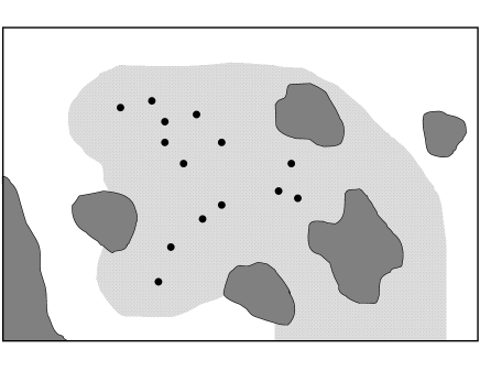
Figure 1: Schematic representation of the heterogeneous medium $\Omega$. The little black discs represent the pedestrians, while the dark gray zones are the parts where the pedestrians cannot penetrate (i.e. subsets of $\Omega_{s}$). The pedestrians are considered here to be the microscopic entities, while the grayish shadow indicates a macroscopic crowd; see Section 2.1 for the precise distinction between micro and macro made in terms of supports of micro and macro measures.

In this framework, we choose for the following working plan: Firstly, we extend the multiscale approach developed by Piccoli et al. [10] (see also the context described in [21] and [22]) to the case of counterflow of pedestrians; then we allow the pedestrian dynamics to take place in the heterogeneous domain $\Omega$, and finally, we include an implicit velocity law for the pedestrians motion. The main reason why we choose the counterflow scenario [also called bidirectional flow [7]] out of the many other well-studied crowd dynamics scenarios is at least threefold:

• Pedestrians counterflow is often encountered in the everyday life: at pedestrian traffic lights, or just observe next week-end, when you go shopping, the dynamics of people coming against your walking direction [especially if you are positioned inside narrow corridors].

• The walkers trying to move faster by avoiding local interactions with the oncoming pedestrians facilitate the occurrence of a well-known self-organized macroscopic pattern – lane formation; see, for instance [15].

• We expect the solution to microscopic models posed in narrow corridors to be computationally cheap. Consequently, extensive sensitivity analyses can be performed and the corresponding simulation results can be in principle tested against existing experimental observations [19, 8].

The presence of heterogeneities is quite natural. Pedestrians typically follow existing streets, walking paths, they trust building maps, etc. They take into account the local environment of the place where they are located. If the number of pedestrians is relatively high compared to the available walking space, then the crowd-structure interaction becomes of vital importance; see e.g. [6] for preliminary results in this direction.

As long term plan, we wish to understand what are the microscopic mechanisms behind the formation of lanes in heterogeneous environments. In other words, we aim at identifying links between social force-type microscopic models (see [14, 20], e.g.) and macroscopic models for lanes (see [15, 3], e.g.) in the presence of heterogeneities. Here we follow a measure-theoretical approach to describe the dynamics of crowds. Our working strategy is very much inspired by the works by M. Böhm [4] and Piccoli et al. [10].

The paper is organized as follows: In Section 2 we introduce basic modeling concepts defining the mass and porosity measures needed here, as well as a coupled system of transport equations for measures. In Section 3 we present our concept of social velocity. Section 4 contains the main result of our paper – the weak formulation of a micro-macro system for pedestrians moving in heterogeneous domains. We close the paper with a numerical illustration of our microscopic model (Section 5) exhibiting effects induced by an implicitly defined velocity.

2 Modeling with mass measures. The porosity measure

For basic concepts of measure theory and their interplay with modeling in materials and life science, we refer the reader, for instance, to [12] and respectively to [4, 21, 25].

2.1 Mass measure

Let $\Omega\subset\mathbb{R}^{d}$ be a domain (read: object, body) with mass. Since we have in mind physically relevant situations only, we consider $d\in\{1,2,3\}$. However, most of the considerations reported here do not depend on the choice of the space dimension $d$. Let $\mu_{m}(\Omega^{\prime})$ be defined as the mass in $\Omega^{\prime}\subset\Omega$. Note that whenever we write $\Omega^{\prime}\subset\Omega$, we actually mean that $\Omega^{\prime}$ is such that $\Omega^{\prime}\in\mathcal{B}(\Omega)$, where $\mathcal{B}(\Omega)$ the $\sigma$-algebra of the Borel subsets of $\Omega$. As a rule, we assume $\mu_{m}$ to be defined on all elements of $\mathcal{B}(\Omega)$.

In Sections 2.1.1 and 2.1.2, we consider two specific interpretations of this mass measure that we need to describe the behavior of pedestrians at two separated spatial scales.

2.1.1 Microscopic mass measure

Suppose that $\Omega$ contains a collection of $N$ point masses (each of them of mass scaled to 1), and denote their positions by $\{p_{k}\}_{k=1}^{N}\subset\Omega$, for $N\in\mathbb{N}$. We want $\mu_{m}$ to be a counting measure (see Sect. 1.2.4 in [1], e.g.) with respect to these point masses, i.e. for all $\Omega^{\prime}\in\mathcal{B}(\Omega)$:

$$\mu_{m}(\Omega^{\prime})=\#\{p_{k}\in\Omega^{\prime}\}.$$ (1)

This can be achieved by representing $\mu_{m}$ as the sum of Dirac measures, with their singularities located at the $p_{k}$, $k\in\{1,2,\ldots,N\}$, namely:

$$\mu_{m}=\sum_{k=1}^{N}\delta_{p_{k}}.$$ (2)

We refer to the measure $\mu_{m}$ defined by (2) as microscopic mass measure.

2.1.2 Macroscopic mass measure

Let us now consider another example of mass measure $\mu_{m}$. To do this, we assume that the following postulate applies to $\mu_{m}$:

Postulate 2.1 (Assumptions on $\mu_{m}$).

1. $\mu_{m}\geqslant 0$.
   

2. $\mu_{m}$ is $\sigma$-additive.
   

3. $\mu_{m}\ll\lambda^{d}$, where $\lambda^{d}$ is the Lebesgue-measure in $\mathbb{R}^{d}$.

By Postulate 2.1 (i) and (ii), we have that $\mu_{m}$ is a positive measure on $\Omega$, whereas (iii) implies that there is no mass present in a set that has no volume (w.r.t. $\lambda^{d}$). A mass measure satisfying Postulate 2.1 is in this context referred to as a macroscopic mass measure. Radon-Nikodym Theorem (see [12] for more details on this subject) guarantees the existence of a real, non-negative density $\hat{\rho}\in L_{\lambda^{d}}^{1}(\Omega)$ such that:

$$\mu_{m}(\Omega^{\prime})=\int_{\Omega^{\prime}}\hat{\rho}(x)d\lambda^{d}(x)\hskip 28.45274pt\text{for all }\Omega^{\prime}\in\mathcal{B}(\Omega).$$ (3)

Similarly, we introduce time-dependent mass measures $\mu_{t}$, where the time slice $t\in S$ enters as a parameter.

2.2 Porosity measure

Let $\Omega\subset\mathbb{R}^{d}$ be a heterogeneous domain composed of two distinct regions: free space for pedestrian motion and a matrix (obstacles) such that $\Omega=\Omega_{s}\cup\Omega_{p}$ (disjoint union), where $\Omega_{s}$ is the matrix (solid part) of $\Omega$ and $\Omega_{p}$ is the free space (pores). This notation is very much inspired by the modeling of transport and chemical reactions in porous media; see [2], e.g.

Let $\mu_{p}(\Omega^{\prime})$ be the volume of pores in $\Omega^{\prime}\subset\Omega$.

Postulate 2.2 (Assumptions on $\mu_{p}$).

1. $\mu_{p}\geqslant 0$.
   

2. $\mu_{p}$ is $\sigma$-additive.
   

3. $\mu_{p}\ll\lambda^{d}$.

By Postulate 2.2 (i) and (ii), we have that $\mu_{p}$ is a measure on $\Omega$. We refer to $\mu_{p}$ as a porosity measure (cf. [4]). The absolute continuity statement in (iii) formulates mathematically that there cannot be a non-zero volume of pores included in a set that has zero volume (w.r.t. $\lambda^{d}$). Assume that $\Omega$ is such that $\lambda^{d}(\Omega)<\infty$. Then the Radon-Nikodym Theorem ensures the existence of a function $\phi\in L^{1}_{+}(\Omega)$ such that:

$$\mu_{p}(\Omega^{\prime})=\int_{\Omega^{\prime}}\phi d\lambda^{d}\quad\mbox{ for all }\Omega^{\prime}\in\mathcal{B}(\Omega).$$ (4)

Note that $\mu_{p}(\Omega^{\prime})$ measures the volume of a subset of $\Omega^{\prime}$ (namely of $\Omega^{\prime}\cap\Omega_{p}$). So, we get that

$$\mu_{p}(\Omega^{\prime})=\lambda^{d}(\Omega^{\prime}\cap\Omega_{p})\leqslant\lambda^{d}(\Omega^{\prime})\quad\mbox{ for all }\Omega^{\prime}\in\mathcal{B}(\Omega).$$ (5)

We thus have $\int_{\Omega^{\prime}}\phi d\lambda^{d}\leqslant\int_{\Omega^{\prime}}d\lambda^{d}$, or $\int_{\Omega^{\prime}}(1-\phi)d\lambda^{d}\geqslant 0$. Since the latter inequality holds for any choice of $\Omega^{\prime}$, it follows that $\phi\leqslant 1$ almost everywhere in $\Omega$.

2.3 Transport of a measure

For the sequel, we wish to restrict the presentation to the case $d=2$. For our time interval $S$ and for each $i\in\{1,2\}$, we denote the velocity field of the corresponding measure by $v^{i}(t,x)$ with $(t,x)\in S\times\Omega$. Let also $\mu_{t}^{1}$, and $\mu_{t}^{2}$ be two time-dependent mass measures. Note that for each choice of $i$, the dependence on $t$ of $v^{i}$ is comprised in the functional dependence of $v^{i}$ on both measures $\mu_{t}^{1}$, and $\mu_{t}^{2}$. This is clearly indicated in (9). The fact that here we deal with two mass measures $\mu_{t}^{1}$ and $\mu_{t}^{2}$, transported with corresponding velocities $v^{1}$ and $v^{2}$, translates into:

$$\left\{\begin{aligned} \dfrac{\partial\mu_{t}^{1}}{\partial t}+\nabla\cdot(\mu_{t}^{1}v^{1})&=0,\\ \dfrac{\partial\mu_{t}^{2}}{\partial t}+\nabla\cdot(\mu_{t}^{2}v^{2})&=0,\end{aligned}\right.\hskip 28.45274pt\text{for all }(t,x)\in S\times\Omega.$$ (6)

These equations are accompanied by the following set of initial conditions:

$$\mu_{t}^{i}=\mu_{0}^{i}\mbox{ as }t=0\mbox{ for }i\in\{1,2\}.$$ (7)

It is worth noting that (6) is the measure-theoretical counterpart of the Reynolds Theorem in continuum mechanics. To be able to interpret what a partial differential equation in terms of measures means, we give a weak formulation of (6). Essentially, for all test functions $\psi^{1},\psi^{2}\in C_{0}^{1}(\bar{\Omega})$ and for almost every $t\in S$, the following identity holds:

$$\dfrac{d}{dt}\int_{\Omega}\psi^{i}(x)d\mu_{t}^{i}(x)=\int_{\Omega}v^{i}(t,x)\cdot\nabla\psi^{i}(x)d\mu_{t}^{i}(x)\mbox{ for all }i\in\{1,2\}.$$ (8)

Definition 2.1 (Weak solution of (6)).

The pair $(\{\mu_{t}^{1}\}_{t\geqslant 0},\{\mu_{t}^{2}\}_{t\geqslant 0})$ is called a weak solution of (6), if for all $i\in\{1,2\}$ the following properties hold:

1. the mappings $t\mapsto\int_{\Omega}\psi^{i}(x)d\mu_{t}^{i}(x)$ are absolutely continuous for all $\psi^{i}\in C_{0}^{1}(\bar{\Omega})$;

2. $v^{i}\in L^{2}\Bigl{(}S;L_{\mu_{t}^{i}}^{1}(\Omega)\Bigr{)}$;

3. Equation (8) is fulfilled.

We refer the reader to [9] for an example where the existence of weak solutions to a similar (but easier) transport equation for measures has been rigorously shown.

3 Social velocities

We follow very much the philosophy developed by Helbing, Vicsek and coauthors (see, e.g. [15] and references cited therein) which defends the idea that the pedestrian’s motion is driven by a social force. Is worth noting that similar thoughts were given in this direction (motion of social masses/networks) much earlier, for instance, by Spiru Haret [13] and Antonio Portuondo y Barceló [23]. Moreover, other authors (for instance, Hoogendoorn and Bovy [16]) prefer to account also for the Zipfian principle of least effort for the human behavior. We do not attempt to capture the least effort principle in this study.

3.1 Specification of the velocity fields $v^{i}$

Until now, we have not explicitly defined the velocity fields $v^{i}$ ($i\in\{1,2\}$). Very much inspired by the social force model by Dirk Helbing et al. [14], the velocity of a pedestrian is modeled as a desired velocity $v_{\text{des}}^{i}$ perturbed by a component $v_{[\mu_{t}^{1},\mu_{t}^{2}]}^{i}$. The latter component is due to the presence of other individuals, both from the pedestrian’s own subpopulation and from the other subpopulation. The desired velocity is independent of the measures $\mu_{t}^{1}$ and $\mu_{t}^{2}$, and represents the velocity that an agent would have had in absence of other pedestrians.

For each $i\in\{1,2\}$, the velocity $v^{i}$ is defined by superposing the two velocities $v_{\text{des}}^{i}$ and $v_{[\mu_{t}^{1},\mu_{t}^{2}]}^{i}$ as follows:

$$v^{i}(t,x):=v_{\text{des}}^{i}(x)+v_{[\mu_{t}^{1},\mu_{t}^{2}]}^{i}(x),\hskip 28.45274pt\text{for all }t\in(0,T)\text{ and }x\in\Omega.$$ (9)

For a counterflow scenario, the desired velocities of the two subpopulations follow opposite directions. We thus take

$$v_{\text{des}}^{i}(x)=v_{\text{des}}^{i}\in\mathbb{R}^{2}$$

fixed (for $i\in\{1,2\}$) and

$$v_{\text{des}}^{1}=-v_{\text{des}}^{2}.$$

The component $v_{[\mu_{t}^{1},\mu_{t}^{2}]}^{i}$ models the effect of interactions with other pedestrians on the current velocity. Since the interactions between members of the same subpopulation differ (in general) from the interactions between members of opposite subpopulations, we assume that $v_{[\mu_{t}^{1},\mu_{t}^{2}]}^{i}$ consists of two parts:

$$v_{[\mu_{t}^{1},\mu_{t}^{2}]}^{i}(x) := \int_{\Omega\setminus\{x\}}f^{\text{own}}(|y-x|)g(\alpha_{xy}^{i})\dfrac{y-x}{|y-x|}d\mu_{t}^{i}(y)$$ (10)

$$+\int_{\Omega\setminus\{x\}}f^{\text{opp}}(|y-x|)g(\alpha_{xy}^{i})\dfrac{y-x}{|y-x|}d\mu_{t}^{j}(y),$$

for $i\in\{1,2\}$, where $j=1$ if $i=2$ and vice versa. In (10) we have used the following:

• $f^{\text{own}}$ and $f^{\text{opp}}$ are continuous functions from $\mathbb{R}_{+}$ to $\mathbb{R}$, describing the effect of the mutual distance between individuals on their interaction. Compare the concept of distance interactions defined in [25]. $f^{\text{own}}$ incorporates the influence by members of the same subpopulation, whereas $f^{\text{opp}}$ accounts for the interaction between members of opposite subpopulations. $f^{\text{own}}$ is a composition of two effects: on the one hand individuals are repelled, since they want to avoid collisions and congestion, on the other hand they are attracted to other group mates, in order not to get separated from the group. $f^{\text{opp}}$ only contains a repulsive part, since we assume that pedestrians do not want to stick to the other subpopulation.

• $\alpha_{xy}^{i}$ denotes the angle between $y-x$ and $v_{\text{des}}^{i}(x)$: the angle under which $x$ sees $y$ if it were moving in the direction of $v_{\text{des}}^{i}(x)$.

• $g$ is a function from $[-\pi,\pi]$ to $[0,1]$ that encodes the fact that an individual’s vision is not equal in all directions.

Regarding the specific choice of $f^{\text{own}}$, $f^{\text{opp}}$ and $g$ we are very much inspired by [14] and [10], e.g. However we do not use exactly their way of modeling pedestrians’ interaction forces. We list here the following forms for the functions $f^{\text{own}}$, $f^{\text{opp}}$ and $g$ that match the given characterization:

$$f^{\text{opp}}(s) := \left\{\begin{array}[]{ll}-F^{\text{opp}}\Bigl{(}\dfrac{1}{s^{2}}-\dfrac{1}{(R_{r}^{\text{opp}})^{2}}\Bigr{)},&\mbox{if $s\leqslant R_{r}^{\text{opp}}$;}\\ 0,&\mbox{if $s>R_{r}^{\text{opp}}$,}\end{array}\right.$$ (13)

$$f^{\text{own}}(s) := \left\{\begin{array}[]{ll}-F^{\text{own}}\Bigl{(}\dfrac{1}{s}-\dfrac{1}{R_{r}^{\text{own}}}\Bigr{)}\Bigl{(}\dfrac{1}{s}-\dfrac{1}{R_{a}^{\text{own}}}\Bigr{)},&\mbox{if $s\leqslant R_{a}^{\text{own}}$;}\\ 0,&\mbox{if $s>R_{a}^{\text{own}}$,}\end{array}\right.$$ (16)

$$g(\alpha) := \sigma+(1-\sigma)\dfrac{1+\cos(\alpha)}{2},\hskip 28.45274pt\text{for }\alpha\in[-\pi.\pi].$$ (17)

Here $F^{\text{opp}}$ and $F^{\text{own}}$ are fixed, positive constants. The constants $R_{r}^{\text{opp}}$, $R_{r}^{\text{own}}$ (radii of repulsion) and $R_{a}^{\text{own}}$ (radius of attraction) are fixed and should be chosen such that $0<R_{r}^{\text{own}}<R_{a}^{\text{own}}$ and $0<R_{r}^{\text{opp}}$. Furthermore, the restriction $\max\{R_{a}^{\text{own}},R_{r}^{\text{opp}}\}\ll L$ has to be fulfilled. The interaction $f^{\text{opp}}$ is designed such that individuals “feel” repulsion (i.e. $f^{\text{opp}}<0$) from another pedestrian if they are placed within a distance $R_{r}^{\text{opp}}$ from one another. The corresponding statement holds for $f^{\text{own}}$ if individuals are within the distance $R_{r}^{\text{own}}$. Additionally, an individual is attracted to a second individual if their mutual distance ranges between $R_{r}^{\text{own}}$ and $R_{a}^{\text{own}}$.
The function $g$ ensures that an individual experiences the strongest influence from someone straight ahead, since $g(0)=1$ for any $\sigma\in[0,1]$. The constant $\sigma$ is a tuning parameter called potential of anisotropism. It determines how strongly a pedestrian is focussed on what happens in front of him, and how large the influence is of people at his sides or behind him.

In the remainder of this section, we suggest four different alternatives for the definition of $v_{[\mu_{t}^{1},\mu_{t}^{2}]}^{i}$ by indicating various special choices of distance interactions and visibility angles (conceptually similar to $\alpha_{xy}^{i}$) as they arise in (10). All of them boil down to including an implicit dependency of the actual velocity $v^{i}=v_{\text{des}}^{i}+v_{[\mu_{t}^{1},\mu_{t}^{2}]}^{i}$. Note that this effect increases the degree of realism of the model, but on the other hand it makes the mathematical justification of the corresponding models much harder to get.

3.1.1 Modification of the angle $\alpha_{xy}^{i}$

We defined the angle $\alpha_{xy}^{i}$ as the angle between the vector $y-x$ and $v_{\text{des}}^{i}(x)$. However this is not a good definition if the pedestrian in position $x$ is not moving in the direction of $v_{\text{des}}^{i}(x)$ (or, in a broader sense, if the actual speed cannot be approximated sufficiently well by the desired velocity). Therefore we suggest to define $\alpha_{xy}^{i}=\alpha_{xy}^{i}(t)$ as the angle between $y-x$ and $v^{i}(t,x)$.

3.1.2 Prediction of mutual distance in (near) future

Up to now the functions $f^{\text{own}}$ and $f^{\text{opp}}$ depended on the actual distance between $x$ and $y$ at time $t$. However pedestrians are likely to anticipate on the distance they expect to have after a certain (small) time-step (say, some fixed $\Delta t\in\mathbb{R}$). In practice, this means that at a time $t\in S$ a person will modify his velocity (either in direction, or in magnitude, or both) if he foresees a collision at time $t+\Delta t\in S$.

To predict the mutual distance between $x$ and $y$ at time $t+\Delta t$, the current velocities at $x$ and $y$ are used for extrapolation. The predicted distance is: $|(y+v(y,t)\Delta t)-(x+v(x,t)\Delta t)|$. Consequently, sticking to the notation in (10), the interaction potential $f^{\text{own}}$ and $f^{\text{opp}}$ should depend on $|(y+v^{i}(t,y)\Delta t)-(x+v^{i}(t,x)\Delta t)|$ and on $|(y+v^{j}(t,y)\Delta t)-(x+v^{i}(t,x)\Delta t)|$ respectively (where $j=1$ if $i=2$ and vice versa).

3.1.3 Prediction of mutual distance within a time interval in the (near) future

The disadvantage of using $|(y+v(y,t)\Delta t)-(x+v(x,t)\Delta t)|$ is that $\Delta t$ is fixed. A pedestrian can thus only predict the distance at an a priori specified point in time in the future. However, people are able to anticipate also if they expect a collision to occur at a time that is not equal to $t+\Delta t$. We assume now that we are given a fixed $\Delta t_{\text{max}}\in\mathbb{R}_{+}$ such that an individual can predict mutual distances by extrapolation for any time $\tau\in(t,t+\Delta t_{\text{max}})$. Thus, $\Delta t_{\text{max}}$ imposes a bound on how far can an individual look ahead into the future. To capture this effect, we suggest to replace $f^{\text{own}}(|y-x|)$ and $f^{\text{opp}}(|y-x|)$ by:

$$\frac{1}{\Delta t_{\text{max}}}\int_{0}^{\Delta t_{\text{max}}}f^{\text{own}}(\big{|}(y+v^{i}(t,y)\tau)-(x+v^{i}(t,x)\tau)\big{|})d\tau,$$ (18)

and

$$\frac{1}{\Delta t_{\text{max}}}\int_{0}^{\Delta t_{\text{max}}}f^{\text{opp}}(\big{|}(y+v^{j}(t,y)\tau)-(x+v^{i}(t,x)\tau)\big{|})d\tau,$$ (19)

respectively.

3.1.4 Weighted prediction

Since an individual probably attaches more value to his predictions for points in time that are nearer by than others, one additional modification comes to our mind. Let $h:[t,t+\Delta t_{\text{max}}]\rightarrow[0,1]$ be a weight function. Then instead of (18) and (19), we propose

$$\frac{1}{\Delta t_{\text{max}}}\int_{0}^{\Delta t_{\text{max}}}f^{\text{own}}(\big{|}(y+v^{i}(t,y)\tau)-(x+v^{i}(t,x)\tau)\big{|})h(\tau)d\tau,$$ (20)

and

$$\frac{1}{\Delta t_{\text{max}}}\int_{0}^{\Delta t_{\text{max}}}f^{\text{opp}}(\big{|}(y+v^{j}(t,y)\tau)-(x+v^{i}(t,x)\tau)\big{|})h(\tau)d\tau.$$ (21)

If $h$ is decreasing, then the influence of $t_{1}$ is larger than the influence of $t_{2}$, if $t_{1}<t_{2}$ (which matches our intuition).

3.2 Two-scale measures

We now consider the explicit decomposition of the measures $\mu_{t}^{1}$ and $\mu_{t}^{2}$. Let the pair $(\theta_{1},\theta_{2})$ be in $[0,1]^{2}$, and consider the following decomposition of $\mu_{t}^{1}$ and $\mu_{t}^{2}$:

$$\mu_{t}^{i}=\theta_{i}m_{t}^{i}+(1-\theta_{i})M_{t}^{i},\hskip 28.45274pti\in\{1,2\}.$$ (22)

Here, $m_{t}^{i}$ is a microscopic measure. We consider $\{p_{k}^{i}(t)\}_{k=1}^{N^{i}}\subset\Omega$ to be the positions at time $t$ of $N^{i}$ chosen pedestrians, that are members of subpopulation $i$. We want $m_{t}^{i}$ to be a counting measure with respect to these pedestrians, i.e. for all $\Omega^{\prime}\in\mathcal{B}(\Omega)$:

$$m_{t}^{i}(\Omega^{\prime})=\#\{p_{k}^{i}(t)\in\Omega^{\prime}\},\hskip 28.45274pti\in\{1,2\}.$$ (23)

We thus define $m_{t}^{i}$ as the sum of Dirac masses (cf. Section 2.1.1), centered at the $p_{k}^{i}$, $k=1,2,\ldots,N^{i}$:

$$m_{t}^{i}=\sum_{k=1}^{N^{i}}\delta_{p_{k}^{i}(t)},\hskip 28.45274pti\in\{1,2\}.$$ (24)

$M_{t}^{i}$ is the macroscopic part of the measure, which takes into account the part of the crowd that is considered continuous. We consequently have $M_{t}^{i}\ll\lambda^{2}$, since a set of zero volume cannot contain any mass. Note that we are thus in the setting of Section 2.1.2. Now, Radon-Nikodym Theorem guarantees the existence of a real, non-negative density $\hat{\rho}^{i}(t,\cdot)\in L_{\lambda^{2}}^{1}(\Omega)$ such that:

$$M_{t}^{i}(\Omega^{\prime})=\int_{\Omega^{\prime}}\hat{\rho}^{i}(t,x)d\lambda^{2}(x)$$ (25)

for all $\Omega^{\prime}\in\mathcal{B}(\Omega)$ and all $i\in\{1,2\}$.

4 Micro-macro modeling of pedestrians motion in heterogeneous domains

We have already made clear that we want to model the heterogeneity of the interior of the corridor. In practice this means that pedestrians cannot enter all parts of the domain. As described in Section 2.2, we have a measure $\mu_{p}$ corresponding to the porosity of the domain (which is fixed in time). However, we note that the concept of porosity (cf. Section 2.2) is a macroscopic one. For this reason only the macroscopic part of the mass measure in (22) needs some modification with respect to the porosity. In this context, one should be aware of the analogy with mathematical homogenization. This technique distinguishes between microscopic and macroscopic scales, where we also see that some (averaged) characteristics are only defined on the macroscopic scale. For more details, the reader is referred to [2] or [17]. In $\mathbb{R}^{2}$, we have $\mu_{p}\ll\lambda^{2}$. Furthermore $M_{t}^{i}\ll\mu_{p}$ for $i\in\{1,2\}$ and a.e. $t\in S$. This is obvious, since no pedestrians can be present in a set that has no pore space (i.e. zero porosity measure). A basic property of Radon-Nikodym derivatives now gives us:

$$\dfrac{dM_{t}^{i}}{d\lambda^{2}}=\dfrac{dM_{t}^{i}}{d\mu_{p}}\dfrac{d\mu_{p}}{d\lambda^{2}}\quad i\in\{1,2\}\text{ for almost every }t\in S.$$ (26)

We have already defined $\hat{\rho}^{i}(t,\cdot):=\dfrac{dM_{t}^{i}}{d\lambda^{2}}$ and $\phi:=\dfrac{d\mu_{p}}{d\lambda^{2}}$. If we now denote by $\rho^{i}(t,\cdot)$ the Radon-Nikodym derivative $\dfrac{dM_{t}^{i}}{d\mu_{p}}$, the following relation holds: $\hat{\rho}^{i}(t,\cdot)\equiv\rho^{i}(t,\cdot)\phi(\cdot)$ for all $i\in\{1,2\}$.

4.1 Weak formulation for micro-macro mass measures

We now have the following measure:

$$\mu_{t}^{i}=\theta_{i}m_{t}^{i}+(1-\theta_{i})M_{t}^{i},\hskip 28.45274pti\in\{1,2\},$$ (27)

as was given in (22), where now:

$$m_{t}^{i}=\sum_{k=1}^{N^{i}}\delta_{p_{k}^{i}(t)},\hskip 28.45274ptdM_{t}^{i}(x)=\rho^{i}(t,x)\phi(x)d\lambda^{2}(x).$$ (28)

This specific form of the measure will now be included in the weak formulation (8), with velocity field (9)-(10). The real positive numbers $\theta_{i}$ ($i\in\{1,2\}$) are intrinsic scaling parameters depending on $N^{i}$.

The transport equation (8) takes the following form:

$$\dfrac{d}{dt}\Bigl{(}\theta_{i}\sum_{k=1}^{N^{i}}\psi^{i}\bigl{(}p_{k}^{i}(t)\bigr{)}+(1-\theta_{i})\int_{\Omega}\psi^{i}(x)\rho^{i}(t,x)\phi(x)d\lambda^{2}(x)\Bigr{)}=$$

$$\theta_{i}\sum_{k=1}^{N^{i}}v^{i}\bigl{(}t,p_{k}^{i}(t)\bigr{)}\cdot\nabla\psi^{i}\bigl{(}p_{k}^{i}(t)\bigr{)}+(1-\theta_{i})\int_{\Omega}v^{i}(t,x)\cdot\nabla\psi^{i}(x)\rho^{i}(t,x)\phi(x)d\lambda^{2}(x),$$ (29)

for all $i\in\{1,2\}$. Here we have used the sifting property of the Dirac distribution. In the same manner, we specify $v_{[\mu_{t}^{1},\mu_{t}^{2}]}^{i}$ from (10) as

$$v_{[\mu_{t}^{1},\mu_{t}^{2}]}^{i}(x) = \theta_{i}\sum_{\begin{subarray}{c}k=1\\ p_{k}^{i}(t)\neq x\end{subarray}}^{N^{i}}f^{\text{own}}(|p_{k}^{i}(t)-x|)g(\alpha_{xp_{k}^{i}(t)}^{i})\dfrac{p_{k}^{i}(t)-x}{|p_{k}^{i}(t)-x|}$$

$$+(1-\theta_{i})\int_{\Omega}f^{\text{own}}(|y-x|)g(\alpha_{xy}^{i})\dfrac{y-x}{|y-x|}\rho^{i}(t,y)\phi(y)d\lambda^{2}(y)$$

$$+\theta_{j}\sum_{\begin{subarray}{c}k=1\\ p_{k}^{j}(t)\neq x\end{subarray}}^{N^{j}}f^{\text{opp}}(|p_{k}^{j}(t)-x|)g(\alpha_{xp_{k}^{j}(t)}^{i})\dfrac{p_{k}^{j}(t)-x}{|p_{k}^{j}(t)-x|}$$

$$+(1-\theta_{j})\int_{\Omega}f^{\text{opp}}(|y-x|)g(\alpha_{xy}^{i})\dfrac{y-x}{|y-x|}\rho^{j}(t,y)\phi(y)d\lambda^{2}(y),$$

for $i\in\{1,2\}$, and $j$ as before ($j=1$ if $i=2$ and vice versa). We have omitted the exclusion of $\{x\}$ from the domain of integration (in the macroscopic part), since $\{x\}$ is a nullset and thus negligible w.r.t. $\lambda^{2}$. Note that the sums may be evaluated in any point $x\in\Omega$ (not necessarily $x=p_{k}^{i}(t)$ for some $i$ and $k$); the integral parts may also be evaluated in all $x$, including $x=p_{k}^{i}(t)$ for some $i$ and $k$.

5 Numerical illustration

We wish to illustrate now the microscale description of a counterflow scenario (i.e. for $\theta_{1}=\theta_{2}=1$) by presenting plots of the configuration of all individuals situated in a given corridor at specific moments in time.

We consider a specific instance in which there are in total 40 individuals (20 in each subpopulation). The dimensions of the corridor are $d=4$ and $L=20$. The velocity is taken as defined in (10)-(17). Furthermore, the following model parameters are used: $v_{\text{des}}^{1}=1.34e_{1}$, $v_{\text{des}}^{2}=-1.34e_{1}$, $F^{\text{opp}}=0.3$, $F^{\text{own}}=0.3,$ $R_{r}^{\text{opp}}=2,$ $R_{a}^{\text{own}}=2,$ $R_{r}^{\text{own}}=0.5$, $F^{\text{w}}=0.5$, $R^{\text{w}}=0.5,$ $\sigma=0.5.$

In Figure 2, we show the configuration in the corridor at times $t=0$, $t=7.5$, and $t=15$. The individuals of the subpopulation 1 are colored blue, while the individuals of the subpopulation 2 are colored red. Clearly, self-organization can be observed in the system: Pedestrians that desire to move in the same direction form lanes (in this case, three of them). This feature is observed and described extensively in literature, cf. e.g. [15].

Another feature, pointed out by Figure 2, is the following: Within the three already formed lanes, small clusters of people are formed. This flocking is a result of the typical choice for $f^{\text{own}}$ in (16). Members of the same subpopulation are repelled if their mutual distance is in the range $(0,R_{r}^{\text{own}})$; they are attracted if their mutual distance is in the range $(R_{r}^{\text{own}},R_{a}^{\text{own}})$. No interaction takes place if individuals are more than a distance $R_{a}^{\text{own}}$ apart.

The attraction part of the interaction causes individuals that are already relatively close to get even closer, until they are at a distance $R_{r}^{\text{own}}$. For distances around $R_{r}^{\text{own}}$, there is an interplay between repulsion and attraction, eventually leading to some equilibrium in the mutual distances between neighboring individuals in one cluster. In Figure 2, we observe self-organized patterns even within clusters.

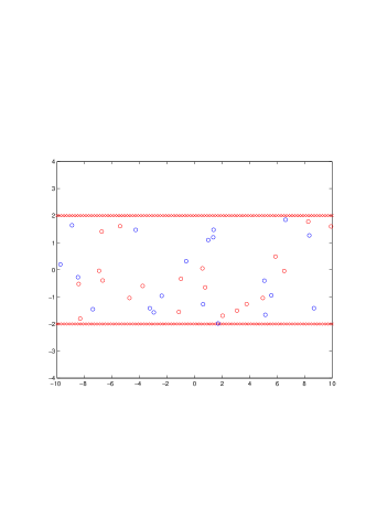
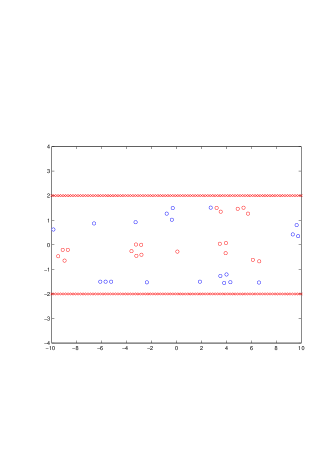
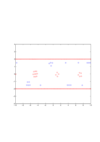
Figure 2: The simulation of a crowd’s motion in a corridor of length $L=20$ and width $d=4$. Each of the two sub-populations consists of 20 individuals. The images were taken at $t=0$ (left), $t=7.5$ (middle), $t=15$ (right).

References

- [1] R. B. Ash. Measure, Integration, and Functional Analysis. Academic Press, London, 1972.
- [2] J. Bear. Dynamics of Fluids in Porous Media. Dover New York, 1988.
- [3] N. Bellomo and C. Dogbe. On the modelling crowd dynamics from scaling to hyperbolic macroscopic models. Math. Models Methods Appl. Sci., 18(2008):1317–1345, 2008.
- [4] M. Böhm. Lecture Notes in Mathematical Modeling. 2006. Department of Mathematics, University of Bremen.
- [5] R. C. Bradley. An elementary treatment of the Radon-Nikodym derivative. The American Mathematical Monthly, 96(Vol. 5):pp. 437–440, 1989.
- [6] L. Bruno, A. Tosin, P. tricerri, and F. Venuti. Non-local first-oder modelling of crowd dynamics: a multidimensional framework with applications. 2010. arxiv.org/pdf/1003.3891.
- [7] M. Campanella, S. Hoogendoorn, and W. Daamen. Calibration of pedestrian models with respect to lane formation self-organisation. Technical report, Department of Transport and Planning, Delft University of Technology, 2008.
- [8] M. Campanella, S. Hoogendoorn, and W. Daamen. The effects of heterogeneity on self-organized pedestrian flows. J. Transp. Res. Board, 2124:148–156, 2009.
- [9] C. Canuto, F. Fagnani, and P. Tilli. A Eulerian approach to the analysis of rendez-vous algorithms. In Proceedings of the 17th IFAC World Congress (IFAC’08), pages pp. 9039–9044. IFAC World Congress, Seoul, Korea, July 2008.
- [10] E. Cristiani, B. Piccoli, and A. Tosin. Multiscale modeling of granular flows with application to crowd dynamics. 2010.
- [11] A. F. Filippov. Differential Equations with Discontinuous Righthand Sides. Mathematics and Its Applications. Kluwer, Dordrecht, 1988.
- [12] P. R. Halmos. Measure Theory. D. van Nostrand, Princeton, New Jersey, 1956.
- [13] S. Haret. Mécanique sociale. Gauthier-Villars, Paris, 1910.
- [14] D. Helbing and P. Molnár. Social force model for pedestrian dynamics. Physical Review E, 51(5):pp. 4282–4286, 1995.
- [15] D. Helbing and T. Vicsek. Optimal self-organization. New Journal of Physics, 1:pp. 13.1–13.17, 1999.
- [16] S. Hoogendoorn and P. H. L. Bovy. Simulation of pedestrian flows by optimal control and differential games. Optim. Control Appl. Meth., 24:153–172, 2003.
- [17] V. Jikov, S. Kozlov, and O. Oleinik. Homogenization of Differential Operators and Integral Functionals. Springer-Verlag, 1994. (translated from the Russian by G.A. Yosifian).
- [18] C. Kipnis and C. Landim. Scaling Limits of Interacting Particle Systems. Springer Verlag, 1998.
- [19] T. Kretz, A. Grünebohm, M. Kaufman, F. Mazur, and M. Schreckenberg. Experimental study of pedestrian counterflow in a corridor. Journal of Statistical Mechanics: Theory and Experiment, P10001:pp. 1–18, 2006.
- [20] B. Maury, A. Roudneff-Chupin, and F. Santambrogio. A macroscopic crowd motion model of gradient flow type. Mathematical Models and Methods in Applied Sciences, 2010. (accepted).
- [21] B. Piccoli and A. Tosin. Pedestrian flows in bounded domains with obstacles. Continuum Mech Thermodyn., 21:pp. 85–107, 2009.
- [22] B. Piccoli and A. Tosin. Time-evolving measures and macroscopic modeling of pedestrian flow. Arch. Ration. Mech. Anal., 2010. (DOI) 10.1007/s00205-010-0366-y.
- [23] A. Portuondo y Barceló. Apuntes sobre Mecánica Social. Establecimiento Topográfico Editorial, Madrid, 1912.
- [24] A. Schadschneider. I am a football fan … get me out of here. Physics World, pages 21–25, July 2010.
- [25] F. Schuricht. Interactions in continuum physics. mathematical modelling of bodies with complicated bulk and boundary behavior. Quad. Mat., Dept. Seconda Univ. Napoli, Caserta, 20:169 – 196, 2007.
- [26] T. Vicsek. A question of scale. Nature, 411:421, 2001.