Abundance determination in H II regions from spectra without the [O II]$\lambda$3727+$\lambda$3729 line

Abstract

We suggest an empirical calibration for determination of oxygen and nitrogen abundances and electron temperature in H ii regions where the [O ii]$\lambda$3727+$\lambda$3729 line ($R_{2}$) is not available. The calibration is based on the strong emission lines of O⁺⁺, N⁺, and S⁺ (NS calibration) and derived using the spectra of H ii regions with measured electron temperatures as calibration datapoints. The NS calibration makes it possible to derive abundances for H ii regions in nearby galaxies from the SDSS spectra where $R_{2}$ line is out of the measured wavelength range, but can also be used for the oxygen and nitrogen abundances determinations in any H ii region independently whether the nebular oxygen line [O ii]$\lambda$3727+$\lambda$3729 is available or not. The NS calibration provides reliable oxygen and nitrogen abundances for H ii regions over the whole range of metallicities.

1 Introduction

The Sloan Digital Sky Survey (SDSS) (York et al., 2000) provides a very large database of spectra of individual H ii regions in nearby galaxies and global emission-line spectra of distant galaxies. The wavelength range of the SDSS spectra is 3800 – 9300Å so that for nearby galaxies with redshift $z$ $\la$ 0.023, the [O ii]$\lambda$3727+$\lambda$3729 emission line is out of that range. The absence of this line prevents the use of the standard $T_{e}$ method where the [O ii]$\lambda$3727+$\lambda$3729 line is used for the determination of the contribution of ion O⁺ to the total oxygen abundance in H ii region. Since the calibrated relations between metallicity and the relative fluxes of strong oxygen lines usually involve the [O ii]$\lambda$3727+$\lambda$3729 line, the absence of this line prevents the use of such relations to determine abundances.

Kniazev et al. (2004) have suggested that this problem can be avoided by using a modification of the standard $T_{e}$ method, based on the intensity of the auroral line [O ii]$\lambda$7320+$\lambda$7330 instead of the intensity of the [O ii]$\lambda$3727+$\lambda$3729 nebular line. This modification of the standard $T_{e}$ method was used also by Magrini et al. (2007) for abundance determinations in H ii regions in the disk of the nearby spiral galaxy M 33. Another way to overcome this problem has been suggested by Pilyugin & Thuan (2007) based on the relation, called the $ff$-relation, between the auroral and nebular oxygen line fluxes (Pilyugin et al., 2006). Using the $ff$-relation, the nebular [O ii]$\lambda$3727+$\lambda$3729 oxygen line flux can be estimated from the measured auroral [O iii]$\lambda$4363 and nebular [O iii]$\lambda$4959+$\lambda$5007 oxygen line fluxes. However, both these methods are useful only if the auroral [O iii]$\lambda$4363 oxygen line is detected in the SDSS spectra, which is not the case for the majority objects.

Pioneering work by Pagel et al. (1979) and Alloin et al. (1979) gave a method for deriving abundances in H ii regions in cases where direct measurement of the electron temperature is not possible. They suggested that the locations of H ii regions in some emission-line diagrams can be calibrated in terms of their oxygen abundances. This approach to abundance determination in H ii regions, usually referred to as the “strong line method” has been widely used. Numerous relations have been proposed to convert different emission-line ratios into metallicity or temperature estimates (e.g. Dopita & Evans, 1986; Vílchez & Esteban, 1996; Pilyugin, 2000, 2001; Pettini & Pagel, 2004; Tremonti et al., 2004; Pilyugin & Thuan, 2005; Liang et al., 2006; Stasińska, 2006; Thuan et al., 2010). Comparisons between abundances derived from various calibrations are given in the recent papers of Kewley & Ellison (2008); López-Sánchez & Esteban (2010). It was found that the calibrations based on the strong nitrogen line provide acceptable results for objects with 12+log(O/H)$\ga$8.0 only (Pérez-Montero & Contini, 2009; López-Sánchez & Esteban, 2010).

It has been argued that the ratio of the nebular nitrogen line [N ii]$\lambda$6548+$\lambda$6584 flux to the nebular oxygen line [O ii]$\lambda$3727+$\lambda$3729 flux and the ratio of the nebular sulfur line [S ii]$\lambda$6717+$\lambda$6731 flux to the nebular oxygen line [O ii]$\lambda$3727+$\lambda$3729 flux can be used as a surrogate indicators of the electron temperature and the metallicity (Pilyugin et al., 2009, 2010). Based on this, a new improved empirical calibration for the determination of electron temperatures and oxygen and nitrogen abundances in H ii regions from the strong emission lines of O⁺⁺, O⁺, N⁺ and S⁺ has recently been suggested (Pilyugin et al., 2010). This calibration provides reliable abundances for H ii regions over the whole range of metallicity. However, the calibration relations involve the nebular oxygen line [O ii]$\lambda$3727+$\lambda$3729.

From a general point of view, one may expect the ratio of the nebular nitrogen line [N ii]$\lambda$6548+$\lambda$6584 flux to the nebular sulfur line [S ii]$\lambda$6717+$\lambda$6731 flux to be useful as a surrogate indicator of the electron temperature and the metallicity in H ii region. If this is the case, then one can construct a calibration for the determination of abundances in H ii regions such that the calibration relations will not involve the line [O ii]$\lambda$3727+$\lambda$3729. This is the main objective of our study and we will follow the strategy suggested by Pilyugin et al. (2010).

Throughout the paper, we will be using the following notations for the line fluxes,

$$R_{2}=[{\rm O}\,\textsc{ii}]\lambda 3727+\lambda 3729=I_{\rm[OII]\lambda 3727+\lambda 3729}/I_{{\rm H}\beta},$$ (1)

$$N_{2}=[{\rm N}\,\textsc{ii}]\lambda 6548+\lambda 6584=I_{\rm[NII]\lambda 6548+\lambda 6584}/I_{{\rm H}\beta},$$ (2)

$$S_{2}=[{\rm S}\,\textsc{ii}]\lambda 6717+\lambda 6731=I_{\rm[SII]\lambda 6717+\lambda 6731}/I_{{\rm H}\beta},$$ (3)

$$R_{3}=[{\rm O}\,\textsc{iii}]\lambda 4959+\lambda 5007=I_{{\rm[OIII]}\lambda 4959+\lambda 5007}/I_{{\rm H}\beta}.$$ (4)

$$R_{23}=R_{2}+R_{3}.$$ (5)

The electron temperatures $t$ are given in units of 10⁴K. Furthermore, we will be using the following terminology. We refer to a ’method’ as the basic principle for deriving an abundance, e.g., $T_{\rm e}$-method, strong line method. ’Calibration’ refers to a specific form of the strong line method, e.g., the R23, N2 or NS-calibration. We also refer to ’relations’ as the resultant expressions for determination of, e.g., $t$ or O/H.

2 The NS-calibration

Here we search for a calibration based on the strong emission lines of O⁺⁺, N⁺, and S⁺. Since the ratio of the nebular nitrogen line [N ii]$\lambda$6548+$\lambda$6584 flux to the nebular sulfur line [S ii]$\lambda$6717+$\lambda$6731 flux will be used as a surrogate indicator for electron temperature and metallicity, the sought calibration will be referred to as the NS-calibration.

For the calibration, we have used a sample of 118 H ii regions with metallicities spanning a large range from Pilyugin et al. (2010). In previous study it was found that none of the considered emission line fluxes and flux ratios display a monotonic behavior with electron temperature and oxygen and nitrogen abundances over the whole temperature (or metallicity) range (Pilyugin et al., 2010). Instead, the curves show bends and it is therefore preferable to construct relations for electron temperatures and abundances for three distinct regimes.

Figure 1: The oxygen abundance (O/H)_NS (upper panel), nitrogen abundance (N/H)_NS (middle panel), and electron temperature $t_{\rm 2,NS}$ (lower panel) derived using the NS-calibration against the measured $T_{\rm e}$-method values. The open circles show the calibration H ii regions, while the line shows the case of equal values.

The following simple expression is adopted to relate the oxygen abundance to the strong line fluxes,

$$12+\log{\rm(O/H)}=a_{0}+a_{1}\,\log R_{3}+a_{2}\,\log N_{2}+a_{3}\,\log(N_{2}/S_{2}).$$ (6)

In cool high-metallicity H ii regions, the $N_{2}$ line fluxes remain approximately constant with temperature, forming a sort of plateau (Pilyugin et al., 2010). Therefore, we use log$S_{2}$ instead of log$N_{2}$ for cool high-metallicity (with log$N_{2}$$>$–0.1) H ii regions. The numerical values of the coefficients in Eq.(6) can be derived requiring that the scatter of the residuals $\sigma_{\rm O/H}$, defined as

$$\sigma_{\rm O/H}=\sqrt{\frac{1}{n}\sum\limits_{j=1}^{j=n}(\log{\rm(O/H)}_{j}^{CAL}-\log{\rm(O/H)}_{j}^{OBS})^{2}},$$ (7)

is to be minimised. In the equation above, (O/H)${}_{j}^{CAL}$ is the oxygen abundance calculated from Eq.(6) and (O/H)${}_{j}^{OBS}$ is the measured $T_{\rm e}$-based oxygen abundance.

We derive the following relations for determination of the oxygen abundance $Z_{\rm O}$=12+log(O/H)_NS

$$\begin{array}[]{lll}Z_{\rm O}&=&8.454-0.216\,\log R_{3}-0.362\,\log S_{2}-\\ &&0.101\,\log(N_{2}/S_{2}),\\ &&{\rm for}\quad\log N_{2}>-0.1\\ &&\\ Z_{\rm O}&=&8.456+0.082\,\log R_{3}+0.391\,\log N_{2}+\\ &&0.290\,\log(N_{2}/S_{2}),\\ &&{\rm for}\quad\log N_{2}<-0.1,\;\log(N_{2}/S_{2})>-0.25\\ &&\\ Z_{\rm O}&=&7.881+0.929\,\log R_{3}+0.650\,\log N_{2}+\\ &&0.025\,\log(N_{2}/S_{2}),\\ &&{\rm for}\quad\log N_{2}<-0.1,\;\log(N_{2}/S_{2})<-0.25.\\ \end{array}$$ (19)

A few datapoints deviate significantly ($>$0.3 dex) from the general trend. These were excluded in the derivation of the final calibration relations, in order to avoid any bias. The upper panel of Fig. 1 shows the oxygen abundance 12+log(O/H)_NS derived using the NS-calibration against the $T_{\rm e}$-based oxygen abundance 12+log(O/H)${}_{\rm T_{e}}$. The open circles show the calibration H ii regions. The line shows the case of equal values. Fig. 1 shows that the derived NS-calibration provides reliable oxygen abundances in H ii regions with only a few exceptions. The scatter of the residuals is $\sigma_{\rm O/H}$ = 0.077, excluding the two points with largest deviations.

In the same way, a relation for nitrogen abundance determination in H ii regions has been constructed. The relations for nitrogen abundances $Z_{\rm N}$=12+log(O/H)_NS are

$$\begin{array}[]{lll}Z_{\rm N}&=&7.414-0.383\,\log R_{3}+0.119\,\log S_{2}+\\ &&0.988\,\log(N_{2}/S_{2}),\\ &&{\rm for}\quad\log N_{2}>-0.1\\ &&\\ Z_{\rm N}&=&7.250+0.078\,\log R_{3}+0.529\,\log N_{2}+\\ &&0.906\,\log(N_{2}/S_{2}),\\ &&{\rm for}\quad\log N_{2}<-0.1,\;\log(N_{2}/S_{2})>-0.25\\ &&\\ Z_{\rm N}&=&6.599+0.888\,\log R_{3}+0.663\,\log N_{2}+\\ &&0.371\,\log(N_{2}/S_{2}),\\ &&{\rm for}\quad\log N_{2}<-0.1,\;\log(N_{2}/S_{2})<-0.25\\ \end{array}$$ (31)

The middle panel in Fig. 1 shows a comparison between the nitrogen abundances (N/H)_NS derived using the NS-calibration and the measured abundances (N/H)${}_{\rm T_{e}}$. The open circles show the calibration H ii regions, while the line shows the case of equal values. Again, the NS-calibration provides reliable abundances also for nitrogen with only a few exceptions. The scatter of the residuals is $\sigma_{\rm N/H}$ = 0.110, excluding the two points with largest deviations of O/H.

Within the framework of the H ii region model adopted in the present study, the electron temperature is characterized by two values $t_{3}$ and $t_{2}$. The value $t_{2}$ is the characteristic electron temperature of the O⁺, N⁺ zones, and the value $t_{3}$ is that of the O⁺⁺ zone. We look for a calibration to determine $t_{2}$, which for brevity will referred to hereafter as simply $t$. In the case where a measurement of $t_{3}$ is available for a calibration H ii region, $t_{2}$ is derived from the $t_{2}$ – $t_{3}$ relation (Pilyugin et al., 2009). We adopt the following expression to relate the electron temperature to the strong line fluxes,

$$t^{-1}={a_{0}+a_{1}\,\log R_{3}+a_{2}\,\log N_{2}+a_{3}\,\log(N_{2}/S_{2})}.$$ (32)

Again, the numerical values of the coefficients in Eq.(32) are derived by minimisation of the scatter $\sigma_{t}$

$$\sigma_{t}=\sqrt{\frac{1}{n}\sum\limits_{j=1}^{j=n}\left(\frac{t_{j}^{CAL}}{t_{j}^{OBS}}-1\right)^{2}}.$$ (33)

In the equation above $t_{j}^{CAL}$ is the electron temperature $t_{2}$ calculated from Eq.(32) and $t_{j}^{OBS}$ is the measured $t_{2}$. We derive the following relations for the electron temperature $t$ = $t_{\rm 2,NS}$

$$\begin{array}[]{lll}t^{-1}&=&1.185-0.351\,\log R_{3}-0.273\,\log S_{2}+\\ &&0.059\,\log(N_{2}/S_{2}),\\ &&{\rm for}\quad\log N_{2}>-0.1\\ &&\\ t^{-1}&=&1.226-0.219\,\log R_{3}+0.133\,\log N_{2}+\\ &&0.225\,\log(N_{2}/S_{2}),\\ &&{\rm for}\quad\log N_{2}<-0.1,\;\log(N_{2}/S_{2})>-0.25\\ &&\\ t^{-1}&=&0.953+0.117\,\log R_{3}+0.230\,\log N_{2}+\\ &&0.033\,\log(N_{2}/S_{2}),\\ &&{\rm for}\quad\log N_{2}<-0.1,\;\log(N_{2}/S_{2})<-0.25\\ \end{array}$$ (45)

Since there is a correspondence between $t_{2}$ and $t_{3}$, the same indicators can be used to determine both $t_{2}$ and $t_{3}$. In other words, a similar calibration for $t_{3}$ can be also constructed.

In the lower panel in Fig. 1 we plot the electron temperature $t_{\rm 2,NS}$ derived using the NS-calibration against the measured electron temperature $t_{\rm 2,OBS}$. As before, the open circles show the calibration H ii regions, while the line shows the case of equal values. Fig. 1 shows that the values of the electron temperature derived using the NS-calibration are close to the measured temperatures in H ii regions with only a few exceptions. The scatter of the residuals is $\sigma_{t}$ = 0.058, excluding the two points with largest deviations of O/H.

3 Discussion

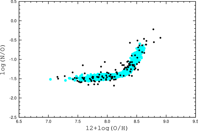
Figure 2: The O/H–N/O diagram. The filled gray (light-blue in the color version) circles show abundances derived using the NS-calibration for the sample of nearby SDSS galaxies. The filled black circles show $T_{e}$-based abundances in our sample of calibration H ii regions. (A color version of this figure is available in the online version.)

To verify the reliability of the NS-calibration, we compare the N/O–O/H diagram using the NS-calibration for SDSS spectra of H ii regions with that obtained from H ii regions in nearby galaxies with $T_{e}$-based abundances (the sample of calibration H ii regions). Line flux measurements in SDSS spectra have been carried out by several groups. Here, we use the data catalogs made publicly available by the MPA/JHU group . The techniques used to construct the catalogues are described in Brinchmann et al. (2004); Tremonti et al. (2004) and other publications by the same authors. We have chosen to use these catalogues instead of the original SDSS spectral database because the line flux measurements are generally more accurate.

We extracted emission-line objects from the MPA/JHU catalogs which satisfy the following criteria: (1) the redshift z$\la$0.023, (2) the equivalent widths of H$\alpha$, H$\beta$, [O iii]$\lambda$4959, [O iii]$\lambda$5007, [N ii]$\lambda$6584, [S ii]$\lambda$6717 and [S ii]$\lambda$6731 lines are larger than 3Å, 3) the line ratio 3.3$\ga$[O iii]$\lambda$5007/[O iii]$\lambda$4959$\ga$2.7. Since our calibrations are valid only in the low-density regime, we have just included objects with a reasonable value of the [S ii] line ratio, i.e., those with 1.1 $<$ F${}_{\rm[S\,II]\lambda 6717}$/F${}_{\rm[S\,II]\lambda 6731}$ $<$ 1.6. Applying these criteria, we selected 4339 spectra from the MPA/JHU catalogs. Measurements of the [N ii]$\lambda$6584 line are more reliable than those of the [N ii]$\lambda$6548 line. Hence, we have used N₂ = 1.33[N ii]$\lambda$6584 instead of the standard N₂ = [N ii]$\lambda$6548 + [N ii]$\lambda$6584. The emission fluxes are then corrected for interstellar reddening using the theoretical H$\alpha$/H$\beta$-ratio and the analytical approximation to the Whitford interstellar reddening law from Izotov et al. (1994). Occationally, the derived values of the extinction c(H$\beta$) are negative (but close to zero). In those cases we set c(H$\beta$)$=0$.

We have derived (O/H)_NS and (N/H)_NS for all H ii regions in the extracted SDSS sample. Fig. 2 shows the resultant O/H–N/O diagram. SDSS H ii regions are plotted with filled gray (light-blue in the color version) circles. For comparison, H ii regions in nearby galaxies with $T_{\rm e}$-based abundances (the sample of calibration H ii regions) are shown as filled black circles. Fig. 2 also shows that the SDSS H ii regions nicely follow the general trend in the N/O–O/H diagram traced by the H ii regions with $T_{\rm e}$-based abundances.

Figure 3: Radial distribution of oxygen abundances in the disk of the spiral galaxy M 101 determined in different ways. Upper panel: Distribution of (O/H)${}_{T_{e}}$ abundances for the $M$ sample (see text). The solid line is the best fit to the data. Middle panel: Distribution of (O/H)_NS abundances for the $M$ sample. The dashed line is the best fit to these data, the solid line is the same as in the upper panel. Lower panel: Distribution of (O/H)_NS abundances based on SDSS spectra. The dashed line is the best fit to these data, the solid line is the same as in the upper panel.

Figure 4: The same as in Fig. 3 but for nitrogen.

We have also tested the reliability of the NS-calibration using data for the spiral galaxy M 101 (=NGC 5457) as a reference. The radial distributions of oxygen and nitrogen abundances in the disk of M 101 are well established by the $T_{e}$-method, and the oxygen abundances in H ii regions in M 101 span a large interval of metallicity (about an order of magnitude), which provides a possibility to test the NS-calibration in different metallicity regimes. Furthermore, there are spectra for several dozens of H ii regions in M 101 in the SDSS spectral database.

The spectra of H ii regions in the disk of M 101 with measured electron temperatures $t_{3}$=$t$(O iii) or/and $t_{2}$=$t$(N ii) have been taken from Sedwick & Aller (1981); Rayo et al. (1982); McCall et al. (1985); Torres-Peimbert et al. (1989); Garnett & Kennicutt (1994); Kinkel & Rosa (1994); van Zee et al. (1998); Luridiana et al. (2002); Kennicutt et al. (2003); Izotov et al. (2007); Esteban et al. (2009). For the sake of brevity, this compilation of spectra will be referred to as the $M$ sample. The $M$ sample contains 47 measurements of electron temperature. It should be noted that a significant fraction (30 out of 47) of the $M$ sample is part of the sample of the calibration data points. The deprojected galactocentric distances of H ii regions normalised to the disk isophotal radius are taken from Kennicutt & Garnett (1996); Kennicutt et al. (2003).

Fig. 3 shows the radial distributions of oxygen abundances in the disk of M 101 determined in different ways. The upper panel shows the distribution of (O/H)${}_{T_{e}}$ abundances for the $M$ sample. The solid line is the linear least-square best fit to the data. The middle panel in Fig. 3 shows the radial distribution of (O/H)_NS abundances for the same $M$ sample. The dashed line shows a linear least-square fit to these data. The solid line is the same as in the upper panel. One can see that the scatter of (O/H)_NS abundances in the middle panel is lower respect to the scatter of (O/H)${}_{T_{e}}$ abundances in the upper panel. This may be evidence for that the larger scatter in the (O/H)${}_{T_{e}}$ abundances is caused, at least partly, by the uncertainties in the measurements of weak auroral lines.

The lower panel of Fig. 3 shows the radial distribution of (O/H)_NS abundances for the sample of selected SDSS spectra of H ii regions in the disk of the M 101 (line flux measurements in SDSS spectra have been taken from the MPA/JHU catalog using the selection criteria mentioned above). After correction for interstellar reddening, the oxygen (O/H)_NS and nitrogen (N/H)_NS abundances were determined using Eqs.(19),(31). The galactocentric distances of the SDSS H ii regions have been computed using the SDSS coordinates with a major axis position angle of 37°and an inclination between the line of sight and polar axis of 18°(Kennicutt & Garnett, 1996). The fractional distances R_G/R₂₅ have deen obtained with the isophotal radius R₂₅ = 14.4 arcmin taken from the Third Reference Catalog of bright Galaxies (de Vaucouleurs et al., 1991). The dashed line shows a linear least-square fit to these data. The solid line is the same as in the upper panel.

Fig. 3 shows that the oxygen abundances derived using the NS calibration for both the compilation of spectra and the SDSS spectra follow the radial gradient traced by the H ii regions with oxygen abundances determined with the direct method.

Fig. 4 shows the radial distributions of nitrogen abundances in the disk of M 101 determined in different ways. Again the upper panel shows the distribution of (N/H)${}_{T_{e}}$ abundances for the $M$ sample, the middle panel shows the radial distribution of (N/H)_NS abundances for the $M$ sample, and the lower panel shows the radial distribution of (N/H)_NS abundances for a sample of SDSS spectra of H ii regions in the disk of M 101. Again, the nitrogen abundances derived using the NS-calibration for both our compilation of spectra and the SDSS spectra, follow the radial gradient traced by the H ii regions with nitrogen abundances determined with the direct method.

The comparison between the scatter of the residuals for the NS-calibrations derived here, with the scatter of the residuals for the ONS-calibrations from Pilyugin et al. (2010), shows that the scatters are comparable in the case of O/H abundances and $t$ values, but in the case of N/H abundances the scatter of the residual for the NS-calibrations is significantly larger than that for the ONS-calibrations.

4 Conclusions

The [O ii]$\lambda$3727+$\lambda$3729 emission line is outside the wavelength range covered by SDSS spectra of nearby galaxies with redshift $z\la 0.023$. Hence, one needs a calibration for deriving abundances in H ii regions such that the calibration relations do not involve the nebular oxygen line [O ii]$\lambda$3727+$\lambda$3729. Such relations have been derived here using the spectra of H ii regions with measured electron temperatures as calibration datapoints.

The reliability of the NS-calibration has been verified by comparison between a N/O–O/H diagram computed via the NS-calibration for H ii regions from SDSS spectra and that for H ii regions having abundances determined through the direct method. We found that the NS-calibration-based abundances follow the general trend in the N/O–O/H diagram traced by the H ii regions with the $T_{e}$-based abundances.

Furthermore, the NS-calibration has also been tested by comparison between radial distributions of oxygen and nitrogen in the disk of the well-studied spiral galaxy M 101 determined in different ways. We found that the radial distributions of the NS-calibration-based oxygen and nitrogen abundances agree very well with the radial oxygen and nitrogen gradient traced by the H ii regions with abundances determined with the direct method.

We conclude that the NS-calibration provides reliable oxygen and nitrogen abundances over the whole range of metallicities typically found in H ii regions.

Though our study was motivated by the SDSS data for nearby H ii regions these calibrations can be applied to any spectra without a reliable measurement of the nebular oxygen line [O ii]$\lambda$3727+$\lambda$3729, i.e., the spectra of many low surface brightness galaxies. Moreover, calibrations can be used for the abundance determination in any H ii region independently whether the nebular oxygen line [O ii]$\lambda$3727+$\lambda$3729 is available or not.

References

- Alloin et al. (1979) Alloin D., Collin-Souffrin S., Joly M., & Vigroux L. 1979, A&A, 78, 200
- Brinchmann et al. (2004) Brinchmann J., Charlot S., White S.D.M., Tremonti C., Kauffmann G., Heckman T., & Brinkmann J. 2004, MNRAS, 351, 1151
- de Vaucouleurs et al. (1991) de Vaucouleurs G., de Vaucouleurs A., Corvin H.G., Buta R.J., Paturel J., & Fouque P. 1991, Third Reference Catalog of bright Galaxies (New York: Springer)
- Dopita & Evans (1986) Dopita M.A., & Evans I.N. 1986, ApJ, 307, 431
- Esteban et al. (2009) Esteban C., Bresolin F., Peimbert M., Carcía-Rojas J., Peimbert A., & Mesa-Delgado A. 2009, ApJ, 700, 654
- Garnett & Kennicutt (1994) Garnett D.R., & Kennicutt R.C. 1994, ApJ, 426, 123
- Izotov et al. (1994) Izotov Y.I., Thuan T.X., & Lipovetsky V.A., 1994, ApJ, 435, 647
- Izotov et al. (2007) Izotov Y.I., Thuan T.X. & Stasińska G. 2007, ApJ, 662, 15
- Kewley & Ellison (2008) Kewley L.J., & Ellison S.L. 2008, ApJ, 681, 1183
- Kennicutt et al. (2003) Kennicutt R.C., Bresolin F., & Garnett D.R. 2003, ApJ, 591, 801
- Kennicutt & Garnett (1996) Kennicutt R.C., & Garnett D.R. 1996, ApJ, 456, 504
- Kinkel & Rosa (1994) Kinkel U, & Rosa M.R. 1994, A&A, 228, L37
- Kniazev et al. (2004) Kniazev A.Y., Pustilnik S.A., Grebel E.K., Lee H., & Pramskij A.G. 2004, ApJSS, 153, 429
- Liang et al. (2006) Liang Y.C., Yin S.Y., Hammer F., Deng L.C., Flores H., & Zhang B. 2006, ApJ, 652, 257
- López-Sánchez & Esteban (2010) López-Sánchez Á.R., Esteban C. 2010, A&A, 517, id. A85
- Luridiana et al. (2002) Luridiana V., Esteban C., Peimbert M., & Peimbert A. 2002, Rev.Mex.A.A., 38, 97
- Magrini et al. (2007) Magrini L., Vílchez J.M., Mampaso A., Corradi R.L.M., & Leisy P. 2007, A&A, 470, 865
- McCall et al. (1985) McCall M.L., Rybski P.M., & Shields G.A. 1985, ApJS, 57, 1
- Pagel et al. (1979) Pagel B.E.J., Edmunds M.G., Blackwell D.E., Chun M.S., & Smith G. 1979, MNRAS, 189, 95
- Pérez-Montero & Contini (2009) Pérez-Montero E., & Contini T. 2009, MNRAS, 398, 949
- Pettini & Pagel (2004) Pettini M., & Pagel B.E.J. 2004, MNRAS, 348, 59L
- Pilyugin (2000) Pilyugin L.S. 2000, A&A, 362, 325
- Pilyugin (2001) Pilyugin L.S. 2001, A&A, 369, 594
- Pilyugin et al. (2009) Pilyugin L.S., Mattsson L., Vílchez J.M., & Cedrés B. 2009, MNRAS, 398, 485
- Pilyugin & Thuan (2005) Pilyugin L.S., & Thuan T.X. 2005, ApJ, 631, 231
- Pilyugin & Thuan (2007) Pilyugin L.S., & Thuan T.X. 2007, ApJ, 669, 2007
- Pilyugin et al. (2006) Pilyugin L.S., Thuan T.X., & Vílchez J.M. 2006, MNRAS, 367, 1139
- Pilyugin et al. (2010) Pilyugin L.S., Vílchez J.M., & Thuan T.X. 2010, ApJ, 720, 1738
- Rayo et al. (1982) Rayo J.F., Peimbert M., & Torres-Peimbert S. 1982, ApJ, 255, 1
- Sedwick & Aller (1981) Sedwick K.E., & Aller L.H., 1981, Proc. Nat. Acad. Sci. USA, 78, 1994
- Stasińska (2006) Stasińska G. 2006, A&A, 454, L127
- Thuan et al. (2010) Thuan T.X., Pilyugin L.S., & Zinchenko I.A. 2010, ApJ, 712, 1029
- Torres-Peimbert et al. (1989) Torres-Peimbert S., Peimbert M., & Fierro J. 1989, ApJ, 345, 186
- Tremonti et al. (2004) Tremonti C.A., Heckman T.M., Kauffmann G., & et al. 2004, ApJ, 613, 898
- van Zee et al. (1998) van Zee L., Salzer J.J., Haynes M.P., O‘Donoghiu A.A., & Balonek T.J. 1998, AJ, 116, 2805
- Vílchez & Esteban (1996) Vílchez J.M., & Esteban C. 1996, MNRAS, 280, 720
- York et al. (2000) York D.G., Anderson J.E., Anderson S.F., et al. 2000, AJ, 120, 1579