Renormalization of heavy-light currents in moving NRQCD

Abstract

Heavy-light decays such as $B\rightarrow\pi\ell\nu$, $B\rightarrow K^{*}\gamma$ and $B\rightarrow K^{(*)}\ell\ell$ can be used to constrain the parameters of the Standard Model and in indirect searches for new physics. While the precision of experimental results has improved over the last years this has still to be matched by equally precise theoretical predictions. The calculation of heavy-light form factors is currently carried out in lattice QCD. Due to its small Compton wavelength we discretize the heavy quark in an effective non-relativistic theory. By formulating the theory in a moving frame of reference discretization errors in the final state are reduced at large recoil. Over the last years the formalism has been improved and tested extensively. Systematic uncertainties are reduced by renormalizing the m(oving)NRQCD action and heavy-light decay operators. The theory differs from QCD only for large loop momenta at the order of the lattice cutoff and the calculation can be carried out in perturbation theory as an expansion in the strong coupling constant. In this paper we calculate the one loop corrections to the heavy-light vector and tensor operator. Due to the complexity of the action the generation of lattice Feynman rules is automated and loop integrals are solved by the adaptive Monte Carlo integrator vegas. We discuss the infrared and ultraviolet divergences in the loop integrals both in the continuum and on the lattice. The light quarks are discretized in the ASQTad and highly improved staggered quark (HISQ) action; the formalism is easily extended to other quark actions.

I Introduction

Decays of mesons containing heavy quarks provide an excellent laboratory for studying the heavy flavor sector of the Standard Model. For inclusive decays techniques such as quark-hadron duality and the operator product expansion have been used to predict decay amplitudes and spectra to high precision (see, for example Refs. Misiak et al. (2007); Gardi (2007)). Exclusive decays have a well defined hadronic final state and are easier to measure but obtaining precise theoretical predictions for these processes is more challenging since the quarks in the final state are bound inside a hadron. Nevertheless improving on these predictions is crucial to check results from inclusive measurements and overconstrain the parameters of the Standard Model to uncover the effects of putative new physics.

The decay $B\rightarrow\pi\ell\nu$ can, for instance, be used to constrain the magnitude of $V_{ub}$, one of the least known Cabibbo–Kobayashi–Maskawa (CKM) mixing matrix elements. In addition, rare decays like $B\rightarrow K^{*}\gamma$ or $B\rightarrow K^{(*)}\ell\ell$ are loop-suppressed in the Standard Model and expected to be sensitive to the presence of new physics Aliev et al. (2000a, b); Neubert (2002).

Precise calculations of hadronic matrix elements are needed to match experimental precision (which is still to improve further with new results from LHCb and the planned SuperB factory). Lattice QCD provides a model-independent framework for these calculations. It is, however, difficult to discretize the heavy valence quarks directly on lattices that are currently available since their Compton wavelength is comparable to the lattice spacing, $a$. To overcome this problem we use the effective lattice field theory NRQCD Lepage and Thacker (1988); Thacker and Lepage (1991); Davies and Thacker (1992); Lepage et al. (1992), which describes QCD in the non-relativistic limit where the heavy-quark velocity is much less than unity. NRQCD is useful for studying mesons with heavy-quark constituents such as $J/\psi$, $\Upsilon$, $D$ and $B$. The heavy-light vector form factor has been calculated in lattice NRQCD and combined with experimental data to extract $|V_{ub}|$ Dalgic et al. (2006). The hadronic form factors are functions of the squared momentum transfer $q^{2}=(p_{B}-p_{F})^{2}$, where $p_{B}$ and $p_{F}$ are the momenta of the decaying $B$ meson and the hadronic final state. Current lattice calculations using NRQCD work well only for large $q^{2}$, partially owing to large discretization errors in the hadronic final state. The radiative decay $B\rightarrow K^{*}\gamma$ has $q^{2}=0$, however, and most experimental data for $B\rightarrow\pi\ell\nu$ comes from the small $q^{2}$ region. The large extrapolation to small $q^{2}$ is a sizable source of systematic error in analyzing such decays and it is thus desirable to extend the range of accessible $q^{2}$ in a lattice calculation. In our approach, this is achieved by formulating the theory in a moving reference frame Sloan (1998). The frame velocity is chosen to reduce the three-momentum of the final hadron state at small $q^{2}$, and hence also suppress the associated lattice artifacts. This approach is known as moving NRQCD (mNRQCD) Foley and Lepage (2003); Foley (2004); Foley et al. (2005); Horgan et al. (2009). The momentum of the heavy quark $p=mu+p_{\mathrm{res}}$ is split into a contribution $mu$ associated with the frame velocity $u=(\gamma,\gamma\boldsymbol{v})$ and a residual momentum $p_{\mathrm{res}}$, which is of the order of the hadronic scale $\Lambda_{\mathrm{QCD}}$. The first contribution is treated exactly so that corrections can be expanded in powers of $p_{\mathrm{res}}/m$. Discretization errors, which scale with some power of $ap_{\mathrm{res}}$, can be removed systematically by improving the action.

Although we focus here on mNRQCD, we note that similar calculations are possible using other descriptions of moving heavy quarks Mandula and Ogilvie (1992); Hashimoto and Matsufuru (1996); Boyle (2004). A comparison of predictions from these different approaches would provide a valuable test of our understanding of the systematic errors in all these methods.

Hadronic matrix elements of heavy-light currents have been calculated using lattice mNRQCD by the HPQCD Collaboration Meinel et al. (2008); Liu et al. (2009). The NRQCD effective theory is obtained from QCD by integrating out the effects of physics on energy scales of order $m$ or larger; on the lattice this upper energy scale is determined by the lattice spacing, $a$. Operators in QCD are written as a formal expansion of operators defined in terms of the effective non-relativistic fields of NRQCD. The coefficients of the NRQCD operators in the expansion are determined as power series in the strong coupling constant $\alpha_{s}(q^{*}/a)$ which is defined in an appropriate renormalization scheme and where $q^{*}$ is a dimension parameter of order unity. The NRQCD operators are ordered in powers of $1/m$. For quarkonium matrix elements this gives a series in $\alpha_{s}$ and the quark relative velocity $v_{\operatorname{rel}}^{2}$ whereas for heavy-light systems the series is an expansion in $\alpha_{s}$ and $\Lambda_{\mathrm{QCD}}/m$. These coefficients are the radiative corrections which compensate for the missing contribution of ultraviolet modes in QCD which are omitted by the imposition of the high-momentum ultraviolet cutoff in the lattice formulation. QCD and the effective lattice theory agree for infrared scales sufficiently below the heavy quark mass $m$ and so the radiative corrections are governed by momenta larger than $m\gtrsim 1/a$ where the strong coupling constant is small. It is therefore legitimate to calculate these corrections in perturbation theory. The coefficients are computed by equating the matrix elements of the operator in QCD and of its NRQCD expansion for any choice of external states. Because the coefficients are independent of the matrix element chosen, we carry out the radiative matching calculation for appropriately chosen external on-shell quark states; this is the usual technique employed in matching calculations for NRQCD (see, for example, Morningstar and Shigemitsu (1998); Hart et al. (2007)). These radiative corrections are expected to be comparable in size to higher order corrections in the $1/m$ expansion.

Owing to the complexity of the lattice actions used, the generation of Feynman rules has been automated Lüscher and Weisz (1986); Hart et al. (2005, 2009) and the resulting integrals are calculated using the adaptive Monte Carlo integrator vegas Lepage (1978, 1980), possibly after smoothing the integrand by adding an infrared subtraction function. In Horgan et al. (2009) radiative corrections to the heavy quark action have been calculated for a range of frame velocities. In this work we extend this calculation to the matching coefficients for the leading order operators of the vector and tensor currents.

The outline of this paper is as follows. We discuss the different heavy-light continuum operators that contribute to $B\rightarrow\pi\ell\nu$ and rare $B$ decays in Sec. II, and we introduce the various quark actions used in this project in Sec. III. The central part of this work, the matching calculation between continuum and lattice operators, is presented in Sec. IV where we calculate one-loop matrix elements both in the continuum and in the effective lattice theory and combine them to obtain the matching coefficients. In Sec. V we present numerical results. We summarize and discuss our findings in Sec. VI.

Some preliminary results from this work appeared in Ref. Meinel et al. (2008); Muller et al. (2009); Liu et al. (2009).

II Continuum operators

In general we shall denote current operators by $J_{n}^{(\Gamma)}$ with the appropriate number of Lorentz indices and where $\Gamma$ labels the symmetry and transformation properties and the integer subscript, $n$, distinguishes different operators with the properties.

An example is the semileptonic decay $B\rightarrow\pi\ell\nu$ which occurs at tree level in the quark picture. It is mediated by the hadronic vector current

$$J_{0}^{(V)\mu}=\overline{q}_{L}\hat{\gamma}^{\mu}\Psi_{L},$$ (1)

where $q$ and $\Psi$ are the light- and heavy-quark spinors. We follow the convention in Appendix A of Ref. Horgan et al. (2009) for the Dirac gamma matrices $\hat{\gamma}^{\mu}$. Only left-handed particles (denoted by the subscript $L$) participate in the weak interaction. For massless leptons the total width of this decay is proportional to the square of the form factor $f_{+}(q^{2})$ defined by

$$\langle\pi(p^{\prime})|J_{0}^{(V)\mu}|B(p)\rangle = f_{+}(q^{2})\left(p^{\mu}+p^{\prime\mu}-\frac{M_{B}^{2}-M_{\pi}^{2}}{q^{2}}q^{\mu}\right)$$ (2)

$$+ f_{0}(q^{2})\frac{M_{B}^{2}-M_{\pi}^{2}}{q^{2}}q^{\mu}$$

and the CKM matrix element $V_{ub}$.

The situation is more complicated for rare $B$ decays which can only occur at loop level in the Standard Model. After integrating out physics at the electroweak scale, the transition is described by a set of effective operators $Q_{j}$ with their associated Wilson coefficients $C_{j}(\mu)$ Buras (1998). For the radiative decay $B\rightarrow K^{*}\gamma$ the Hamiltonian is

$$\mathcal{H}=-\frac{4G_{F}}{\sqrt{2}}V_{tb}V_{ts}^{*}\sum_{j}C_{j}(\mu)\;Q_{j}$$ (3)

where the operator basis $Q_{j}$ used in this work is given, for example, in Refs. Greub et al. (1996); Ghinculov et al. (2004):

$$Q_{1} = (\overline{c}_{L\beta}\hat{\gamma}^{\mu}b_{L\alpha})(\overline{s}_{L\alpha}\hat{\gamma}_{\mu}c_{L\beta}),$$ (4)

$$Q_{2} = (\overline{c}_{L\alpha}\hat{\gamma}^{\mu}b_{L\alpha})(\overline{s}_{L\beta}\hat{\gamma}_{\mu}c_{L\beta}),$$

$$Q_{3} = (\overline{s}_{L\alpha}\hat{\gamma}^{\mu}b_{L\alpha})\sum_{q=u,d,c,s,b}(\overline{q}_{L\beta}\hat{\gamma}_{\mu}q_{L\beta}),$$

$$Q_{4} = (\overline{s}_{L\alpha}\hat{\gamma}^{\mu}b_{L\beta})\sum_{q=u,d,c,s,b}(\overline{q}_{L\beta}\hat{\gamma}_{\mu}q_{L\alpha}),$$

$$Q_{5} = (\overline{s}_{L\alpha}\hat{\gamma}^{\mu}b_{L\alpha})\sum_{q=u,d,c,s,b}(\overline{q}_{R\beta}\hat{\gamma}_{\mu}q_{R\beta}),$$

$$Q_{6} = (\overline{s}_{L\alpha}\hat{\gamma}^{\mu}b_{L\beta})\sum_{q=u,d,c,s,b}(\overline{q}_{R\beta}\hat{\gamma}_{\mu}q_{R\alpha}),$$

$$Q_{7} = \frac{e}{16\pi^{2}}m_{b}\overline{s}_{L\alpha}\sigma^{\mu\nu}b_{R\alpha}F_{\mu\nu},$$

$$Q_{8} = \frac{g}{16\pi^{2}}m_{b}\overline{s}_{L\alpha}\sigma^{\mu\nu}T^{a}_{\alpha\beta}b_{R\beta}G_{\mu\nu}^{a},$$

with

$$\sigma^{\mu\nu}=\frac{i}{2}[\hat{\gamma}^{\mu},\hat{\gamma}^{\nu}].$$ (5)

$F_{\mu\nu}$ ($G^{a}_{\mu\nu}$) is the electromagnetic (chromodynamic) field strength tensor; $\alpha$ and $\beta$ are color indices.

This factorization separates the physics at large energy scales, which is contained in the model-dependent Wilson coefficients $C_{j}(\mu)$, from the universal hadronic matrix elements of the effective operators $Q_{j}$.

$C_{1}$	$0.016$	$C_{5}$	$0.017$
$C_{2}$	$0.711$	$C_{6}$	$0.009$
$C_{3}$	$-0.078$	$C_{7}$	$-0.300$
$C_{4}$	$0.093$	$C_{8}$	$-0.144$

Table 1: Numerical values of the Standard Model Wilson coefficients in the effective Lagrangian (3) for the radiative decay $B\rightarrow K^{*}\gamma$. The coefficients $C_{j}(\mu_{b})$ are evaluated in the leading logarithmic (LL) approximation at the scale $\mu_{b}=5.0\operatorname{MeV}$ using the so-called “magic numbers” in Ref. Buras (1998) with $m_{Z}=91.1876\operatorname{MeV}$, $m_{W}=\mu_{W}=80.425\operatorname{MeV}$ and $\alpha_{s}(m_{Z})=0.118$.

II.1 Wilson coefficients

By matching the effective Hamiltonian in Eqn. (3) to the Standard Model it is easy to see that at tree level $C_{2}=1$ and all other coefficients are zero. After summing the leading logarithms of the form $\left[\alpha_{s}\log(\mu_{W}/\mu_{b})\right]^{n}$ the dominant contribution to $C_{7}$ comes from the mixing of $Q_{2}$ to $Q_{7}$ via one loop diagrams Buras (1998). The Standard Model Wilson coefficients relevant for the radiative decay are given in Tab. 1 in the leading logarithmic (LL) approximation. As can be seen from these numbers, the dominant operators are $C_{2}$ and $C_{7}$. Numerical values of $C_{j}$ are now known at next-to-next-to-leading (NNLL) order in the Standard Model Misiak et al. (2007).

The Wilson coefficients are model dependent. For example, in Grinstein et al. (1990) it is shown how $C_{7}(\mu_{W})$ and $C_{8}(\mu_{W})$ change in a two Higgs doublet model. The numerical size of these changes depends on the parameters of the specific model. In Grinstein et al. (1990) it is reported that the inclusive decay rate $B\rightarrow X_{s}\gamma$, which in the LL approximation is proportional to $|C_{7}(\mu_{b})|^{2}$, could in principle be enhanced by about a factor of three compared to the Standard Model.

Although this enhancement is now ruled out by recent calculations of the Standard Model branching ratio in the inclusive $B\rightarrow X_{s}\gamma$ Misiak et al. (2007); Becher and Neubert (2007) and exclusive $B\rightarrow K^{*}\gamma$ Ali et al. (2008); Ball et al. (2007); Becher et al. (2005) decays, which are compatible with experimental results Barberio et al. (2008), the situation is less clear for the time dependent CP asymmetry in the exclusive decay: although it is expected to be small in the Standard Model Ball and Zwicky (2006) it has not yet been measured to sufficiently high precision Aubert et al. (2005); Ushiroda et al. (2006). In the Standard Model the opposite chirality operator, which is obtained by replacing $b_{R}\mapsto b_{L}$ and $s_{L}\mapsto s_{R}$ in $Q_{7}$ is suppressed by a factor of $m_{s}/m_{b}$ as the spin flip requires the insertion of a mass term. This is not necessarily the case in the new physics models studied in Atwood et al. (1997) where it is shown that the opposite chirality operator and mixing induced CP asymmetries can be enhanced even if the branching ratio agrees with Standard Model predictions.

Similar conclusions can be drawn for the decay $B\rightarrow K^{(*)}\ell\ell$ Ali et al. (2000, 2002), the forward-backward asymmetry is dependent on $C_{7}$, $C_{9}$ and $C_{10}$. The current experimental measurements Aubert et al. (2006); Adachi et al. (2008); Aaltonen et al. (2009) will be improved by the LHCb experiment Schune (2009) and help constrain these coefficients.

II.2 Local and non-local operators

The operators in Eqns. (3,4) can be split into two groups: the four quark operators 1-6 couple two hadronic currents at one point in space time. All other operators couple a heavy-light quark current to a gauge boson or a leptonic current. These two sets of operators contribute differently to hadronic heavy-light matrix elements Grinstein and Pirjol (2000).

II.2.1 Local contributions

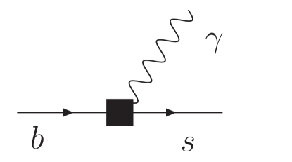
Figure 1: Local tensor operator diagram contributing to the decay $B\rightarrow K^{*}\gamma$

The local contribution to the radiative decay $B\rightarrow K^{*}\gamma$ is described by the tensor current (see Fig. 1)

$$Q_{7}=\frac{e}{16\pi^{2}}m(\overline{q}_{L}\sigma^{\mu\nu}\Psi_{R})F_{\mu\nu}.$$ (6)

The local contributions to the leptonic decay $B\rightarrow K^{(*)}\ell\ell$ also include operators

$$Q_{9} =\frac{e^{2}}{16\pi^{2}}\overline{q}_{L}\hat{\gamma}^{\mu}\Psi_{L}\sum_{\ell}\overline{\ell}\hat{\gamma}_{\mu}\ell,$$

$$Q_{10} =\frac{e^{2}}{16\pi^{2}}\overline{q}_{L}\hat{\gamma}^{\mu}\Psi_{L}\sum_{\ell}\overline{\ell}\hat{\gamma}_{\mu}\hat{\gamma}^{5}\ell,$$ (7)

which couple the heavy-light vector current $J_{0}^{(V)\mu}$ to a vector (or axial vector) leptonic current.

In the following we will consider the vector current in Eqn. (1) and the heavy-light hadronic tensor current

$$J_{0}^{(T)\mu\nu}=m(\overline{q}_{L}\sigma^{\mu\nu}\Psi_{R}).$$ (8)

The heavy quark mass is included in this current as only left-handed particles participate in the weak interaction: flipping the chirality on one of the external legs requires the insertion of a mass term $m\overline{q}_{L}q_{R}+(\mathrm{h.c.})$. Whilst in the Standard Model the operator $m_{q}(\overline{q}_{R}\sigma^{\mu\nu}\Psi_{L})$ with opposite chirality is suppressed by $m_{q}/m$ relative to Eqn. (8), this is not necessarily the case in new physics models Atwood et al. (1997).

As we set the light quark mass to zero in the matching calculation we will drop all chiral projectors in the following.

II.2.2 Non-local contributions

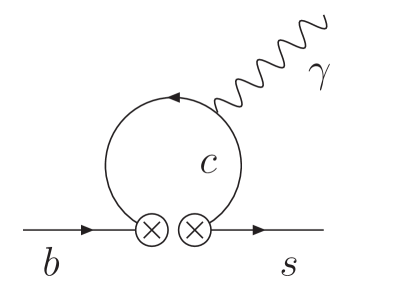
Figure 2: Non-local four quark operator diagram contributing to the decay $B\rightarrow K^{*}\gamma$

Non-local contributions come from diagrams like the one in Fig. 2: The gauge bosons couple to an internal quark loop which is created by contracting the two charm fields of a four quark operator. Given the size of $C_{2}$ it is important to estimate the effect of these diagrams on the hadronic matrix element.

Long distance effects.

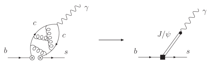
Figure 3: Resonant contribution to $b\rightarrow s\gamma$ from four quark operators.

The dominant contribution to the long distance amplitude induced by the $b\rightarrow s\overline{c}c$ operators is usually assumed to come from the diagram where the photon couples directly to the charm quark loop. This is confirmed by the perturbative calculation combined with a quark model in Asatrian et al. (1999) where it is found that the main contribution generated by $Q_{2}$ is given by diagrams where the photon couples to the $\overline{c}c$ loop and the gluon connects this loop to either the $b$ or $s$ quark. Only $Q_{7}$ contributes at tree level but in Asatrian et al. (1999) it is argued that the $\mathcal{O}(\alpha_{s})$ contribution of the four quark operator is of the same order as the one loop correction to the electromagnetic tensor operator $Q_{7}$.

The resonant contribution from the charm loop can be described as the decay $B\rightarrow V\psi_{n}$, where the $\psi_{n}$ is a bound $\overline{c}c$ vector state, such as $J/\psi$, which subsequently decays into a photon, see Fig. 3.

In this approximation the long-distance amplitude can be written as

$$A =Q_{c}e\sum_{n,\epsilon_{n}}\frac{(\epsilon^{*}_{n})_{\mu}\langle 0|\overline{c}\hat{\gamma}^{\mu}c|\psi_{n}\rangle\mathcal{A}(B\rightarrow V\psi_{n})}{q^{2}-M_{n}^{2}+iM_{n}\Gamma_{n}}.$$ (9)

where $\epsilon_{n}$ is the polarization of the vector meson $\psi_{n}$ with mass $M_{n}$ and width $\Gamma_{n}$. For real photons with $q^{2}=0$ the sum is dominated by the lowest lying resonances. The mass of the $J/\psi$ is $3.097\operatorname{GeV}$ so that long distance effects from charm loops are expected to be suppressed by the inverse of this mass.

This argument is supported by the explicit calculation in Khodjamirian et al. (1997) where the charm quark is integrated out to obtain an effective $b\overline{s}g\gamma$ operator suppressed by $1/m_{c}^{2}$. The matrix element of this local operator is calculated using QCD sum rules and found to be small, contributing around $5\%$ of the dominant amplitude from $Q_{7}$.

Chromomagnetic tensor operator.

The contribution from the chromomagnetic tensor operator is estimated in Carlson and Milana (1995). There the decay amplitude is calculated for both the electromagnetic and the tensor operator in the framework of a quark model. The contribution of $Q_{8}$ is found to be suppressed relative to $Q_{7}$ by a factor $\Lambda_{\operatorname{QCD}}/m_{B}\times C_{8}/C_{7}\approx 5\%$.

To summarize, matrix elements of four quark operators and of the chromomagnetic tensor operator are suppressed for small $q^{2}$ and it is likely that they contribute little to the radiative decay. With currently available techniques these non-local contributions can not be treated in lattice QCD and, if required, must be calculated using different approaches, such as QCD sum rules Cheng (1995); Greub et al. (1995); Carlson and Milana (1995); Khodjamirian et al. (1997); Asatrian et al. (1999); Ball and Zwicky (2005); Ball et al. (2007) to complement the lattice calculation of the local operators. In the following we will concentrate on the vector current $\overline{q}_{L}\hat{\gamma}^{\mu}\Psi_{L}$ and the tensor current $m(\overline{q}_{L}\sigma^{\mu\nu}\Psi_{R})$ which are the hadronic parts of the electroweak operators in (6) and (7). Nonperturbative lattice matrix elements elements of these currents have been calculated Meinel et al. (2008); Liu et al. (2009) by using mNRQCD as an effective theory for the heavy quark.

III Lattice quark actions

On currently available lattices the Compton wavelength of the $b$ quark is smaller than the lattice spacing. We discretize the heavy quark in an effective, non-relativistic theory where the high frequency fluctuations have been integrated out. The construction of this action is described in Horgan et al. (2009) and in the following we summarize the main results.

The light quarks are discretized using highly improved relativistic actions Lepage (1999); Follana et al. (2007). In the one loop calculations presented in this paper vacuum polarization effects of the light quark do not contribute.

III.1 Moving NRQCD

The (tree level) NRQCD action is obtained by decoupling the quark and antiquark degrees of freedom in the fermionic action by a Foldy-Wouthuysen-Tani transformation. The theory can be Lorentz-transformed to a moving frame and higher order time derivatives are removed by a subsequent field transformation. On the lattice, where Lorentz invariance is broken by discretization, this will give rise to a new theory which is known as m(oving) NRQCD. As the theory contains only first order time derivatives, propagators can be computed very efficiently by a single sweep through the lattice.

The mNRQCD action is given by

$$S=\sum_{\boldsymbol{x},\tau}\psi^{\dagger}(\boldsymbol{x},\tau)\left[\psi(\boldsymbol{x},\tau)-K(\tau)\psi(\boldsymbol{x},\tau-1)\right]$$ (10)

with kernel

$$K(\tau)=\left(1-\frac{\delta H}{2}\right)\left(1-\frac{H_{0}}{2n}\right)^{n}U_{4}^{\dagger}(\boldsymbol{x},\tau-1)\\ \times\left(1-\frac{H_{0}}{2n}\right)^{n}\left(1-\frac{\delta H}{2}\right).$$ (11)

The lowest order kinetic term $H_{0}$ is

$$H_{0}=-i\boldsymbol{v}\cdot\boldsymbol{\Delta}^{\pm}-\frac{\Delta^{(2)}-\Delta_{v}^{(2)}}{2\gamma m}$$ (12)

where $\boldsymbol{v}$ is the frame velocity and $\Delta_{j}^{\pm}$, $\Delta^{(2)}$ and $\Delta_{v}^{(2)}$ are first and second order gauge covariant finite difference operators defined in Ref. Horgan et al. (2009). In momentum space the non-relativistic dispersion relation

$$E =\boldsymbol{v}\cdot\boldsymbol{p}_{\mathrm{res}}+\frac{\boldsymbol{p}_{\mathrm{res}}^{2}-(\boldsymbol{v}\cdot\boldsymbol{p}_{\mathrm{res}})^{2}}{2\gamma m}+\dots$$

$$\approx\sqrt{m^{2}+(m\gamma\boldsymbol{v}+\boldsymbol{p}_{\mathrm{res}})^{2}}-\gamma m$$

$$=\sqrt{m^{2}+\boldsymbol{p}^{2}}-\gamma m$$ (13)

is obtained. $\delta H$ contains higher order corrections in $1/m$ and operators which remove discretization errors. The action used in this work is described in Ref. Horgan et al. (2009); it is correct to $\mathcal{O}(1/m^{2},v_{\operatorname{rel}}^{4})$, where $v_{\operatorname{rel}}$ is the relative velocity of the two quarks in a heavy-heavy system.

The integer stability parameter $n$ is introduced to remove numerical instabilities for smaller quark masses $m$.

III.2 Relativistic quark actions

We separately consider two different staggered lattice actions describing the light quarks.

The ASQTad action Lepage (1999) suppresses “taste-breaking” interactions of lattice doublers by $\mathcal{O}(\alpha_{s}a^{2})$. This is done by introducing form factors for one gluon emission in the action. The Highly Improved Staggered Quark (HISQ) action reduces discretization errors further by an additional level of smearing followed by link unitarization Follana et al. (2007).

Physically, the light quark mass is much smaller than the hadronic scale and in the matching calculation it will be set to zero. This simplifies the calculation and leads to additional relations between different matching coefficients due to chiral symmetry.

The MILC and UKQCD Collaborations have produced a set of lattice configuration ensembles including ASQTad vacuum polarization effects and are currently extending this to configurations with dynamical HISQ fermions Bazavov et al. (2008, 2009). These configurations are used in the nonperturbative calculation of heavy-light form factors Meinel et al. (2008); Liu et al. (2009).

IV Matching calculation

To match heavy-light operators, expressed in terms of effective mNRQCD heavy quark fields, to those in the continuum theory, we must calculate radiative corrections both in the continuum and on the lattice. We match the theories at leading order in the $1/m$ expansion and one loop order in $\alpha_{s}$. Matrix elements of $\mathcal{O}(1/m)$ operators are expected to be of the same size as the leading radiative corrections and are matched at tree level.

IV.1 Continuum calculation

In the continuum we calculate the one loop matrix elements of the currents $J_{0}^{(\Gamma)}$ and expand the result in inverse powers of the heavy quark mass. We use the notation $\Gamma=V,T$ to denote the expressions in Eqns. (1,8). Owing to Lorentz invariance these expansions can be expressed as linear combinations of a small number of tree level matrix elements:

$$\langle q|J_{0}^{(\Gamma)}|b\rangle_{\mathrm{con}}=\sum_{j}Z_{j}^{(\Gamma,\mathrm{con})}\langle q|J_{j}^{(\Gamma)}|b\rangle_{\mathrm{tree}}.$$ (14)

At leading order in the $1/m$ expansion the operators that contribute to the vector current are:

$$J_{0}^{(V)\mu} =\overline{q}\hat{\gamma}^{\mu}\Psi,$$

$$J_{1}^{(V)\mu} =\overline{q}u^{\mu}\Psi$$ (15)

and to the tensor current:

$$J_{0}^{(T)\mu\nu} =m(\overline{q}\sigma^{\mu\nu}\Psi),$$

$$J_{1}^{(T)\mu\nu} =2im\left(\overline{q}(\hat{\gamma}^{\mu}u^{\nu}-u^{\mu}\hat{\gamma}^{\nu})\right)\Psi$$ (16)

where $u^{\mu}=(\gamma,\gamma\boldsymbol{v})$ is the frame velocity. The one loop contributions to the mixing matrix $Z_{j}^{(\Gamma,\mathrm{con})}=\delta_{j0}+\alpha_{s}\delta Z_{j}^{(\Gamma,\mathrm{con})}+\dots$ are for the vector operator Morningstar and Shigemitsu (1998)

$$\delta Z_{0}^{(V,\mathrm{con})} =\frac{1}{3\pi}\left(-\frac{11}{4}-\frac{3}{2}\log\lambda^{2}/m^{2}\right),$$

$$\delta Z_{1}^{(V,\mathrm{con})} =\frac{2}{3\pi},$$ (17)

and for the tensor operator

$$\delta Z_{0}^{(T,\mathrm{con})} =\frac{1}{3\pi}\left(-\frac{27}{4}-\frac{3}{2}\log\lambda^{2}/m^{2}+4\log m^{2}/\mu^{2}\right),$$

$$\delta Z_{1}^{(T,\mathrm{con})} =0.$$ (18)

We introduced a gluon mass $\lambda$ to regulate infrared divergences. It is important to use the same infrared regulator in both continuum QCD and the effective lattice theory, any dependence on the gluon mass will cancel in the matching coefficients.

As the tensor current is not conserved, its anomalous dimension does not vanish:

$$\gamma_{T}^{(\mathrm{con})}=\frac{8\alpha_{s}}{3\pi}+\dots.$$ (19)

The coefficients of the infrared logarithms in Eqns. (17) and (18) agree due to heavy quark symmetry.

IV.2 Construction of lattice operators

On the lattice we must construct operators $J_{0}^{(\Gamma,\mathrm{lat})}$ which have the same on-shell matrix elements as the associated continuum operators:

$$\langle q|J_{0}^{(\Gamma,\mathrm{lat})}|b\rangle_{\mathrm{lat}}=\langle q|J_{0}^{(\Gamma)}|b\rangle_{\mathrm{con}}.$$ (20)

At tree level, the operators in the effective theory are obtained from Eqns. (1,8) by applying the field transformation

$$\Psi(x)=S(\Lambda)\tilde{T}(\tilde{x})e^{-im\hat{\gamma}^{0}u\cdot x}A_{D_{t}}\frac{1}{\sqrt{\gamma}}\Psi_{v}.$$ (21)

$S(\Lambda)$ is a spinorial Lorentz boost, $\tilde{T}$ the FWT transformation decoupling the quark- and antiquark fields in the rest frame and $A_{D_{t}}$ an additional field transformation to remove higher order time derivatives. $\Psi_{v}(x)=\left(\psi_{v}(x),0\right)^{T}$ is the (positive energy) field in the effective theory.

Using the explicit expressions in Ref. Horgan et al. (2009) one finds at $\mathcal{O}(1/m)$

$$\Psi=\frac{1}{\sqrt{\gamma}}\left(1-\frac{i\hat{\gamma}_{0}\boldsymbol{v}\cdot\boldsymbol{D}}{2m}+\frac{i\boldsymbol{\hat{\gamma}}\cdot\boldsymbol{D}}{2m}+\frac{i\boldsymbol{v}\cdot\boldsymbol{D}}{2\gamma m}\right)S(\Lambda)\Psi_{v}$$ (22)

from which the tree level currents in the effective theory can be read off by inserting the field transformation in Eqns. (1,8).

In the following we calculate the one loop matching coefficients of the leading order operators in the $1/m$ expansion. At this order both $\tilde{T}$ and $A_{D_{t}}$ are equal to the identity. The Lorentz boost is

$$S(\Lambda)=\frac{1}{\sqrt{2(1+\gamma)}}\left((1+\gamma)-\gamma v\hat{\boldsymbol{v}}\cdot\boldsymbol{\hat{\gamma}}\hat{\gamma}^{0}\right).$$ (23)

We choose $\hat{\boldsymbol{v}}$, the direction of the frame velocity, to be along one of the lattice axes, i.e. $\hat{\boldsymbol{v}}=(1,0,0)$. We can then classify the lattice directions (and associated Lorentz indices) as timelike (denoted 0, as usual), parallel to $\hat{\boldsymbol{v}}$ (denoted $\parallel$) or perpendicular to $\hat{\boldsymbol{v}}$ (denoted $\perp$).

IV.2.1 Choice of operator basis

In the continuum the operator basis $J_{0}^{(\Gamma)}$, $J_{1}^{(\Gamma)}$ is used. On the lattice Lorentz invariance is broken and it is convenient to work in another basis which is spanned by operators with different Dirac structure. Firstly, the operators $J_{0}^{(\Gamma)}$ and $J_{1}^{(\Gamma)}$ are split into the sum of two operators $J_{n}^{(\Gamma)}=J_{n,1}^{(\Gamma)}+J_{n,2}^{(\Gamma)}$. For $n=0$:

$$J_{0,1}^{(\Gamma)} =\rho^{(\Gamma)}f_{1}(v)\overline{q}(x)\Gamma\Psi_{v},$$

$$J_{0,2}^{(\Gamma)} =-\rho^{(\Gamma)}f_{2}(v)\overline{q}(x)\Gamma\boldsymbol{\hat{v}}\cdot\boldsymbol{\hat{\gamma}}\hat{\gamma}^{0}\Psi_{v}\;.$$ (24)

In the vector case $\Gamma=\hat{\gamma}^{\mu}$ and $\rho^{(V)}=1$, and in the tensor case $\Gamma=\sigma^{\mu\nu}$ and $\rho^{(T)}=m$. The velocity dependence has been absorbed in the functions

$$f_{1}(v) =\sqrt{\frac{1+\gamma}{2\gamma}}, f_{2}(v) =v\sqrt{\frac{\gamma}{2(1+\gamma)}}\;.$$ (25)

The corresponding leading order (in the heavy quark expansion) operators $J_{1,j}^{(\Gamma)}$ are obtained by replacing $\Gamma\mapsto u^{\mu}$ in the vector case, and $\Gamma\mapsto 2i(\hat{\gamma}^{\mu}u^{\nu}-\hat{\gamma}^{\nu}u^{\mu})$ for the tensor.

The tree level matrix elements of all these operators form a basis for expanding higher order matrix elements. In the following we do not, however, need to include $J_{1,j}^{(\Gamma)}$, because the tree level matrix elements are given by linear combinations of those of $J_{0,j}^{(\Gamma)}$ due to heavy quark symmetry $\hat{\gamma}^{0}\Psi_{v}=\Psi_{v}$. In the vector case:

$$J_{1,1}^{(V)0} =\gamma J_{0,1}^{(V)0}, J_{1,2}^{(V)0} =-\gamma J_{0,2}^{(V)0},$$

$$J_{1,1}^{(V)\parallel} =(1+\gamma)J_{0,2}^{(V)\parallel}, J_{1,2}^{(V)\parallel} =(1-\gamma)J_{0,1}^{(V)\parallel},$$ (26)

and for the tensor operator:

$$J_{1,1}^{(T)0\parallel} =2\left(\gamma J_{0,1}^{(T)0\parallel}+(1+\gamma)J_{0,2}^{(T)0\parallel}\right),$$

$$J_{1,2}^{(T)0\parallel} =2\left((1-\gamma)J_{0,1}^{(T)0\parallel}-\gamma J_{0,2}^{(T)0\parallel}\right),$$

$$J_{1,1}^{(T)0\perp} =2\gamma J_{0,1}^{(T)0\perp},$$

$$J_{1,2}^{(T)0\perp} =-2\gamma J_{0,2}^{(T)0\perp},$$

$$J_{1,1}^{(T)\parallel\perp} =-2(1+\gamma)J_{0,2}^{(T)\parallel\perp},$$

$$J_{1,2}^{(T)\parallel\perp} =-2(1-\gamma)J_{0,1}^{(T)\parallel\perp}.$$ (27)

Clearly, this decomposition is not Lorentz invariant, but can be carried out for fixed frame velocity.

On the lattice the two operators in Eqn. (24) mix under renormalization,

$$\langle q|J_{0,j}^{(\Gamma)}|b\rangle_{\mathrm{lat}}=\sum_{k}\left(\delta_{jk}+\alpha_{s}\delta Z^{(\Gamma,\mathrm{lat})}_{jk}+\dots\right)\times\\ \langle q|J_{0,k}^{(\Gamma)}|b\rangle_{\mathrm{tree}}\;,$$ (28)

(with $j,k=1,2$). Instead of using this basis (which we will call the $(1,2)$ basis), it is more convenient to work in the $(+,-)$ basis:

$$J_{0,\pm}^{(\Gamma)}=J_{0,1}^{(\Gamma)}\pm J_{0,2}^{(\Gamma)},$$ (29)

as only $J_{0,+}^{(\Gamma)}$ contributes to processes at tree level. We may then write

$$\langle q|J_{0,+}^{(\Gamma)}|b\rangle_{\mathrm{con}}=(1+\alpha_{s}\delta Z_{+}^{(\Gamma,\mathrm{con})})\langle q|J_{0,+}^{(\Gamma)}|b\rangle_{\mathrm{tree}}+\\ \alpha_{s}\delta Z_{-}^{(\Gamma,\mathrm{con})}\langle q|J_{0,-}^{(\Gamma)}|b\rangle_{\mathrm{tree}}.$$ (30)

On the lattice renormalization factors $\delta Z_{jk}^{(\Gamma,\mathrm{lat})}$ in this basis can then be defined in an analogous way to Eqn. (28) [i.e. where $j,k=\pm$]. For the vector operator, we must distinguish whether the Lorentz index of the current is timelike, parallel or perpendicular to the frame velocity. Relations like Eqn. (26) can then be used to relate $Z_{\pm}^{(V,\mathrm{con})}$ to $Z_{0}^{(V,\mathrm{con})}$ and $Z_{1}^{(V,\mathrm{con})}$:

$$\delta Z_{+}^{(V,\mathrm{con})0} =\delta Z_{0}^{(V,\mathrm{con})},$$

$$\delta Z_{-}^{(V,\mathrm{con})0} =\gamma\delta Z_{1}^{(V,\mathrm{con})},$$

$$\delta Z_{+}^{(V,\mathrm{con})\parallel} =\delta Z_{0}^{(V,\mathrm{con})}+\delta Z_{1}^{(V,\mathrm{con})},$$

$$\delta Z_{-}^{(V,\mathrm{con})\parallel} =-\gamma\delta Z_{1}^{(V,\mathrm{con})},$$

$$\delta Z_{+}^{(V,\mathrm{con})\perp} =\delta Z_{0}^{(V,\mathrm{con})},$$

$$\delta Z_{-}^{(V,\mathrm{con})\perp} =0\;.$$ (31)

For the tensor operator there is no dependence on the Lorentz indices:

$$\delta Z_{+}^{(T,\mathrm{con})} =\delta Z_{0}^{(T,\mathrm{con})},$$

$$\delta Z_{-}^{(T,\mathrm{con})} =0\;.$$ (32)

IV.2.2 Matching coefficients

Combining Eqns. (28,30), the lattice operator which has the same one loop matrix elements as the continuum operator is

$$J_{0}^{(\Gamma,\mathrm{lat})}=\left(1+\alpha_{s}c_{+}^{(\Gamma)}\right)J_{0,+}^{(\Gamma)}+\alpha_{s}c_{-}^{(\Gamma)}J_{0,-}^{(\Gamma)}$$ (33)

with

$$c_{+}^{(\Gamma)} =\delta Z_{+}^{(\Gamma,\mathrm{con})}-\delta Z_{++}^{(\Gamma,\mathrm{lat})},$$

$$c_{-}^{(\Gamma)} =\delta Z_{-}^{(\Gamma,\mathrm{con})}-\delta Z_{+-}^{(\Gamma,\mathrm{lat})}\;.$$ (34)

IV.3 Mixing matrix

In the $(1,2)$ basis of operators, the lattice mixing matrix can be split into a diagonal part and a contribution $\xi_{jk}^{(\Gamma)}$ from one particle irreducible (1PI) diagrams,

$$\delta Z_{jk}^{(\Gamma,\mathrm{lat})}=\left(\delta Z_{\mathrm{mult}}^{(\Gamma)}-\delta Z_{f_{j}}\right)\delta_{jk}+\xi_{jk}^{(\Gamma)}.$$ (35)

For the vector current the multiplicative renormalization contains the wavefunction renormalization only: $\delta Z_{\mathrm{mult}}^{(V)}=\frac{1}{2}\left(\delta Z_{q}+\delta Z_{\psi}\right)$. For the tensor current, however, there is an additional contribution from the renormalization of the heavy quark mass: $\delta Z_{\mathrm{mult}}^{(T)}=\frac{1}{2}\left(\delta Z_{q}+\delta Z_{\psi}\right)-\delta Z_{m}$.

The relation between renormalized and bare parameters is $\boldsymbol{v}_{R}=Z_{v}v$, $\gamma_{R}=(1-\boldsymbol{v}_{R}^{2})^{-1/2}$, $m_{R}=Z_{m}m$ and $q=\sqrt{Z_{q}}q_{R}$, $\Psi=\sqrt{Z_{\psi}}\Psi_{R}$. $m_{R}$ is the pole mass, which can be defined perturbatively both in the continuum and on the lattice. The renormalization constants can be expanded perturbatively using the generic formula $Z_{x}=1+\alpha_{s}\delta Z_{x}+\dots$.

The renormalization of the velocity functions $f_{1,2}$ in Eqn. (25) is $f_{j,R}=Z_{f_{j}}f_{j}$ with

$$\delta Z_{f_{1}} =\frac{1-\gamma}{2}\delta Z_{v}, \delta Z_{f_{2}} =\frac{1+\gamma}{2}\delta Z_{v}.$$ (36)

One then finds

$$\delta Z_{++}^{(\Gamma,\mathrm{lat})} =\delta Z_{\mathrm{mult}}^{(\Gamma)}-\frac{1}{2}\delta Z_{v}+\xi_{++}^{(\Gamma)},$$

$$\delta Z_{+-}^{(\Gamma,\mathrm{lat})} =\frac{\gamma}{2}\delta Z_{v}+\xi_{+-}^{(\Gamma)}.$$ (37)

Even though we use only the leading order heavy-light operators we still include $1/m$ corrections in the action. Next we isolate infrared divergences in the renormalization constants and find (in Feynman gauge)

$$\delta Z_{q} =\frac{1}{3\pi}\log a^{2}\lambda^{2}+F_{q},$$

$$\delta Z_{\psi} =-\frac{2}{3\pi}\log a^{2}\lambda^{2}+F_{\psi}(v,am),$$

$$\delta Z_{m} =F_{m}(v,am),$$

$$\delta Z_{v} =F_{v}(v,am),$$

$$\xi_{++}^{(\Gamma)} =-\frac{1}{3\pi}\log a^{2}\lambda^{2}+F^{(\Gamma)}_{\xi_{++}}(v,am),$$

$$\xi_{+-}^{(\Gamma)} =F^{(\Gamma)}_{\xi_{+-}}(v,am).$$ (38)

Here we make the lattice spacing $a$ explicit and $\lambda$ is the gluon mass used in the continuum calculation. The infrared divergence of $\xi_{++}^{(\Gamma)}$ is independent of the Dirac structure $\Gamma$ due to heavy quark symmetry and can be inferred from the subtraction integral discussed in Sec. IV.8.1. The functions $F_{x}$ are infrared finite and can, if required, be expanded in powers of the inverse heavy quark mass on the lattice.

It is interesting to note that the logarithms in Eqn. (38) represent both infrared ($\lambda\rightarrow 0$) and ultraviolet ($a\rightarrow 0$) divergences. A similar combination of short and long distance divergences occurs in HQET if the theory is regulated in dimensional regularization: The heavy quark propagator does not contain any scales and the integral vanishes in this case (see, for example, Ref. Eichten and Hill (1990)). In the HQET case, this simplifies the calculation of the matching coefficients as only the QCD integrals need to be calculated.

IV.4 Results for the vector operator

After cancelling infrared divergences the final expression for the matching coefficients $c_{\pm}^{(\Gamma)}$ is

$$c_{+}^{(V)0} =-\frac{11}{12\pi}-\frac{1}{2}\left(F_{q}+F_{\psi}\right)+\frac{1}{2}F_{v}+\frac{1}{2\pi}\log a^{2}m^{2}-F_{\xi_{++}}^{(V)0},$$

$$c_{+}^{(V)\parallel} =-\frac{1}{4\pi}-\frac{1}{2}\left(F_{q}+F_{\psi}\right)+\frac{1}{2}F_{v}+\frac{1}{2\pi}\log a^{2}m^{2}-F_{\xi_{++}}^{(V)\parallel},$$

$$c_{+}^{(V)\perp} =-\frac{11}{12\pi}-\frac{1}{2}\left(F_{q}+F_{\psi}\right)+\frac{1}{2}F_{v}+\frac{1}{2\pi}\log a^{2}m^{2}-F_{\xi_{++}}^{(V)\perp},$$

$$c_{-}^{(V)0} =\frac{2\gamma}{3\pi}-\frac{\gamma}{2}F_{v}-F_{\xi_{+-}}^{(V)0},$$

$$c_{-}^{(V)\parallel} =-\frac{2\gamma}{3\pi}-\frac{\gamma}{2}F_{v}-F_{\xi_{+-}}^{(V)\parallel},$$

$$c_{-}^{(V)\perp} =-\frac{\gamma}{2}F_{v}-F_{\xi_{+-}}^{(V)\perp}.$$ (39)

In the limit $v\rightarrow 0$ the operator $J_{0,2}^{(\Gamma)}$ does not contribute as it is proportional to $v$; in NRQCD there is only one operator with matching coefficient $c^{(\Gamma)}$:

$$c_{1}^{(\Gamma)}=c_{+}^{(\Gamma)}+c_{-}^{(\Gamma)}\rightarrow c^{(\Gamma)}\qquad\text{for}\quad v\rightarrow 0.$$ (40)

We find

$$c^{(V)0} =-\frac{1}{4\pi}-\frac{1}{2}\left(F_{q}+F_{\psi}\right)+\frac{1}{2\pi}\log a^{2}m^{2}-F_{\xi}^{(V)0},$$

$$c^{(V)j} =-\frac{11}{12\pi}-\frac{1}{2}\left(F_{q}+F_{\psi}\right)+\frac{1}{2\pi}\log a^{2}m^{2}-F_{\xi}^{(V)j}.$$ (41)

The matching coefficient of the zero component of the vector (or axial vector) current at $v=0$ has been calculated in Dalgic et al. (2004) and the corresponding calculation for the spatial components can be found in Dalgic et al. (2006). We tested our code by reproducing these results.

IV.5 Results for the tensor operator

The corresponding results for the tensor operator are:

$$c_{+}^{(T)\mu\nu} =-\frac{9}{4\pi}-\frac{1}{2}\left(F_{q}+F_{\psi}\right)+F_{m}+\frac{1}{2}F_{v}-F^{(T)\mu\nu}_{\xi_{++}}+\frac{1}{2\pi}\log a^{2}m^{2}+\frac{4}{3\pi}\log m^{2}/\mu^{2},$$

$$c_{-}^{(T)\mu\nu} =-\frac{\gamma}{2}F_{v}-F^{(T)\mu\nu}_{\xi_{+-}}$$ (42)

and in the NRQCD limit $v=0$

$$c^{(T)\mu\nu}=-\frac{9}{4\pi}-\frac{1}{2}\left(F_{q}+F_{\psi}\right)+F_{m}-F^{(T)\mu\nu}_{\xi}+\frac{1}{2\pi}\log a^{2}m^{2}+\frac{4}{3\pi}\log m^{2}/\mu^{2}.$$ (43)

IV.6 The anomalous dimension

The ultraviolet behavior of the lattice theory is described by the logarithmic terms in Eqns. (39,42). In particular, the $\log a^{2}m^{2}$ term is a UV divergence which is independent of the Dirac structure of the renormalized operator due to heavy quark symmetry. As the short distance behavior of the effective theory is different from that of continuum QCD, its coefficient is not the same as that of the $\log m^{2}/\mu^{2}$ term in Eqn. (42). The anomalous dimension of the lattice operator can be obtained by noting that the renormalized operator is related to the bare operator by multiplication by $Z_{\Gamma}^{(\mathrm{lat})}$:

$$J_{0,+}^{(\Gamma,\mathrm{ren})}=\left(Z_{\Gamma}^{(\mathrm{lat})}\right)^{-1}J_{0,+}^{(\Gamma)}.$$ (44)

The counterterm has to be chosen such that it absorbs the logarithmic UV divergence in $\delta Z_{++}^{(\Gamma,\mathrm{lat})}$,

$$Z_{\Gamma}^{(\mathrm{lat})}=1-\frac{\alpha_{s}}{2\pi}\left[\log a^{2}\mu^{2}_{\mathrm{lat}}+(\text{finite terms})\right]+\dots$$ (45)

where $\mu_{\mathrm{lat}}$ is an arbitrary scale which cancels in physical results. We thus find

$$\gamma_{\Gamma}^{(\mathrm{lat})}=\frac{1}{Z_{\Gamma}^{(\mathrm{lat})}}\;\frac{dZ_{\Gamma}^{(\mathrm{lat})}}{d\log\mu_{\mathrm{lat}}}=-\frac{\alpha_{s}}{\pi}+\dots.$$ (46)

This agrees with the result for HQET regularized in dimensional regularization Manohar and Wise (2000).

IV.7 Quark renormalization parameters

The wavefunction renormalization of massless ASQTad quarks has been calculated to one loop in Dalgic et al. (2004). We repeated this calculation with a larger number of points in the vegas integration to obtain

$$\delta Z_{q}^{\operatorname{ASQTad}}=-0.92411(42)+\frac{1}{3\pi}\log a^{2}\lambda^{2}$$ (47)

in Feynman gauge (the error is the statistical error of the vegas integral). For massless HISQ quarks we obtain

$$\delta Z_{q}^{\operatorname{HISQ}}=-0.3905(16)+\frac{1}{3\pi}\log a^{2}\lambda^{2}.$$ (48)

The one loop renormalization of the heavy quark wavefunction, frame velocity and mass is given for a range of frame velocities in Ref. Horgan et al. (2009). As demonstrated there the magnitude of all renormalization parameters is reduced significantly by including mean fields corrections. Only the wavefunction renormalization has a logarithmic IR divergence, given by $-\frac{2}{3\pi}\log a^{2}\lambda^{2}$.

IV.8 One particle irreducible matrix elements

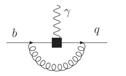
Figure 4: One particle irreducible diagram at one loop

The one particle irreducible (1PI) matrix elements can be found by evaluating the one loop diagram in Fig. 4.

The $\mathcal{O}(\alpha_{s})$ one particle irreducible correction to the operators $J_{0,j}^{(\Gamma)}=f_{j}\overline{q}\Gamma S_{j}\Psi_{v}$ (with $S_{1}=1$, $S_{2}=-\boldsymbol{\hat{\gamma}}\cdot\hat{\boldsymbol{v}}\hat{\gamma}_{0}$) is given by

$$\langle q|J_{0,j}^{(\Gamma)}|b\rangle_{\mathrm{lat,1PI}} =\alpha_{s}f_{j}\overline{u}(p^{\prime})\Sigma_{j}^{(\Gamma)}U$$

$$=\alpha_{s}\sum_{k=1,2}\xi_{jk}^{(\Gamma)}\langle q|J_{0,k}^{(\Gamma)}|b\rangle_{\mathrm{tree}}$$

$$=\alpha_{s}\sum_{k=1,2}\xi_{jk}^{(\Gamma)}f_{k}\overline{u}(p^{\prime})\Gamma S_{k}U$$ (49)

where the heavy-quark four spinor is

$$U^{(\sigma)}=\begin{pmatrix}\chi^{(\sigma)}\\ 0\end{pmatrix},\quad\text{with}\quad\chi^{(\sigma)}\in\left\{\begin{pmatrix}1\\ 0\end{pmatrix},\begin{pmatrix}0\\ 1\end{pmatrix}\right\}.$$ (50)

$\Sigma_{j}^{(\Gamma)}$ is the lattice integrand, after factoring out external quark spinors, the strong coupling constant and the velocity function $f_{j}$. To extract $\xi_{jk}^{(\Gamma)}$, we replace the spinors by Euclidean on-shell projection operators:

$$\overline{u}(p^{\prime})\mapsto\Pi_{q}(p^{\prime}) \equiv\sum_{\sigma=\uparrow,\downarrow}u^{(\sigma)}(p^{\prime})\overline{u}^{(\sigma)}(p^{\prime})=-i{p\negthickspace\negthinspace/\thickspace}^{\prime},$$

$$U\mapsto\Pi_{b} \equiv\sum_{\sigma=\uparrow,\downarrow}U^{(\sigma)}U^{(\sigma)T}=\frac{1}{2}(1+\gamma_{0})$$ (51)

and take the trace of (49):

$$f_{j}\mathrm{Tr}\left[\Pi_{q}(p^{\prime})\Sigma_{j}^{(\Gamma)}\Pi_{b}\Pi^{(\Gamma)}\right]$$

$$=\sum_{k=1,2}\xi_{jk}^{(\Gamma)}f_{k}\mathrm{Tr}\left[\Pi_{q}(p^{\prime})\Gamma S_{k}\Pi_{b}\Pi^{(\Gamma)}\right]$$ (52)

The Dirac matrix $\Pi^{(\Gamma)}$ is a suitable projection operator which depends on $\Gamma$; as both sides of (52) are a (linear) function of the four momentum $p^{\prime}$, this relation defines $\xi_{jk}^{(\Gamma)}$ for all $j,k$.

IV.8.1 Infrared subtraction function

In some configurations in momentum space the integration contour in the $k_{0}$ plane is pinched by poles. This leads to large peaks in the integrand and can generate infrared divergences in the final result.

We construct an appropriate infrared subtraction function $f^{(\mathrm{sub})}$ to smooth the integrand and thus speed up the convergence of the vegas estimate of the integral. The 1PI matrix elements can be written as

$$\xi_{jk}^{(\Gamma)} = \int\frac{d^{4}{k}}{(2\pi)^{4}}\left(f^{(\Gamma,\mathrm{lat})}_{jk}-f^{(\mathrm{sub})}_{jk}\right)+\int\frac{d^{4}{k}}{(2\pi)^{4}}f^{(\mathrm{sub})}_{jk}$$ (53)

$$= \xi^{(\Gamma,\mathrm{lat})}_{jk}+\xi^{(\mathrm{sub})}_{jk}.$$

Construction of the subtraction function is guided by the continuum integral, which has the same infrared behavior as the corresponding lattice expression. In the continuum the 1PI correction to the operator $J_{0,j}^{(\Gamma)}$ at the matching point $p^{\prime}=0$, $p=(m,0)$ is given by

$$\int\frac{d^{4}{k}}{(2\pi)^{4}}\left[\overline{u}(p^{\prime})(-igT^{a}\hat{\gamma}_{\rho})\frac{-i{k\negthickspace\negthinspace/\thickspace}}{k^{2}}f_{j}\Gamma S_{j}U\right]\times$$

$$\qquad D^{(0)}_{h}(k)(-gT^{a}v_{\rho})\frac{1}{k^{2}+\lambda^{2}}$$

$$\equiv\alpha_{s}f_{j}\;\overline{u}(p^{\prime})\Sigma_{j}^{(\Gamma,\mathrm{sub})}U$$ (54)

where $D_{h}^{(0)}(k)$ is the heavy quark propagator at $p=(m,0)$. This integral can be rendered UV finite without changing the infrared structure by replacing

$$D^{(0)}_{h}(k)=\frac{-i}{k_{0}-i\boldsymbol{v}\cdot\boldsymbol{k}}\mapsto\frac{2\gamma m}{(k+mu)^{2}+m^{2}},$$ (55)

where the metric is $g_{\mu\nu}=\operatorname{diag}(+1,+1,+1,+1)$ in Euclidean space, and the velocity four-vector is given by $u=(i\gamma,\gamma\boldsymbol{v})$. As in Eqn. (49) we write

$$f_{j}\overline{u}(p^{\prime})\Sigma_{j}^{(\Gamma,\mathrm{sub})}U =\frac{16\pi}{3}f_{j}\int\frac{d^{4}{k}}{(2\pi)^{4}}\overline{u}(p^{\prime})(-i\hat{\gamma}_{\rho})\frac{-i{k\negthickspace\negthinspace/\thickspace}}{k^{2}}\Gamma S_{j}U\frac{2\gamma m}{(k+p)^{2}+m^{2}}(-v_{\rho})\frac{1}{k^{2}+\lambda^{2}}$$

$$=\sum_{k=1,2}f_{k}\xi^{(\mathrm{sub})}_{jk}\overline{u}(p^{\prime})\Gamma S_{k}U.$$ (56)

The subtraction integral is independent of the Dirac structure and is easy to solve analytically:

$$\xi_{jk}^{(\mathrm{sub})} =\int\frac{d^{4}{k}}{(2\pi)^{4}}f^{(\mathrm{sub})}_{jk}$$

$$=-\frac{\delta_{jk}}{3\pi}\left(1+\log\lambda^{2}/m^{2}\right)+\mathcal{O}(\lambda/m).$$ (57)

This concludes our discussion of the structure of the matching calculation. In the next section we present numerical values for different quark masses and frame velocities.

V Numerical results

In Figs. 5 and 6 we show results for the matching coefficients for the vector and tensor current (see Tables 2 to 5 for numerical values).

In both cases we use a heavy mass of $m=2.8$ and a stability parameter $n=2$. These are the values currently used in nonperturbative calculations of heavy-light form factors on coarse MILC lattices Meinel et al. (2008); Liu et al. (2009). The gluon action is Symanzik improved Lepage (1994). We present results both for the ASQTad and HISQ light quark action.

For the vector current we calculate the matching coefficients for three different directions of the Lorentz index $\mu$: temporal ($\mu=0$), parallel to the frame velocity (denoted $\parallel$) and perpendicular ($\perp$). The frame velocity is chosen to be along the lattice axis $\mu=1$. For $v=0$ we consider a corresponding set of directions: $\mu=0$, $\mu=1$ and $\mu=2$.

For the tensor current there are four different cases for indices $(\mu,\nu)$: $(0,\parallel)$, $(0,\perp)$, $(\parallel,\perp)$ and $(\perp,\perp)$. For $v=0$ we choose $(\mu,\nu)=(0,1)$, $(0,2)$, $(1,2)$ and $(2,3)$. The renormalization scale of the tensor current is $\mu=m$.

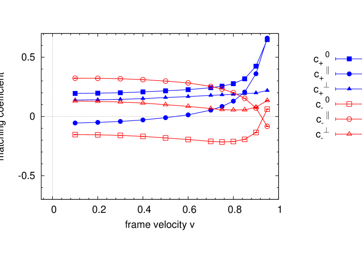
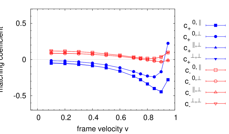
Figure 5: Matching coefficients, vector current (top) and tensor current (bottom). The heavy quark mass is $m=2.8$ and the ASQTad action is used to discretize the light quark. Due to chiral symmetry discussed in the main text the following matching coefficients are identical for the tensor current: $c_{-}^{0\parallel}$ (open red squares) and $c_{-}^{\perp\perp}$ (open red downward triangles), $c_{-}^{0\perp}$ (open red circles) and $c_{-}^{\parallel\perp}$ (open red upward triangles), $c_{+}^{0\parallel}$ (filled blue squares) and $c_{+}^{\perp\perp}$ (filled blue downward triangles), $c_{+}^{0\perp}$ (filled blue circles) and $c_{+}^{\parallel\perp}$ (filled blue upward triangles).

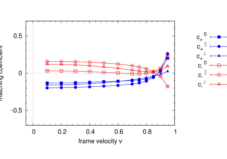
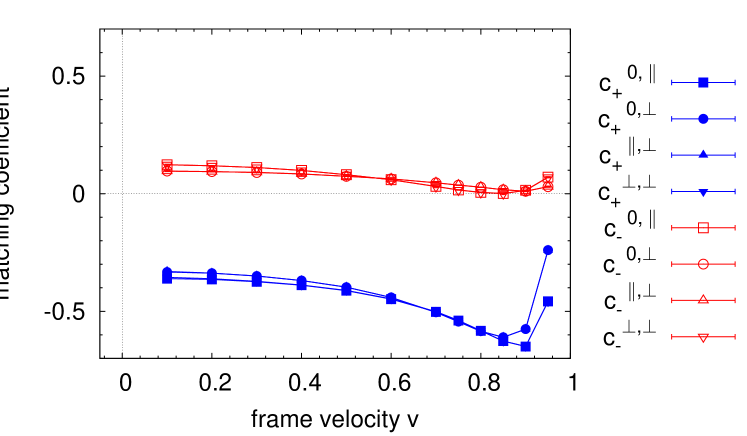
Figure 6: Matching coefficients, vector current (top) and tensor current (bottom). The heavy quark mass is $m=2.8$ and the HISQ action is used to discretize the light quark. See the comment on Fig. 5 for relations between the tensor current matching coefficients.

V.1 Discussion

As the light quark is massless its propagator and vertex functions anticommute with $\hat{\gamma}^{5}$. With $\sigma^{01}=i\hat{\gamma}^{5}\sigma^{23}$, this implies that matching coefficients for $(0,\parallel)$ and $(\perp,\perp)$ are identical (given that we boost in the direction $\mu=1$). The same holds for $(0,\perp)$ and $(\parallel,\perp)$, as $\sigma^{02}=-i\hat{\gamma}^{5}\sigma^{13}$. For $v=0$ the matching coefficients for all combinations of $(\mu,\nu)$ agree as there is no preferred direction. Heavy quark symmetry ($\hat{\gamma}^{0}\tilde{\Psi}_{v}=\tilde{\Psi}_{v}$) and relations such as $\hat{\gamma}^{0}\hat{\gamma}^{j}=-i\sigma^{0j}$ can be used to relate 1PI matrix elements of the vector and tensor current.

We emphasize that the magnitude of all matching coefficients is reduced by including mean field corrections in the renormalization parameters, the dependence on the frame velocity is weak and all matching coefficients (except for $c_{+}^{(T)}$, which depends on the renormalization scale) are of order $0.3$ or smaller for moderate $v$. With $\alpha_{s}(2/a)\approx 0.3$ the relative size of the radiative corrections does not exceed $10\%$. From heavy quark power counting we expect the matrix elements of the $O(1/m)$ operators (which are matched at tree level) to be suppressed by the same factor $\Lambda_{\mathrm{QCD}}/m\approx 0.1$ relative to the leading operators.

The matching coefficients appear to diverge for $v\rightarrow 1$. It should be noted that whereas mNRQCD reduces to NRQCD in the limit $v\rightarrow 0$, the collinear theory at $v=1$ is qualitatively different, in particular both mass and velocity renormalization are not defined in this limit.

In addition, for large $v$ the momentum distribution of the heavy quark in the initial state meson is boosted by a factor of $\gamma$ so that for highly relativistic frame velocities the power counting in $1/m$ will break down. As shown in Horgan et al. (2009) the statistical errors of nonperturbative matrix elements grow with decreasing $q^{2}$ and in practise it is unlikely that they will be calculated for $v\gtrsim 0.5$.

V.1.1 Vector current

The matching coefficient for the zero component of the vector current at $m=2.8$, $c^{(V)0}=0.04293(52)$ in Table 2, is in perfect agreement with the corresponding value $\tilde{\rho}_{0}=0.043(2)$ in Table III of Dalgic et al. (2004). For $v=0$ we find that the matching coefficients $c^{(V)1}=0.26970(40)$ and $c^{(V)2}=0.26929(39)$ agree within errors as would be expected from rotational invariance and are consistent with $\tilde{\rho}_{k}^{(0)}=0.270(1)$ in Table II of Dalgic et al. (2006).

The splitting between the matching coefficients for different Lorentz indices is reduced by using the HISQ light quark action. This reduction is not, however, as pronounced as for the tensor current. In the continuum the matching coefficient $c_{-}^{(V)}$ is zero. Using the HISQ action reduces the magnitude of $c_{-}^{(V)\parallel}$ by nearly a factor of two and an even stronger reduction is observed for $c_{-}^{(V)0}$.

V.1.2 Tensor current

For the tensor current we find that the splitting between the matching coefficients for $(\mu,\nu)=(0,\parallel)$ and $(0,\perp)$ is reduced by using the HISQ action for the light quark. A similar reduction is seen in the splitting between the $(\parallel,\perp)$ and $(\perp,\perp)$ matching coefficients.

The matching coefficients $c_{-}^{(T)\mu\nu}$ are always very small and their magnitude is about $0.1$. The size of $c_{+}^{(T)\mu\nu}$ depends on the continuum renormalization scale $\mu$; for $\mu=m$, we find that these coefficients are also very small when using ASQTad light quarks. They are, however, larger when the HISQ action is used to discretize the light quark.

V.1.3 Quark mass dependence

We repeated the calculations for a heavy quark mass $m=1.9$, which corresponds roughly to the bare quark mass on the fine MILC lattices. The results for a range of frame velocities are shown in Tables  6 to 9. The absolute size of the matching coefficients is larger than for $m=2.8$ but still typically lies in the range 0.1 - 0.5 for the frame velocities considered.

VI Conclusion

M(oving) NRQCD is a useful tool for extending the range of accessible $q^{2}$ in a lattice calculation of heavy-light form factors. The formalism has been improved and tested extensively over the last years. Radiative corrections to the effective actions have been calculated in a previous publication Horgan et al. (2009). Further reduction of systematic uncertainties is justified by an increase in precision of experimental results. In this paper we show how systematic errors due to radiative corrections can be reduced by renormalizing the heavy-light vector and tensor currents. After cancelling infrared divergences the one loop corrections to matching coefficients are of the order one and smaller. The results will be used in the current calculation of nonperturbative form factors Liu et al. (2009).

As the lattice imposes a cutoff $\sim 1/a$, operators which are formally suppressed by $1/m$ can “mix down” to the leading order operators Collins et al. (2001). These power law terms can be suppressed by constructing perturbatively subtracted $\mathcal{O}(1/m)$ operators $J^{(\Gamma)\mathrm{sub}}_{k}=J^{(\Gamma)}_{k}-\alpha_{s}\xi_{k0}^{(\Gamma)}J_{0}^{(\Gamma)}$ which do not mix down to the leading operators at one loop order. $\xi_{k0}^{(\Gamma)}$ is calculated from the one particle irreducible corrections to the $\mathcal{O}(1/m)$ operators. We find that at $v=0.4$ the non-perturbative matrix element of the subtracted $1/m$ operators is a factor of around 0.05 smaller than the leading order matrix element, which is consistent with heavy quark power counting where $\Lambda_{\mathrm{QCD}}/m\sim 0.1$. Before subtraction the ratio of the matrix elements can be as large as 0.3.

In this work we used the ASQTad and HISQ actions to discretize the light quark but it should be noted that our approach is easily extended to other discretizations such as the Domain Wall fermion action Kaplan (1992).

With currently available techniques only matrix elements of local operators in rare exclusive decays can be computed in lattice QCD. Often these operators describe the dominant effects. For the radiative decay $B\rightarrow K^{*}\gamma$ the four quark operators $Q_{3},\dots,Q_{6}$ are suppressed by their small Wilson coefficients. At the physical point where $q^{2}=0$, the contribution of $Q_{2}$ is suppressed as the $c\overline{c}$ vector resonance which connects this operator and the external photon is far off shell. Model calculations show that the matrix elements of the chromomagnetic operator $Q_{8}$ are small. This implies that the dominant contribution comes from the electromagnetic tensor operator $Q_{7}$ and the matrix elements of this operator can be evaluated in lattice QCD.

An additional complication is that the effective heavy quark theory is only valid at maximum recoil, i.e. at $q^{2}=m^{2}$. Results have to be extrapolated to $q^{2}=0$ using a phenomenological ansatz. A simple, physically motivated parametrization is given in Becirevic and Kaidalov (2000); Becirevic et al. (2007). Recently a model independent parametrization, which uses the analyticity of the form factors, has been suggested in Bailey et al. (2009).

Even if the dominant contribution to a given process is not given by a local operator, lattice calculations are still useful when combined with other approaches such as QCD sum rules.

Appendix A Pole shift

In this appendix we discuss the choice of contour for the lattice integrals. As for the self-energy calculations in Ref. Horgan et al. (2009), care has to be taken when choosing the integration contour in the $k_{0}$ plane (where $k$ is the momentum of the gluon in the loop). The heavy quark pole must lie inside the integration contour (in the $z=e^{ik_{0}}$ plane) but for certain values of the loop momentum it lies outside the unit circle. The integration contour then has to be deformed to ensure that the result can be Wick-rotated back to Minkowski space.

In the following we discuss the corresponding contour shift for the lattice three point functions. We begin by mapping the positions of the poles of the light quark propagator and then discuss the contour choice for the full integrands.

A.1 Poles of the light quark action

We use the ASQTad and HISQ actions to describe the light, relativistic quarks and, as discussed in the main text, we treat these quarks as being massless. The propagators for these actions are identical, with denominator

$$\Delta =\sum_{\nu}\sin^{2}(k_{\nu})\left(1+\frac{1}{6}\sin^{2}(k_{\nu})\right)^{2}$$

$$=\omega(1+\frac{1}{6}\omega)^{2}+s(\boldsymbol{k}),$$ (58)

where $s(\boldsymbol{k})\equiv\sum_{j=1}^{3}\sin^{2}(k_{j})\left(1+\frac{1}{6}\sin^{2}(k_{j})\right)^{2}$ and $\omega=\sin^{2}(k_{0})$.

The poles of the propagator correspond to $\Delta=0$. For given fixed, spatial three-momentum $\boldsymbol{k}$ (with $k_{j}\in[-\pi,\pi]$), finding the poles reduces to solving a cubic equation with real coefficients,

$$y^{3}-12y+36s(\boldsymbol{k})-16=0,$$ (59)

where $y=\omega+4$. This equation either has three real solutions, or one real solution and one conjugate pair of complex solutions, depending on the sign of the discriminant $D$ Bronstein et al. (1996): defined by

$$D =q^{2}-64\qquad\text{with}\quad q=18s(\boldsymbol{k})-8\;.$$ (60)

It has three real solutions if $D\leq 0$ (or equivalently $s(\boldsymbol{k})\leq 8/9$):

$$y_{1} =-2P\cos\beta, y_{2,3} =2P\cos\left(\beta\pm\frac{\pi}{3}\right)$$ (61)

where $\beta=\frac{1}{3}\arccos(q/P^{3})$ and $P=2\operatorname{sgn}q=\pm 2$.

Alternatively, it has one real solution and one conjugate pair of complex solutions if $D>0$ (or equivalently $s(\boldsymbol{k})>8/9$):

$$y_{1} =-2P\cosh\beta, y_{2,3} =P(\cosh\beta\pm i\sqrt{3}\sinh\beta)$$ (62)

where $\beta=\frac{1}{3}\operatorname{arccosh}(q/P^{3})$ and $P$ is defined as above.

In either case, for each $\omega=y-4$, there are four solutions for $z=e^{ik_{0}}$, which can be labelled as:

$$z_{\pm\pm}=\pm\sqrt{1-2\omega\pm 2\sqrt{\omega^{2}-\omega}}.$$ (63)

Of these twelve poles, two are “physical” and survive in the continuum limit. They can be identified as those that lie on the unit circle $|z|=1$ for $\boldsymbol{k}\to 0$. The other ten “spurious” poles are lattice artifacts with masses proportional to $a^{-1}$ and therefore decouple in the continuum limit. These poles (sometimes called ghost poles) are, of course, not the lattice doublers.

We calculated $z$ for a large number of random momenta $\boldsymbol{k}$ with $k_{j}\in[-\pi,\pi]$; the resulting distribution of the poles in the complex plane is shown in Fig. 7.

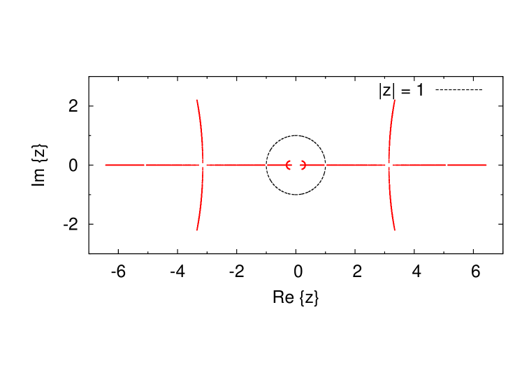
Figure 7: Poles of the massless ASQ/HISQ fermion propagator in the complex plane.

It is useful to compare the positions of these poles of the improved actions with those of the naive propagator. The equation describing the position of the poles is linear in $\omega$, leading to four solutions for $z$:

$$z^{(\mathrm{naive})}_{\pm\pm}=\pm\sqrt{1+2{\overset{\circ}{\boldsymbol{k}}}^{2}\pm 2\sqrt{{\overset{\circ}{\boldsymbol{k}}}^{2}(1+{\overset{\circ}{\boldsymbol{k}}}^{2})}}$$ (64)

with ${\overset{\circ}{\boldsymbol{k}}}^{2}=\sum_{j=1}^{3}\sin^{2}(k_{j})$. We show the comparison as a function of $|{\overset{\circ}{\boldsymbol{k}}}|$ in Fig. 8. For each spatial momentum, all the poles $z$ in the improved propagator lie outside the region defined by $|z^{(\mathrm{naive})}_{\pm+}|<|z|<|z^{(\mathrm{naive})}_{\pm-}|$. This allows us to use the positions of the naive poles as a safe lower bound for the positions of the improved poles when choosing integration contours.

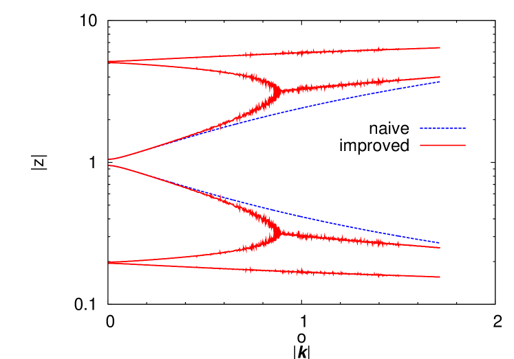
Figure 8: Absolute value of poles in the massless naive and ASQ/HISQ (improved) fermion propagator as a function of $|{\overset{\circ}{\boldsymbol{k}}}|=\sqrt{\sum_{j=1}^{3}\sin^{2}(k_{j})}$. The plot is generated by finding the poles for a large random sample of momenta $k_{j}\in[-\pi,\pi]$.

To take care of causality one can employ the $i\varepsilon$ prescription, changing the denominator to

$$\Delta=\sum_{\nu}\sin^{2}(k_{\nu})\left(1+\frac{1}{6}\sin^{2}(k_{\nu})\right)^{2}-i\varepsilon.$$ (65)

For the discussion of the effects of this, it is sufficient to concentrate on the three poles outside the unit circle with positive real part (the other poles are related to these by transformations $z\rightarrow 1/z,-z,-1/z$). One of these is the physical pole, which for $s(\boldsymbol{k})=0$ lies on the unit circle with a small negative imaginary part. In addition, there are two additional, spurious poles with larger real part: one with a negative (and small) imaginary part and one with a positive (and small) imaginary part.

The movement of these poles as the momentum increases is shown in Fig. 9. As $s(\boldsymbol{k})$ gets larger, the physical pole moves outwards. The spurious poles, meanwhile, move in opposite directions: one moves outwards just below the real axis and away from the physical pole; the other, meanwhile, moves inwards just above the real axis, towards the physical pole.

When $s(\boldsymbol{k})=8/9$, the physical pole touches (within distance $2\varepsilon$) one of the spurious poles and both, now being complex conjugates of each other, start to move away from the real axis in opposite directions.

Having established the positions of the poles, in the next section we will use these to choose the contours in the lattice integration appropriately.

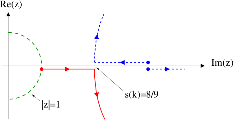
Figure 9: Movement of three of the twelve poles in the massless ASQ/HISQ propagator in the $z$ complex plane (the other poles are related by the transformations $z\rightarrow 1/z,-z,-1/z$). The arrows show the motion as $s(\boldsymbol{k})$ increases. The physical pole is shown with a solid (red) line. The spurious poles are shown using a dashed (blue) line. The unit circle is also shown (in green). The contour pinch occurs for $s(\boldsymbol{k})=8/9$.

A.2 Pole shift in one particle irreducible integrals

In this section we discuss the poles of one particle irreducible three point integrals in Sec. IV.8.

Let the position of the heavy quark pole in the $z$ plane be denoted by $z_{h}$ and the poles of the naive gluon propagator by $z_{\pm}$ such that $|z_{-}|<1<|z_{+}|$. The two poles of the naive light quark action are $z_{\pm}^{(\ell)}$, whereas the six poles of the improved light quark action are located at $z_{\pm,j}^{(\ell)}$ (and the corresponding positions with opposite sign), ordered such that

$$|z_{-,3}^{(\ell)}|<|z_{-,2}^{(\ell)}|\leq|z_{-,1}^{(\ell)}|<1<|z_{+,1}^{(\ell)}|\leq|z_{+,2}^{(\ell)}|<|z_{+,3}^{(\ell)}|\;.$$ (66)

Note that, as discussed in the previous section, only one of the poles is physical.

From the calculation of heavy quark renormalization parameters, it is known for naive (Wilson) glue that $|z_{h}|<z_{+}$ Horgan et al. (2009). The poles of the Symanzik-improved gluon action lie outside the band defined by $z_{-}<|z|<z_{+}$, so the same holds for improved gluons. We can therefore concentrate on the relative positions of the poles of the heavy and (improved) light quark propagator.

At high frame velocities and for certain choices of spatial momentum, it turns out that the heavy quark pole can cross poles of the light propagator outside the unit circle. Note, however, that as discussed in the main text, it is unlikely that very large frame velocities will be used in the evaluation of non-perturbative matrix elements. Examples are shown in Fig. 10, where we choose $\boldsymbol{k}=(x,0,0)$ with $-\pi<x\ <\pi$ and discuss both a simple action with $H_{0}$ only and the full mNRQCD action.

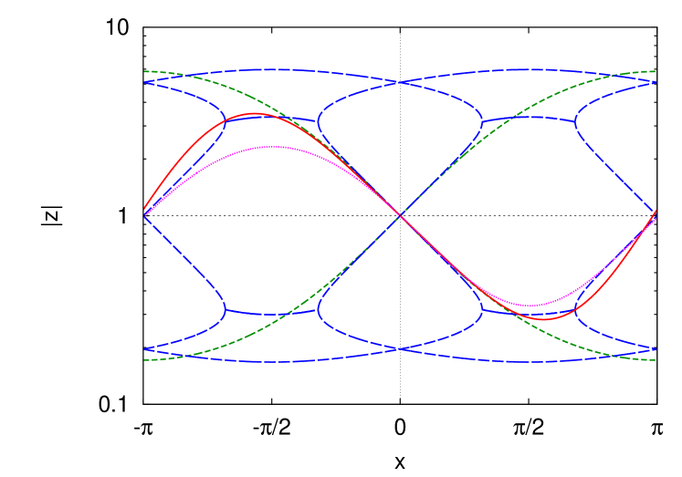
Figure 10: Absolute values of poles as a function of $x$ with $\boldsymbol{k}=(x,0,0)$. Poles of naive gluons are shown with a dashed (green) line; of improved fermions with a long dashed (blue) line; of the simple mNRQCD action ($H_{0}$ only) with a dotted (magenta) line; and of the full mNRQCD action with a solid (red) line. The frame velocity is $v=0.95$, the heavy quark mass $m=2.8$ and the stability parameter $n=2$.

The crossings are seen for certain negative values of $x$, where $|z_{+,1}^{(\ell)}|<|z_{h}|<|z_{+,2}^{(\ell)}|$. The problem gets worse if the full mNRQCD action is used. To be able to Wick-rotate back to Minkowski space in these cases, the contour needs to be deformed such that it encloses the heavy quark pole but not the light quark poles outside the unit circle. Suitable contours are shown on the left in Fig. 11. In a similar way to that used in Ref. Hart et al. (2007), the contours can be deformed to avoid the poles as much as possible, arising at the triple contours shown on the right in Fig. 11.

Computationally, the procedure is as follows. We choose the contour(s) separately for each value of the spatial momentum (generated, for instance, by the vegas integration code):

1. $|z_{h}|<z_{-},|z_{-,1}^{(\ell)}|$: As $z_{h}$ is not the smallest negative pole and the contour does not need to be shifted from $|z|=1$.

2. $z_{-},|z_{-,1}^{(\ell)}|<|z_{h}|<z_{+},|z_{+,1}^{(\ell)}|$. The contour is shifted outwards to halfway between $|z_{h}|$ and $\min\{z_{+},z_{+,1}^{(\ell)}\}$.

3. $|z_{+,j}^{(\ell)}|<|z_{h}|<|z_{+,j+1}^{(\ell)}|,z_{+}$ for $j=1,2$ (see Fig. 10). A pole crossing has occurred and it is necessary to integrate along three contours: (a) anticlockwise without shift, $|z|=1$; (b) clockwise, shifting the contour midway between $|z_{+,j}^{(\ell)}|$ and $|z_{h}|$; and (c) counterclockwise with the contour between $|z_{h}|$ and $\min\{|z_{+,j+1}^{(\ell)}|,z_{+}\}$.

To speed up the vegas calculation, in cases (1) and (2) we first check using the poles of the naive light quark action, only calculating the poles of the improved version if that test is inconclusive. When shifting a contour midway between poles $z_{a}$ and $z_{b}$, we shift the contour to $\sqrt{z_{a}z_{b}}$.

As the pole crossing only occurs for large momenta this is a lattice artifact which would disappear in the continuum limit. It must, however, be included in a lattice–continuum matching calculation.

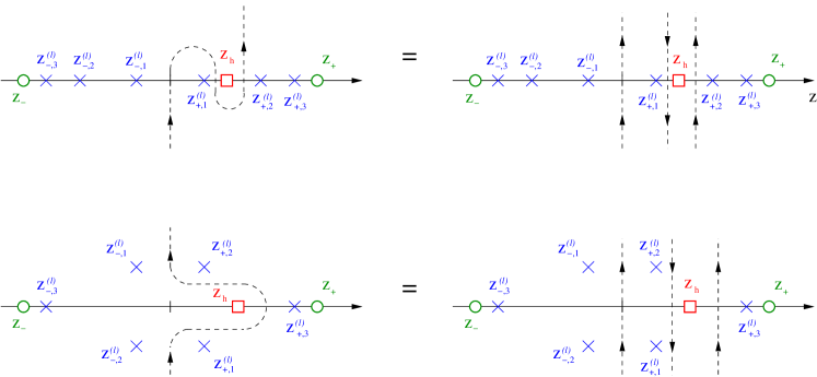
Figure 11: Integration contour for momentum space configurations with pole crossing. The light quark poles are denoted by $\times$, the naive gluon poles by $\circ$ and the heavy quark pole by $\square$.

$v$	$c^{(V)0}$	$c^{(V)1}$	$c^{(V)2}$
$0.00$	${\color[rgb]{1,1,1}{-}}0.04293(52)$	${\color[rgb]{1,1,1}{-}}0.26970(40)$	${\color[rgb]{1,1,1}{-}}0.26929(39)$

$v$	$c_{+}^{(V)0}$	$c_{+}^{(V)\parallel}$	$c_{+}^{(V)\perp}$
$0.10$	${\color[rgb]{1,1,1}{-}}0.1945(21)$	$-0.0553(22)$	${\color[rgb]{1,1,1}{-}}0.1384(18)$
$0.20$	${\color[rgb]{1,1,1}{-}}0.1965(12)$	$-0.0500(13)$	${\color[rgb]{1,1,1}{-}}0.1411(12)$
$0.30$	${\color[rgb]{1,1,1}{-}}0.2005(10)$	$-0.0419(11)$	${\color[rgb]{1,1,1}{-}}0.1444(10)$
$0.40$	${\color[rgb]{1,1,1}{-}}0.20708(84)$	$-0.0293(10)$	${\color[rgb]{1,1,1}{-}}0.15071(88)$
$0.50$	${\color[rgb]{1,1,1}{-}}0.21660(77)$	$-0.01038(88)$	${\color[rgb]{1,1,1}{-}}0.15972(84)$
$0.60$	${\color[rgb]{1,1,1}{-}}0.22620(73)$	${\color[rgb]{1,1,1}{-}}0.01358(85)$	${\color[rgb]{1,1,1}{-}}0.16775(85)$
$0.70$	${\color[rgb]{1,1,1}{-}}0.24297(71)$	${\color[rgb]{1,1,1}{-}}0.05349(80)$	${\color[rgb]{1,1,1}{-}}0.17817(87)$
$0.75$	${\color[rgb]{1,1,1}{-}}0.25596(72)$	${\color[rgb]{1,1,1}{-}}0.08412(80)$	${\color[rgb]{1,1,1}{-}}0.18243(91)$
$0.80$	${\color[rgb]{1,1,1}{-}}0.27674(77)$	${\color[rgb]{1,1,1}{-}}0.12920(85)$	${\color[rgb]{1,1,1}{-}}0.1862(10)$
$0.85$	${\color[rgb]{1,1,1}{-}}0.3179(13)$	${\color[rgb]{1,1,1}{-}}0.2057(13)$	${\color[rgb]{1,1,1}{-}}0.1918(12)$
$0.90$	${\color[rgb]{1,1,1}{-}}0.4244(15)$	${\color[rgb]{1,1,1}{-}}0.3604(16)$	${\color[rgb]{1,1,1}{-}}0.1986(15)$
$0.95$	${\color[rgb]{1,1,1}{-}}0.6492(19)$	${\color[rgb]{1,1,1}{-}}0.6615(19)$	${\color[rgb]{1,1,1}{-}}0.2186(23)$

$v$	$c_{-}^{(V)0}$	$c_{-}^{(V)\parallel}$	$c_{-}^{(V)\perp}$
$0.10$	$-0.1533(22)$	${\color[rgb]{1,1,1}{-}}0.3227(22)$	${\color[rgb]{1,1,1}{-}}0.1301(17)$
$0.20$	$-0.1547(13)$	${\color[rgb]{1,1,1}{-}}0.3220(13)$	${\color[rgb]{1,1,1}{-}}0.1274(10)$
$0.30$	$-0.1598(10)$	${\color[rgb]{1,1,1}{-}}0.3183(10)$	${\color[rgb]{1,1,1}{-}}0.12224(81)$
$0.40$	$-0.16838(86)$	${\color[rgb]{1,1,1}{-}}0.31106(85)$	${\color[rgb]{1,1,1}{-}}0.11325(72)$
$0.50$	$-0.18137(81)$	${\color[rgb]{1,1,1}{-}}0.29887(80)$	${\color[rgb]{1,1,1}{-}}0.09967(67)$
$0.60$	$-0.19460(80)$	${\color[rgb]{1,1,1}{-}}0.28291(80)$	${\color[rgb]{1,1,1}{-}}0.08532(68)$
$0.70$	$-0.21033(81)$	${\color[rgb]{1,1,1}{-}}0.25390(80)$	${\color[rgb]{1,1,1}{-}}0.06649(69)$
$0.75$	$-0.21513(84)$	${\color[rgb]{1,1,1}{-}}0.23150(83)$	${\color[rgb]{1,1,1}{-}}0.05808(73)$
$0.80$	$-0.21139(91)$	${\color[rgb]{1,1,1}{-}}0.20128(91)$	${\color[rgb]{1,1,1}{-}}0.05445(80)$
$0.85$	$-0.1931(11)$	${\color[rgb]{1,1,1}{-}}0.1530(12)$	${\color[rgb]{1,1,1}{-}}0.0561(10)$
$0.90$	$-0.1353(13)$	${\color[rgb]{1,1,1}{-}}0.0713(14)$	${\color[rgb]{1,1,1}{-}}0.0777(12)$
$0.95$	${\color[rgb]{1,1,1}{-}}0.0615(23)$	$-0.0832(23)$	${\color[rgb]{1,1,1}{-}}0.1347(22)$

Table 2: Vector current matching coefficients for heavy quark mass $m=2.8$. The ASQTad action is used to discretize the light quark. The Lorentz indices can be timelike ($0$), parallel ($\parallel$) or perpendicular ($\perp$) to the frame velocity. The table shows the central value and error from the vegas integration.

$v$	$c^{(T)0,1}$	$c^{(T)0,2}$	$c^{(T)1,2}$	$c^{(T)2,3}$
$0.00$	${\color[rgb]{1,1,1}{-}}0.0762(12)$	${\color[rgb]{1,1,1}{-}}0.0761(12)$	${\color[rgb]{1,1,1}{-}}0.0763(12)$	${\color[rgb]{1,1,1}{-}}0.0761(12)$

$v$	$c_{+}^{(T)0,\parallel}$	$c_{+}^{(T)0,\perp}$	$c_{+}^{(T)\parallel,\perp}$	$c_{+}^{(T)\perp,\perp}$
$0.10$	$-0.0507(24)$	$-0.0159(21)$	$-0.0157(22)$	$-0.0463(24)$
$0.20$	$-0.0559(17)$	$-0.0206(16)$	$-0.0214(16)$	$-0.0526(17)$
$0.30$	$-0.0675(16)$	$-0.0325(15)$	$-0.0321(15)$	$-0.0652(16)$
$0.40$	$-0.0861(15)$	$-0.0496(15)$	$-0.0497(15)$	$-0.0846(15)$
$0.50$	$-0.1148(16)$	$-0.0748(15)$	$-0.0750(15)$	$-0.1136(16)$
$0.60$	$-0.1605(17)$	$-0.1135(16)$	$-0.1136(16)$	$-0.1595(17)$
$0.70$	$-0.2302(19)$	$-0.1666(18)$	$-0.1668(18)$	$-0.2295(19)$
$0.75$	$-0.2791(21)$	$-0.1984(21)$	$-0.1992(21)$	$-0.2782(21)$
$0.80$	$-0.3379(26)$	$-0.2280(25)$	$-0.2292(25)$	$-0.3368(26)$
$0.85$	$-0.4006(34)$	$-0.2397(35)$	$-0.2397(35)$	$-0.3990(34)$
$0.90$	$-0.4463(53)$	$-0.1688(53)$	$-0.1696(53)$	$-0.4441(53)$
$0.95$	$-0.279(14)$	${\color[rgb]{1,1,1}{-}}0.224(14)$	${\color[rgb]{1,1,1}{-}}0.223(14)$	$-0.279(14)$

$v$	$c_{-}^{(T)0,\parallel}$	$c_{-}^{(T)0,\perp}$	$c_{-}^{(T)\parallel,\perp}$	$c_{-}^{(T)\perp,\perp}$
$0.10$	${\color[rgb]{1,1,1}{-}}0.1184(20)$	${\color[rgb]{1,1,1}{-}}0.0849(18)$	${\color[rgb]{1,1,1}{-}}0.0871(18)$	${\color[rgb]{1,1,1}{-}}0.1189(20)$
$0.20$	${\color[rgb]{1,1,1}{-}}0.1147(11)$	${\color[rgb]{1,1,1}{-}}0.0839(11)$	${\color[rgb]{1,1,1}{-}}0.0855(11)$	${\color[rgb]{1,1,1}{-}}0.1149(11)$
$0.30$	${\color[rgb]{1,1,1}{-}}0.10781(85)$	${\color[rgb]{1,1,1}{-}}0.07967(86)$	${\color[rgb]{1,1,1}{-}}0.08054(86)$	${\color[rgb]{1,1,1}{-}}0.10774(85)$
$0.40$	${\color[rgb]{1,1,1}{-}}0.09607(74)$	${\color[rgb]{1,1,1}{-}}0.07144(76)$	${\color[rgb]{1,1,1}{-}}0.07214(77)$	${\color[rgb]{1,1,1}{-}}0.09583(74)$
$0.50$	${\color[rgb]{1,1,1}{-}}0.07857(69)$	${\color[rgb]{1,1,1}{-}}0.05896(72)$	${\color[rgb]{1,1,1}{-}}0.05912(72)$	${\color[rgb]{1,1,1}{-}}0.07848(69)$
$0.60$	${\color[rgb]{1,1,1}{-}}0.05889(69)$	${\color[rgb]{1,1,1}{-}}0.04414(72)$	${\color[rgb]{1,1,1}{-}}0.04412(72)$	${\color[rgb]{1,1,1}{-}}0.05860(69)$
$0.70$	${\color[rgb]{1,1,1}{-}}0.03355(70)$	${\color[rgb]{1,1,1}{-}}0.02162(73)$	${\color[rgb]{1,1,1}{-}}0.02142(73)$	${\color[rgb]{1,1,1}{-}}0.03332(70)$
$0.75$	${\color[rgb]{1,1,1}{-}}0.02163(74)$	${\color[rgb]{1,1,1}{-}}0.00812(77)$	${\color[rgb]{1,1,1}{-}}0.00787(76)$	${\color[rgb]{1,1,1}{-}}0.02131(74)$
$0.80$	${\color[rgb]{1,1,1}{-}}0.01460(82)$	$-0.00494(84)$	$-0.00522(84)$	${\color[rgb]{1,1,1}{-}}0.01425(82)$
$0.85$	${\color[rgb]{1,1,1}{-}}0.0146(10)$	$-0.0199(10)$	$-0.0205(10)$	${\color[rgb]{1,1,1}{-}}0.0142(10)$
$0.90$	${\color[rgb]{1,1,1}{-}}0.0361(13)$	$-0.0310(13)$	$-0.0312(13)$	${\color[rgb]{1,1,1}{-}}0.0357(13)$
$0.95$	${\color[rgb]{1,1,1}{-}}0.0980(22)$	$-0.0125(22)$	$-0.0114(22)$	${\color[rgb]{1,1,1}{-}}0.0976(22)$

Table 3: Tensor current matching coefficients for heavy quark mass $m=2.8$. The ASQTad action is used to discretize the light quark.

$v$	$c^{(V)0}$	$c^{(V)1}$	$c^{(V)2}$
$0.00$	$-0.10173(91)$	$-0.03811(87)$	$-0.03825(87)$

$v$	$c_{+}^{(V)0}$	$c_{+}^{(V)\parallel}$	$c_{+}^{(V)\perp}$
$0.10$	$-0.1323(22)$	$-0.1980(22)$	$-0.1593(20)$
$0.20$	$-0.1318(15)$	$-0.1942(15)$	$-0.1575(14)$
$0.30$	$-0.1286(13)$	$-0.1902(13)$	$-0.1513(12)$
$0.40$	$-0.1226(12)$	$-0.1835(12)$	$-0.1417(12)$
$0.50$	$-0.1147(11)$	$-0.1732(12)$	$-0.1276(11)$
$0.60$	$-0.1079(11)$	$-0.1636(11)$	$-0.1116(11)$
$0.70$	$-0.0982(11)$	$-0.1454(11)$	$-0.0895(11)$
$0.75$	$-0.0906(11)$	$-0.1307(11)$	$-0.0760(12)$
$0.80$	$-0.0775(11)$	$-0.1067(11)$	$-0.0610(12)$
$0.85$	$-0.0465(12)$	$-0.0578(12)$	$-0.0412(14)$
$0.90$	${\color[rgb]{1,1,1}{-}}0.0268(13)$	${\color[rgb]{1,1,1}{-}}0.0411(14)$	$-0.0157(16)$
$0.95$	${\color[rgb]{1,1,1}{-}}0.2011(22)$	${\color[rgb]{1,1,1}{-}}0.2624(21)$	${\color[rgb]{1,1,1}{-}}0.0229(23)$

$v$	$c_{-}^{(V)0}$	$c_{-}^{(V)\parallel}$	$c_{-}^{(V)\perp}$
$0.10$	${\color[rgb]{1,1,1}{-}}0.0322(21)$	${\color[rgb]{1,1,1}{-}}0.1574(20)$	${\color[rgb]{1,1,1}{-}}0.1218(16)$
$0.20$	${\color[rgb]{1,1,1}{-}}0.0303(13)$	${\color[rgb]{1,1,1}{-}}0.1562(12)$	${\color[rgb]{1,1,1}{-}}0.1183(10)$
$0.30$	${\color[rgb]{1,1,1}{-}}0.0269(10)$	${\color[rgb]{1,1,1}{-}}0.15322(93)$	${\color[rgb]{1,1,1}{-}}0.11199(78)$
$0.40$	${\color[rgb]{1,1,1}{-}}0.02062(84)$	${\color[rgb]{1,1,1}{-}}0.14692(82)$	${\color[rgb]{1,1,1}{-}}0.10099(70)$
$0.50$	${\color[rgb]{1,1,1}{-}}0.01122(78)$	${\color[rgb]{1,1,1}{-}}0.13632(76)$	${\color[rgb]{1,1,1}{-}}0.08488(66)$
$0.60$	${\color[rgb]{1,1,1}{-}}0.00253(77)$	${\color[rgb]{1,1,1}{-}}0.12358(76)$	${\color[rgb]{1,1,1}{-}}0.06641(67)$
$0.70$	$-0.00754(78)$	${\color[rgb]{1,1,1}{-}}0.10023(77)$	${\color[rgb]{1,1,1}{-}}0.04171(68)$
$0.75$	$-0.00961(81)$	${\color[rgb]{1,1,1}{-}}0.08269(80)$	${\color[rgb]{1,1,1}{-}}0.02950(72)$
$0.80$	$-0.00407(88)$	${\color[rgb]{1,1,1}{-}}0.05947(88)$	${\color[rgb]{1,1,1}{-}}0.02188(79)$
$0.85$	${\color[rgb]{1,1,1}{-}}0.0132(10)$	${\color[rgb]{1,1,1}{-}}0.0209(10)$	${\color[rgb]{1,1,1}{-}}0.01954(93)$
$0.90$	${\color[rgb]{1,1,1}{-}}0.0648(13)$	$-0.0436(13)$	${\color[rgb]{1,1,1}{-}}0.0357(12)$
$0.95$	${\color[rgb]{1,1,1}{-}}0.2373(22)$	$-0.1771(23)$	${\color[rgb]{1,1,1}{-}}0.0933(22)$

Table 4: Vector current matching coefficients for heavy quark mass $m=2.8$. The HISQ action is used to discretize the light quark.

$v$	$c^{(T)0,1}$	$c^{(T)0,2}$	$c^{(T)1,2}$	$c^{(T)2,3}$
$0.00$	$-0.2317(15)$	$-0.2318(15)$	$-0.2316(15)$	$-0.2317(15)$

$v$	$c_{+}^{(T)0,\parallel}$	$c_{+}^{(T)0,\perp}$	$c_{+}^{(T)\parallel,\perp}$	$c_{+}^{(T)\perp,\perp}$
$0.10$	$-0.3610(25)$	$-0.3330(23)$	$-0.3305(23)$	$-0.3555(25)$
$0.20$	$-0.3643(19)$	$-0.3380(18)$	$-0.3375(18)$	$-0.3614(19)$
$0.30$	$-0.3741(17)$	$-0.3500(17)$	$-0.3496(17)$	$-0.3726(17)$
$0.40$	$-0.3890(17)$	$-0.3691(17)$	$-0.3690(17)$	$-0.3881(17)$
$0.50$	$-0.4120(17)$	$-0.3974(17)$	$-0.3970(17)$	$-0.4109(17)$
$0.60$	$-0.4480(18)$	$-0.4410(18)$	$-0.4414(18)$	$-0.4469(18)$
$0.70$	$-0.5022(21)$	$-0.5040(20)$	$-0.5043(20)$	$-0.5011(21)$
$0.75$	$-0.5394(23)$	$-0.5437(22)$	$-0.5441(22)$	$-0.5384(23)$
$0.80$	$-0.5829(27)$	$-0.5843(26)$	$-0.5854(26)$	$-0.5827(27)$
$0.85$	$-0.6264(35)$	$-0.6102(34)$	$-0.6103(34)$	$-0.6264(35)$
$0.90$	$-0.6497(53)$	$-0.5754(53)$	$-0.5761(53)$	$-0.6490(53)$
$0.95$	$-0.458(14)$	$-0.240(14)$	$-0.240(14)$	$-0.459(14)$

$v$	$c_{-}^{(T)0,\parallel}$	$c_{-}^{(T)0,\perp}$	$c_{-}^{(T)\parallel,\perp}$	$c_{-}^{(T)\perp,\perp}$
$0.10$	${\color[rgb]{1,1,1}{-}}0.1230(19)$	${\color[rgb]{1,1,1}{-}}0.0964(17)$	${\color[rgb]{1,1,1}{-}}0.0955(18)$	${\color[rgb]{1,1,1}{-}}0.1234(19)$
$0.20$	${\color[rgb]{1,1,1}{-}}0.1187(11)$	${\color[rgb]{1,1,1}{-}}0.0939(11)$	${\color[rgb]{1,1,1}{-}}0.0938(11)$	${\color[rgb]{1,1,1}{-}}0.1187(11)$
$0.30$	${\color[rgb]{1,1,1}{-}}0.11138(82)$	${\color[rgb]{1,1,1}{-}}0.09018(84)$	${\color[rgb]{1,1,1}{-}}0.09064(84)$	${\color[rgb]{1,1,1}{-}}0.11126(82)$
$0.40$	${\color[rgb]{1,1,1}{-}}0.09914(72)$	${\color[rgb]{1,1,1}{-}}0.08398(75)$	${\color[rgb]{1,1,1}{-}}0.08432(75)$	${\color[rgb]{1,1,1}{-}}0.09898(72)$
$0.50$	${\color[rgb]{1,1,1}{-}}0.08099(67)$	${\color[rgb]{1,1,1}{-}}0.07380(70)$	${\color[rgb]{1,1,1}{-}}0.07417(70)$	${\color[rgb]{1,1,1}{-}}0.08075(67)$
$0.60$	${\color[rgb]{1,1,1}{-}}0.05968(67)$	${\color[rgb]{1,1,1}{-}}0.06302(70)$	${\color[rgb]{1,1,1}{-}}0.06342(70)$	${\color[rgb]{1,1,1}{-}}0.05937(67)$
$0.70$	${\color[rgb]{1,1,1}{-}}0.03107(68)$	${\color[rgb]{1,1,1}{-}}0.04637(71)$	${\color[rgb]{1,1,1}{-}}0.04668(71)$	${\color[rgb]{1,1,1}{-}}0.03060(68)$
$0.75$	${\color[rgb]{1,1,1}{-}}0.01635(73)$	${\color[rgb]{1,1,1}{-}}0.03647(75)$	${\color[rgb]{1,1,1}{-}}0.03669(75)$	${\color[rgb]{1,1,1}{-}}0.01583(72)$
$0.80$	${\color[rgb]{1,1,1}{-}}0.00591(80)$	${\color[rgb]{1,1,1}{-}}0.02745(82)$	${\color[rgb]{1,1,1}{-}}0.02778(82)$	${\color[rgb]{1,1,1}{-}}0.00529(80)$
$0.85$	${\color[rgb]{1,1,1}{-}}0.00098(94)$	${\color[rgb]{1,1,1}{-}}0.0168(10)$	${\color[rgb]{1,1,1}{-}}0.0169(10)$	${\color[rgb]{1,1,1}{-}}0.00026(94)$
$0.90$	${\color[rgb]{1,1,1}{-}}0.0146(12)$	${\color[rgb]{1,1,1}{-}}0.0102(12)$	${\color[rgb]{1,1,1}{-}}0.0108(12)$	${\color[rgb]{1,1,1}{-}}0.0141(12)$
$0.95$	${\color[rgb]{1,1,1}{-}}0.0705(22)$	${\color[rgb]{1,1,1}{-}}0.0299(22)$	${\color[rgb]{1,1,1}{-}}0.0302(22)$	${\color[rgb]{1,1,1}{-}}0.0696(22)$

Table 5: Tensor current matching coefficients for heavy quark mass $m=2.8$. The HISQ action is used to discretize the light quark.

$v$	$c^{(V)0}$	$c^{(V)1}$	$c^{(V)2}$
$0.00$	$-0.06534(59)$	${\color[rgb]{1,1,1}{-}}0.33741(41)$	${\color[rgb]{1,1,1}{-}}0.33681(41)$

$v$	$c_{+}^{(V)0}$	$c_{+}^{(V)\parallel}$	$c_{+}^{(V)\perp}$
$0.01$	${\color[rgb]{1,1,1}{-}}0.246(18)$	$-0.185(18)$	${\color[rgb]{1,1,1}{-}}0.162(14)$
$0.10$	${\color[rgb]{1,1,1}{-}}0.2164(21)$	$-0.1954(22)$	${\color[rgb]{1,1,1}{-}}0.1514(18)$
$0.20$	${\color[rgb]{1,1,1}{-}}0.2147(13)$	$-0.1924(14)$	${\color[rgb]{1,1,1}{-}}0.1501(12)$
$0.30$	${\color[rgb]{1,1,1}{-}}0.2170(10)$	$-0.1849(12)$	${\color[rgb]{1,1,1}{-}}0.1506(10)$

$v$	$c_{-}^{(V)0}$	$c_{-}^{(V)\parallel}$	$c_{-}^{(V)\perp}$
$0.01$	$-0.294(18)$	${\color[rgb]{1,1,1}{-}}0.530(18)$	${\color[rgb]{1,1,1}{-}}0.185(14)$
$0.10$	$-0.2831(21)$	${\color[rgb]{1,1,1}{-}}0.5337(22)$	${\color[rgb]{1,1,1}{-}}0.1848(17)$
$0.20$	$-0.2829(13)$	${\color[rgb]{1,1,1}{-}}0.5353(13)$	${\color[rgb]{1,1,1}{-}}0.1847(11)$
$0.30$	$-0.2889(11)$	${\color[rgb]{1,1,1}{-}}0.5333(11)$	${\color[rgb]{1,1,1}{-}}0.18050(89)$

Table 6: Vector current matching coefficients for heavy quark mass $m=1.9$. The ASQTad action is used to discretize the light quark.

$v$	$c^{(T)0,1}$	$c^{(T)0,2}$	$c^{(T)1,2}$	$c^{(T)2,3}$
$0.00$	${\color[rgb]{1,1,1}{-}}0.3410(16)$	${\color[rgb]{1,1,1}{-}}0.3411(16)$	${\color[rgb]{1,1,1}{-}}0.3414(16)$	${\color[rgb]{1,1,1}{-}}0.3412(16)$

$v$	$c_{+}^{(T)0,\parallel}$	$c_{+}^{(T)0,\perp}$	$c_{+}^{(T)\parallel,\perp}$	$c_{+}^{(T)\perp,\perp}$
$0.01$	${\color[rgb]{1,1,1}{-}}0.141(18)$	${\color[rgb]{1,1,1}{-}}0.210(14)$	${\color[rgb]{1,1,1}{-}}0.205(14)$	${\color[rgb]{1,1,1}{-}}0.167(18)$
$0.10$	${\color[rgb]{1,1,1}{-}}0.1524(26)$	${\color[rgb]{1,1,1}{-}}0.2094(24)$	${\color[rgb]{1,1,1}{-}}0.2085(24)$	${\color[rgb]{1,1,1}{-}}0.1577(26)$
$0.20$	${\color[rgb]{1,1,1}{-}}0.1448(21)$	${\color[rgb]{1,1,1}{-}}0.2017(20)$	${\color[rgb]{1,1,1}{-}}0.2017(20)$	${\color[rgb]{1,1,1}{-}}0.1476(21)$
$0.30$	${\color[rgb]{1,1,1}{-}}0.1319(19)$	${\color[rgb]{1,1,1}{-}}0.1907(18)$	${\color[rgb]{1,1,1}{-}}0.1903(18)$	${\color[rgb]{1,1,1}{-}}0.1339(19)$

$v$	$c_{-}^{(T)0,\parallel}$	$c_{-}^{(T)0,\perp}$	$c_{-}^{(T)\parallel,\perp}$	$c_{-}^{(T)\perp,\perp}$
$0.01$	${\color[rgb]{1,1,1}{-}}0.162(18)$	${\color[rgb]{1,1,1}{-}}0.119(14)$	${\color[rgb]{1,1,1}{-}}0.119(14)$	${\color[rgb]{1,1,1}{-}}0.190(18)$
$0.10$	${\color[rgb]{1,1,1}{-}}0.1784(20)$	${\color[rgb]{1,1,1}{-}}0.1268(18)$	${\color[rgb]{1,1,1}{-}}0.1285(18)$	${\color[rgb]{1,1,1}{-}}0.1814(20)$
$0.20$	${\color[rgb]{1,1,1}{-}}0.1777(12)$	${\color[rgb]{1,1,1}{-}}0.1267(12)$	${\color[rgb]{1,1,1}{-}}0.1273(12)$	${\color[rgb]{1,1,1}{-}}0.1785(12)$
$0.30$	${\color[rgb]{1,1,1}{-}}0.1712(10)$	${\color[rgb]{1,1,1}{-}}0.12228(94)$	${\color[rgb]{1,1,1}{-}}0.12256(94)$	${\color[rgb]{1,1,1}{-}}0.17183(95)$

Table 7: Tensor current matching coefficients for heavy quark mass $m=1.9$. The ASQTad action is used to discretize the light quark.

$v$	$c^{(V)0}$	$c^{(V)1}$	$c^{(V)2}$
$0.00$	$-0.15556(94)$	${\color[rgb]{1,1,1}{-}}0.01365(88)$	${\color[rgb]{1,1,1}{-}}0.01296(88)$

$v$	$c_{+}^{(V)0}$	$c_{+}^{(V)\parallel}$	$c_{+}^{(V)\perp}$
$0.01$	$-0.095(17)$	$-0.273(17)$	$-0.164(13)$
$0.10$	$-0.1180(23)$	$-0.2782(22)$	$-0.1721(20)$
$0.20$	$-0.1198(16)$	$-0.2779(16)$	$-0.1720(15)$
$0.30$	$-0.1176(13)$	$-0.2744(14)$	$-0.1689(13)$

$v$	$c_{-}^{(V)0}$	$c_{-}^{(V)\parallel}$	$c_{-}^{(V)\perp}$
$0.01$	$-0.055(17)$	${\color[rgb]{1,1,1}{-}}0.283(17)$	${\color[rgb]{1,1,1}{-}}0.189(13)$
$0.10$	$-0.0359(21)$	${\color[rgb]{1,1,1}{-}}0.2908(21)$	${\color[rgb]{1,1,1}{-}}0.1840(17)$
$0.20$	$-0.0366(13)$	${\color[rgb]{1,1,1}{-}}0.2926(13)$	${\color[rgb]{1,1,1}{-}}0.1831(11)$
$0.30$	$-0.0415(10)$	${\color[rgb]{1,1,1}{-}}0.2914(10)$	${\color[rgb]{1,1,1}{-}}0.17766(88)$

Table 8: Vector current matching coefficients for heavy quark mass $m=1.9$. The HISQ action is used to discretize the light quark.

$v$	$c^{(T)0,1}$	$c^{(T)0,2}$	$c^{(T)1,2}$	$c^{(T)2,3}$
$0.00$	${\color[rgb]{1,1,1}{-}}0.0171(17)$	${\color[rgb]{1,1,1}{-}}0.0175(17)$	${\color[rgb]{1,1,1}{-}}0.0172(17)$	${\color[rgb]{1,1,1}{-}}0.0173(17)$

$v$	$c_{+}^{(T)0,\parallel}$	$c_{+}^{(T)0,\perp}$	$c_{+}^{(T)\parallel,\perp}$	$c_{+}^{(T)\perp,\perp}$
$0.01$	$-0.199(17)$	$-0.123(13)$	$-0.112(13)$	$-0.174(17)$
$0.10$	$-0.1800(27)$	$-0.1163(25)$	$-0.1150(25)$	$-0.1763(27)$
$0.20$	$-0.1863(22)$	$-0.1231(21)$	$-0.1229(21)$	$-0.1840(22)$
$0.30$	$-0.1966(20)$	$-0.1347(20)$	$-0.1345(20)$	$-0.1950(20)$

$v$	$c_{-}^{(T)0,\parallel}$	$c_{-}^{(T)0,\perp}$	$c_{-}^{(T)\parallel,\perp}$	$c_{-}^{(T)\perp,\perp}$
$0.01$	${\color[rgb]{1,1,1}{-}}0.208(17)$	${\color[rgb]{1,1,1}{-}}0.135(13)$	${\color[rgb]{1,1,1}{-}}0.125(14)$	${\color[rgb]{1,1,1}{-}}0.183(17)$
$0.10$	${\color[rgb]{1,1,1}{-}}0.1915(19)$	${\color[rgb]{1,1,1}{-}}0.1285(17)$	${\color[rgb]{1,1,1}{-}}0.1287(18)$	${\color[rgb]{1,1,1}{-}}0.1889(19)$
$0.20$	${\color[rgb]{1,1,1}{-}}0.1889(12)$	${\color[rgb]{1,1,1}{-}}0.1282(12)$	${\color[rgb]{1,1,1}{-}}0.1287(12)$	${\color[rgb]{1,1,1}{-}}0.1876(12)$
$0.30$	${\color[rgb]{1,1,1}{-}}0.18199(93)$	${\color[rgb]{1,1,1}{-}}0.12518(94)$	${\color[rgb]{1,1,1}{-}}0.12555(94)$	${\color[rgb]{1,1,1}{-}}0.18114(93)$

Table 9: Tensor current matching coefficients for heavy quark mass $am=1.9$. The HISQ action is used to discretize the light quark.