Rigorous coherent-structure theory for falling liquid films: Viscous dispersion effects on bound-state formation and self-organization

Abstract

We examine the interaction of two-dimensional solitary pulses on falling liquid films. We make use of the second-order model derived by Ruyer-Quil and Manneville [Eur. Phys. J. B 6, 277 (1998); Eur. Phys. J. B 15, 357 (2000); Phys. Fluids 14, 170 (2002)] by combining the long-wave approximation with a weighted residuals technique. The model includes (second-order) viscous dispersion effects which originate from the streamwise momentum equation and tangential stress balance. These effects play a dispersive role that primarily influences the shape of the capillary ripples in front of the solitary pulses. We show that different physical parameters, such as surface tension and viscosity, play a crucial role in the interaction between solitary pulses giving rise eventually to the formation of bound states consisting of two or more pulses separated by well-defined distances and travelling at the same velocity. By developing a rigorous coherent-structure theory, we are able to theoretically predict the pulse-separation distances for which bound states are formed. Viscous dispersion affects the distances at which bound states are observed. We show that the theory is in very good agreement with computations of the second-order model. We also demonstrate that the presence of bound states allows the film free surface to reach a self-organized state that can be statistically described in terms of a gas of solitary waves separated by a typical mean distance and characterized by a typical density.

I Introduction

The dynamics of a liquid film falling down a vertical wall has been the subject of numerous studies since the pioneering works by the father-son Kapitza team Kapitza (1948a, b); Kapitza and Kapitza (1949). Wave evolution on a falling film is a classical long-wave hydrodynamic instability with a rich variety of spatial and temporal structures and a rich spectrum of wave forms and wave transitions, starting from nearly harmonic waves at the inlet to complex spatio-temporal highly nonlinear wave patterns downstream. Such patterns are known to profoundly affect the heat and mass transfer of multi-phase industrial units. Reviews of the dynamics of a falling film are given in Refs. Chang, 1994; Chang and Demekhin, 2002; Kalliadasis and Thiele, 2007.

For small-to-moderate values of the Reynolds number (defined typically as the ratio of the inlet flow rate over the kinematic viscosity), the falling-film surface is primarily dominated by streamwise fluctuations and can be considered as free of spanwise modulations, i.e. two dimensional Demekhin et al. (2007a). As it has been observed in many experimental studies Krantz and Goren (1971); Liu and Gollub (1993); Liu, Paul, and Gollub (1993); Vlachogiannis and Bontozoglou (2001); Argyriadi, Serifi, and Bontozoglou (2004) and theoretical works Pumir, Manneville, and Pomeau (1983); Chang, Demekhin, and Kalaidin (1995); Chang, Demekhin, and Saprykin (2002), under these conditions, the film free surface appears to be randomly covered by localized coherent structures, each of which resembling (infinite-domain) solitary pulses. These pulses are a consequence of a secondary modulation instability of the primary wave field. They consist of a nonlinear hump preceded by small capillary oscillations and can even appear at small Reynolds numbers (but above the critical Reynolds number for the instability onset which vanishes exactly for a vertical film).

Solitary pulses are stable and robust and continuously interact with each other as quasi-particles through attractions and repulsions giving rise to the formation of bound states of two or more pulses travelling at the same speed and separated by well-defined distances. Bound-state formation of two or more pulses has been recently observed experimentally in the problem of a viscous fluid coating a vertical fiber Duprat et al. (2009). In this case, the initial growth of the disturbances is driven by the Rayleigh–Plateau instability and inertia. Eventually, the interface is dominated by drop-like solitary pulses which continuously interact with each other and can form bound states. The interplay between, on the one hand the Rayleigh–Plateau instability and inertia which enhance the front capillary ripples, and on the other hand surface tension and viscous friction that suppress them, has a crucial effect on the pulse interaction dynamics and, thus in turn, on the distances at which bound states are formed.

In the present study we examine both analytically and numerically the bound-state formation phenomena in a vertically falling liquid film. We use a two-field model for the local flow rate and the liquid free surface that contains terms up to second order in the long-wave expansion parameter Ruyer-Quil and Manneville (1998, 2000, 2002). Hence, this model includes the second-order viscous effects originating from the streamwise momentum equation (streamwise viscous diffusion) and tangential stress balance, i.e. second-order contributions to the tangential stress at the free surface. These terms, which have been ignored in all previous pulse interaction theories for film flows (e.g. Chang, Demekhin, and Kalaidin, 1995; Chang and Demekhin, 2002), have a dispersive effect on the speed of the linear waves (they introduce a wavenumber dependence on the speed) and they affect the shape of the capillary ripples in front of a solitary hump. More specifically, increasing the strength of the viscous dispersive effects leads to decreasing the amplitude of the capillary waves ahead of the hump. This effect is amplified as the Reynolds number is increased and hence should play an important role on the selection process that brings the pulses to be separated by well-defined distances.

We start by carefully developing a rigorous coherent-structure theory for the second-order two-field model. The aim is to obtain a dynamical system describing the location of each pulse by assuming weak interaction between pulses (i.e. the pulses are sufficiently far from each other and they interact through their tails only). Although the basic ansatz we use at the outset, i.e. a superposition of $N$ pulses plus an overlap function, is a standard assumption in weak interaction theories (and originates from condensed matter physics where it has been used to describe particle-particle interaction), the way we implement it into the two-field model is highly non trivial. For example, the spectral analysis of the resulting linearized non self-adjoint operator describing soliton interaction requires a careful and rigorous study that has not been performed before for a two-field system. For a single equation, the generalized Kuramoto–Sivashinsky (gKS) equation, a careful and rigorous study was performed recently in Refs. Duprat et al., 2009; Tseluiko, Saprykin, and Kalliadasis, 2010; Tseluiko et al., 2010. Here we appropriately extend this study to the second-order two-field model.

Of course, coherent-structure theories have been formulated for many different systems in recent years (see e.g. Ref. Balmforth, 1995 for the review of some of the methodologies for the gKS equation). Even rigorous justification of the ordinary-differential equations describing the dynamics of the pulses has been provided recently for equations with a stable primary pulse (e.g. Refs. Ei, 2002; Zelik and Mielke, 2009). However, for the present problem, as well as for the gKS equation analyzed recently in Refs. Duprat et al., 2009; Tseluiko, Saprykin, and Kalliadasis, 2010; Tseluiko et al., 2010, the pulses are inherently unstable with the zero eigenvalue of the linearized interaction operator embedded into the essential spectrum. This in turn suggests that the usual projection procedure used in previous studies, such as those on weak-interaction approaches for the gKS equation (e.g. Refs. Elphick et al., 1991; Ei and Ohta, 1994; Chang and Demekhin, 2002), cannot be rigourously justified. Moreover, previous studies appear to be either incomplete or at times overlook important details and subtleties. For example, the structure of the spectra of the adjoint operator of the linearized equation for the overlap function in the vicinity of a pulse, a crucial step for performing projections, has not been analyzed carefully. This is done here by considering the linearized interaction operator on a finite domain and by imposing periodic boundary conditions. In this way we are able to recover the eigenvalues and the corresponding eigenfunctions on an infinite interval in the limit of the periodicity interval tending to infinity. We then show that the null adjoint eigenfunction has a jump at infinity, which in turn implies that the localized function in the null space of the adjoint operator given in Ref. Chang and Demekhin, 2002 (Fig. 9.1(c)) and also postulated in Ref. Ei and Ohta, 1994 is erroneous (these misconceptions are also discussed in the recent study by Tseluiko et al. Tseluiko et al. (2010)).

As we shall also demonstrate here the projections for the derivation of the system governing the pulse dynamics can be made rigorous by the use of weighted functional spaces. We are then able to obtain rigorously a dynamical system describing the time evolution for the pulse locations. All possible distances at which bound states are formed are found by investigating the fixed points of this dynamical system. Detailed statistical analysis of time-dependent computations with the second-order model then shows that the separation distances between neighboring structures that the system selects are in excellent agreement with those predicted by the coherent-structure theory. Moreover, the time-dependent computations with the second-order model elucidate the influence of viscous dispersion: increasing viscous dispersion allows the pulses to get closer to each other thus decreasing the separation distances between neighboring coherent structures.

The use of weighted spaces makes our solitary pulses spectrally stable and hence allows also for the derivation of a novel and highly effective numerical scheme that can be used to accurately track the pulse dynamics for sufficiently long times. Furthermore, even though we primarily focus on weak interaction between solitary pulses, we also give numerical results on the strong interaction case, i.e. when the pulses are sufficiently close to each other, revealing a peculiar oscillatory behavior. Although an appropriate strong interaction theory describing this phenomenon is still lacking, we show that considering or not the second-order viscous dispersion effects becomes crucial for the description of the strong interaction dynamics.

In Sec. II we present the second-order model that includes the viscous-dispersion effects. In Sec. III we develop a coherent-structure theory for the interaction of solitary pulses of the second-order model. In Sec. IV we compare our theoretical predictions for formation of bound states with time-dependent computations of the full system. Finally, we conclude in Sec. V.

II Second-order model

II.1 General formulation

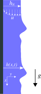
Figure 1: (Color online) Sketch of the profile geometry for a two-dimensional liquid film flowing under the action of gravity down a vertical wall.

Figure 1 shows the problem definition. We consider a thin liquid film flowing under the action of gravity down a vertical planar substrate. The liquid has density $\rho$, kinematic viscosity $\nu$ and surface tension $\sigma$. A Cartesian coordinate system $(x,y)$ is introduced so that $x$ is in the direction parallel to the wall and $y$ is the outward-pointing coordinate normal to the wall. The wall is then located at $y=0$ and the free surface at $y=h(x,t)$. The governing equations are the mass conservation and Navier–Stokes equations along with the no-slip and no-penetration conditions on the wall and the kinematic and tangential and normal stress balance conditions on the free surface.

By introducing a formal parameter $\epsilon$ representing a typical slope of the film, $\epsilon\sim|\partial_{x}h|/h$, we can perform a long-wave expansion of the equations of motion and associated wall and free-surface boundary conditions for $\epsilon\ll 1$. This is based on the observation that because surface tension is generally large, the interfacial waves are typically long compared to the film thickness. This so-called “long-wave approximation” has been central to all thin-film studies (see e.g. Refs. Oron, Davis, and Bankoff, 1997; Kalliadasis and Thiele, 2007) and the small parameter $\epsilon$ is frequently referred to as the “long-wave” or “film parameter”. The long-wave approximation leads to a hierarchy of model equations, starting from a single highly nonlinear partial differential equation for the film thickness $h$, the so-called “Benney equation” Benney (1966) whose region of validity is restricted to near-critical conditions, to equations of the boundary-layer type which are valid away from criticality Chang (1994); Chang and Demekhin (2002); Kalliadasis and Thiele (2007). By neglecting terms of $O(\epsilon^{3})$ and higher, the so-called “second-order boundary-layer equations” read:

$$u_{x}+v_{y} = 0,{}$$ (1a)

$$\mbox{{Re}}(u_{t}+uu_{x}+vu_{y}) = 3(1+\mbox{{W}\!\!{e}}h_{xxx}){}$$ (1b)

$$+u_{yy}-2u_{xx}+[u_{x}|_{h}]_{x},{}$$

$$u|_{0} = v|_{0}=0,{}$$ (1c)

$$u_{y}|_{h} = 4h_{x}(u_{x}|_{h})-v_{x}|_{h},{}$$ (1d)

$$h_{t}+q_{x} = 0,$$ (1e)

where $x$ and $y$ have been non-dimensionalized with the Nusselt flat-film thickness $h_{N}$, the streamwise and cross-stream velocity components, $u$ and $v$, respectively, are both non-dimensionalized by the average Nusselt flat-film velocity, $u_{N}=\mathrm{g}h_{N}^{2}/3\nu$, where $\mathrm{g}$ is the gravitational acceleration, and time $t$ is non-dimensionalized by $h_{N}/u_{N}$. Here, $q=\int_{0}^{h}u\>\mathrm{d}y$ is the streamwise flow rate while the notations $(\cdot)|_{0}$ and $(\cdot)|_{h}$ indicate that the corresponding function is evaluated at $y=0$ and $y=h(x,t)$, respectively. The two dimensionless groups appearing in (1b) are the Reynolds number, measuring the relative importance of inertia to viscous forces and the Weber number, measuring the relative importance of surface tension to gravity, defined as:

$$\mbox{{Re}}=\frac{u_{N}h_{N}}{\nu},\qquad\mbox{{W}\!\!{e}}=\frac{\sigma}{\rho\mathrm{g}h_{N}^{2}}.$$ (2)

We note that elimination of the pressure from the cross-stream momentum equation constitutes the main element of the boundary-layer approximation: by neglecting the inertia terms in this equation, the resulting equation can be integrated across the film to yield the pressure distribution in the film which in turn is substituted into the streamwise momentum equation. It is also important to note that the second-order contributions in the long-wave expansion are given by the two last terms in the right-hand sides of (1b) and (1d) Ruyer-Quil and Manneville (2000). Hence, the second-order boundary layer equations include streamwise viscous-diffusion effects and second-order contributions to the tangential stress at the free surface. These terms play a dispersive role, i.e. they introduce a wavenumber dependence on the speed of the linear waves Ruyer-Quil and Manneville (2002).

By combining the long-wave expansion with a weighted residuals technique based on Galerkin projection in which the velocity field is expanded onto a basis with polynomial test functions, Ruyer-Quil and Manneville Ruyer-Quil and Manneville (1998, 2000, 2002) obtained the following second-order two-field model for the local film thickness and flow rate:

$$\delta q_{t} = \frac{5}{6}h-\frac{5}{2}\frac{q}{h^{2}}+\delta\bigg{(}\frac{9}{7}\frac{q^{2}}{h^{2}}h_{x}-\frac{17}{7}\frac{q}{h}q_{x}\bigg{)}+\frac{5}{6}hh_{xxx}{}$$ (3a)

$$+ \eta\bigg{[}4\frac{q}{h^{2}}(h_{x})^{2}-\frac{9}{2h}q_{x}h_{x}-6\frac{q}{h}h_{xx}+\frac{9}{2}q_{xx}\bigg{]},{}$$

$$h_{t} = -q_{x},$$ (3b)

where lengths, time and velocities in (1) have been rescaled using the following scaling due to Shkadov Shkadov (1977)

$$(x,y) \mapsto (\kappa x,y),{}$$ (4)

$$(u,v) \mapsto (u,\kappa^{-1}v),{}$$ (5)

$$t \mapsto \kappa t,$$ (6)

where $\kappa=\mbox{{W}\!\!{e}}^{1/3}$ and

$$\delta=\frac{3\mbox{{Re}}}{\kappa},\qquad\eta=\frac{1}{\kappa^{2}},$$ (7)

corresponding to a reduced Reynolds and viscous-dispersion number, respectively (note that all second-order/viscous-dispersion terms are gathered in the second line of (3a)). For $\eta=0$ we obtain the first-order model Ruyer-Quil and Manneville (2000), which, much like the second-order one, can be derived from the first-order boundary-layer equations using the long-wave expansion and a weighted residuals technique. It should also be noted that the second-order model contains the same number of parameters as the second-order boundary-layer equations in (1) and hence this model retains the “structure” of these equations (in contrast e.g. with the boundary-layer theory of aerodynamics where the Reynolds number can be scaled away from the boundary layer as the corresponding equations are “simpler” compared to full Navier–Stokes).

This first-order model is similar to the first-order model obtained by Shkadov Shkadov (1967) by combining the long-wave approximation and averaging the basic equations across the fluid layer (effectively, a weighted residual technique with weight function equal to unity) but with different coefficients. As was pointed by Ruyer-Quil and Manneville Ruyer-Quil and Manneville (2000) the second-order model in (3) corrects the shortcomings of the first-order model obtained by Shkadov Shkadov (1967), the principal one being erroneous prediction of the instability onset, i.e. of critical and neutral quantities: (a) it yields a 20$\%$ error of the critical Reynolds number for an inclined film (once again, for a vertical plane the critical Reynolds number vanishes) and (b) the neutral curve (wavenumber for the instability as a function of the Reynolds number) is not in agreement with Orr–Sommerfeld; for this purpose the second-order viscous-dispersion terms are crucial. This is a point that was analyzed carefully by Ruyer-Quil and Manneville Ruyer-Quil and Manneville (1998). These authors contrasted the neutral curve obtained from both the first- and second-order model to the one obtained from the Orr–Sommerfeld eigenvalue problem. The comparison shows clearly that the second-order model is in better agreement with Orr–Sommerfeld than the first-order one.

Finally, it is noteworthy that the parameters $\delta$ and $\eta$ can be expressed as

$$\delta=\Gamma^{-1/3}(3\mbox{{Re}})^{11/9},\qquad\eta=\Gamma^{-2/3}(3\mbox{{Re}})^{4/9},$$ (8)

where $\Gamma=\sigma/(\rho g^{1/3}\nu^{4/3})$ is the Kapitza number that depends on the physical properties of the liquid only. It can then be readily seen that the second-order contributions, controlled by $\eta$, are expected to be more relevant as Re increases and for liquids with either small surface tension or large viscosity.

II.2 Steady-state solutions: solitary pulses

Solitary pulses are traveling-wave solutions propagating at constant speed $c_{0}\equiv c_{0}(\delta,\eta)$, hence stationary in a frame moving with speed $c_{0}$, and sufficiently localized in space. Introducing then in (3) the moving coordinate $x\to x-c_{0}t$ and requiring that waves are stationary in this moving frame, yields:

$$c_{0}q_{0x}-\frac{q_{0}}{7h_{0}}\bigg{(}17q_{0x}-\frac{9q_{0}}{h_{0}}h_{0x}\bigg{)}+\frac{5h_{0}}{6\delta}-\frac{5q_{0}}{2\delta h_{0}^{2}}{}$$

$$+\frac{5h_{0}}{6\delta}h_{0xxx}+\frac{\eta}{\delta}\bigg{[}\frac{4q_{0}}{h_{0}^{2}}(h_{0x})^{2}-\frac{9}{2h_{0}}q_{0x}h_{0x}{}$$

$$-\frac{6q_{0}}{h_{0}}h_{0xx}+\frac{9}{2}q_{0xx}\bigg{]}=0,{}$$ (9a)

$$c_{0}h_{0x}-q_{0x}=0,$$ (9b)

where $q_{0}(x)$ and $h_{0}(x)$ are the stationary solutions for the local flow rate and free-surface shape, respectively. Integrating once (9$b$) yields $q_{0}=c_{0}h_{0}+\alpha$, where $\alpha$ is an integration constant that can be fixed by demanding that the free-surface height approaches the Nusselt flat film solution away from the solitary hump, i.e. $h_{0}=1$ as $x\to\pm\infty$, giving

$$\ q_{0}(x)=c_{0}[h_{0}(x)-1]+\frac{1}{3},$$ (10)

which in turn is used to eliminate $q_{0}$ in (9$a$). The resulting equation is solved numerically with a pseudo-spectral scheme in a periodic domain $[-L,L]$ in which we take the Fast Fourier Transform (FFT) of the equation to obtain a system of nonlinear algebraic equations for the unknown FFT components of $h_{0}$ and the pulse speed $c_{0}$. This system is solved using Newton’s method by choosing an appropriate initial guess.

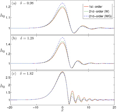
Figure 2: (Color online) Stationary pulse profiles for different values of $\delta$ and two different liquids: water (W) and water+glycerin (WG) for both the first-order ($\eta=0$) and the second-order ($\eta>0$) models.

Figure 2 shows several examples of stationary profiles $h_{0}(x)$. We have used the values $\delta=0.98$, $1.28$, and $1.82$, which correspond to water (W) at $\mbox{{Re}}=3$, $3.75$, and $5$, respectively, and to a water and glycerin 50$\%$ by weight mixture (WG) at $\mbox{{Re}}=1.59$, $2.0$, and $2.66$, respectively (both were used as working fluids in the falling film experiments carried out by Liu et al. Liu, Paul, and Gollub (1993), but for inclined films with small inclination angle). The kinematic viscosities of W and WG are $\nu_{W}=10^{-6}$ m²/s and $\nu_{WG}=5\nu_{W}$, respectively, the densities are $\rho_{W}=1.0$ g/cm³ and $\rho_{WG}=1.13$ g/cm³, respectively, the surface tensions are $\sigma_{W}=69\times 10^{-3}$ N/m and $\sigma_{WG}=72\times 10^{-3}$ N/m, respectively, and the resulting Kapitza numbers are $\Gamma_{W}=3364$ and $\Gamma_{WG}=334$, respectively. It is worth noting that as long as $\delta$ is kept fixed, the first-order model ($\eta=0$) cannot distinguish, for instance, between W at $\mbox{{Re}}=3$ and WG at $\mbox{{Re}}=1.59$. Therefore, the results for the first-order model correspond to both physical situations.

For $\delta=0.98$, $1.28$, and $1.82$, we obtain the following values of the pulse speed and the maximum height, ($c_{0},h_{m}$): ($1.15,1.19$), ($1.34,1.43$), and ($2.44,2.88$), respectively, from the first-order model, and ($1.15,1,20$), ($1.36,1.46$), and ($2.43,2.86$), respectively, from the second-order model using W, and ($1.18,1.23$), ($1.42,1.53$), and ($2.4,2.83$), respectively, from the second-order model using WG. As it has been noticed by Ruyer-Quil and Manneville Ruyer-Quil and Manneville (2000), the differences between the first- and the second-order models as far as solitary pulses are concerned become more significant as $\delta$ is increased. Although the pulse speed and the maximum height do not differ much (differences are appreciable at low values of $\delta$), the capillary ripples that are present downstream of the hump appear to be largely suppressed as a consequence of the second-order viscous-dispersion effects, specially for WG which has higher viscosity.

III Coherent-structure theory for interacting pulses

As it has been emphasized in the Introduction, at sufficiently large distances from the inlet of the film, the dynamics of the free surface is dominated by the presence of localized coherent structures, each of which resembling (infinite-domain) solitary pulses, which continuously interact with each other as quasi particles through attractions and repulsions. The objective of this section is to appropriately extend the recently developed coherent-structure interaction theory for the solitary pulses of the gKS equation Duprat et al. (2009); Tseluiko, Saprykin, and Kalliadasis (2010); Tseluiko et al. (2010) to the two-field model given by (3). This is by far a non-trivial task as we shall demonstrate, e.g. unlike the scalar gKS equation Duprat et al. (2009); Tseluiko, Saprykin, and Kalliadasis (2010); Tseluiko et al. (2010) we now deal with a rather involved vector equation. The aim is to obtain a dynamical system describing the location of each pulse by assuming weak interaction between pulses (i.e. the pulses are sufficiently far from each other and they interact through their tails only). This concept has been applied in many other fields, such as particle physics and quantum mechanics, where one typically deals with a system compound of many particles, and has been used successfully to describe particle–particle interaction. As emphasized in the Introduction, previous coherent-structure theories appear to be either incomplete or some times overlook important details and subtleties, for instance in relation of the spectrum of the operator describing interaction. Moreover, previous coherent-structure theories for film flows in the region of small-to-moderate Reynolds numbers (e.g. Chang, Demekhin, and Kalaidin, 1995; Chang and Demekhin, 2002) were based on the Shkadov model and thus ignored the effect of viscous dispersion.

We start by considering the system of partial differential equations (3) in the frame moving with velocity $c_{0}$ of a single stationary pulse, $x\to x-c_{0}t$. Then we assume that a solution for the local flow rate, $q(x,t)$, and free-surface profile, $h(x,t)$, is given as a superposition of $N$ quasi-stationary pulses located at $x_{1}(t),\,\ldots,\,x_{N}(t)$ (the pulses are labeled from left to right, so that $x_{1}<\cdots<x_{N}$) and a small overlap function, i.e., we postulate the following ansatz:

$$q(x,t) = \frac{1}{3}+\sum_{i=1}^{N}Q_{i}(x,t)+\hat{Q}(x,t),{}$$ (11a)

$$h(x,t) = 1+\sum_{i=1}^{N}H_{i}(x,t)+\hat{H}(x,t),$$ (11b)

where $Q_{i}(x,t)=q_{i}(x,t)-1/3$ and $H_{i}(x,t)=h_{i}(x,t)-1$ and

$$q_{i}(x,t)\equiv q_{0}(x-x_{i}(t))\qquad h_{i}(x,t)\equiv h_{0}(x-x_{i}(t)),$$ (12)

with $q_{0}$ and $h_{0}$ denoting the steady-state solution of (9). A schematic representation of an $N$-pulse solution is given in Fig. 3, where we have defined the distances between two pulses as $\ell_{i}=x_{i+1}-x_{i}$, for $i=1,\,\ldots,\,N-1$. It is worth to mention here that such general formalism derived in the following for the case of $N$ pulses will be ultimately applied to a more simplified system of two pulses only. Next, we consider weak interaction between the pulses by assuming that they are well separated, i.e. $\ell_{i}\gg 1$, so that for each pulse it is enough to consider its interaction with only the immediate neighbours. Because of the exponential decay of functions $H_{0}(x)=h_{0}(x)-1$ and $Q_{0}(x)=q_{0}(x)-1/3$ as $x\rightarrow\pm\infty$, there exist positive constants $C$ and $a$ such that $|H_{0}(x)|\leq C\exp(-a|x|)$ and $|Q_{0}(x)|\leq C\exp(-a|x|)$. We define a small parameter $\varepsilon=\exp{(-a\min_{i}\{\ell_{i}\})}$. Then in the vicinity of each pulse $i$, the tails of the pulses $i-1$ and $i+1$ are $O(\varepsilon)$ and the tails of the remaining pulses are $o(\varepsilon)$. We also assume that the pulse velocities $\dot{x}_{i}(t)$ and the overlap functions $\hat{Q}$ and $\hat{H}$ are $O(\varepsilon)$.

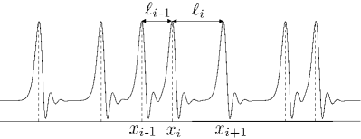
Figure 3: Schematic representation of a solution consisting of a supersposition of $N$ pulses located at $x_{i}$ for $i=1,\,\ldots,\,N$.

By substituting (11) into (3) and expanding up to $O(\varepsilon)$, we obtain a linearized equation in the vicinity of the $i$th pulse for the overlap vector function

$$\hat{\boldsymbol{\Omega}}=\binom{\hat{Q}}{\hat{H}},$$ (13)

that is written as follows:

$$\hat{\boldsymbol{\Omega}}_{t}-\dot{x}_{i}(t){\boldsymbol{\Phi}}_{ix}=\boldsymbol{\mathcal{L}}_{i}\hat{\boldsymbol{\Omega}}+\boldsymbol{\mathcal{J}}_{i}\boldsymbol{\Upsilon}_{i},$$ (14)

where

$${\boldsymbol{\Phi}}_{i}=\binom{q_{i}}{h_{i}},\qquad\boldsymbol{\Upsilon}_{i}=\binom{Q_{i-1}+Q_{i+1}}{H_{i-1}+H_{i+1}},$$ (15)

for $i=1,\,\ldots,\,N$. Note that for $i=1$ and $i=N$, the vector $\boldsymbol{\Upsilon}$ reads as: $\boldsymbol{\Upsilon}_{1}=(Q_{2},H_{2})^{T}$ and $\boldsymbol{\Upsilon}_{N}=(Q_{N-1},H_{N-1})^{T}$. $\boldsymbol{\mathcal{L}}_{i}$ and $\boldsymbol{\mathcal{J}}_{i}$ are the following linear matrix/differential operators:

$$\boldsymbol{\mathcal{L}}_{i}=\begin{pmatrix}\mathcal{L}_{i}^{1}&\mathcal{L}_{i}^{2}\\ \mathcal{L}_{i}^{3}&\mathcal{L}_{i}^{4}\end{pmatrix},\qquad\boldsymbol{\mathcal{J}}_{i}=\begin{pmatrix}\mathcal{J}_{i}^{1}&\mathcal{J}_{i}^{2}\\ 0&0\end{pmatrix},$$ (16)

with the components

$$\mathcal{L}_{i}^{1} = -\frac{5}{2\delta}\frac{1}{h_{i}^{2}}+\frac{18}{7}\frac{q_{i}}{h_{i}^{2}}h_{ix}-\frac{17}{7}\frac{q_{ix}}{h_{i}}+\bigg{(}c_{0}-\frac{17}{7}\frac{q_{i}}{h_{i}}\bigg{)}\partial_{x}{}$$

$$+\frac{\eta}{\delta}\bigg{(}4\frac{h_{ix}^{2}}{h_{i}^{2}}-6\frac{h_{ixx}}{h_{i}}-\frac{9}{2}\frac{h_{ix}}{h_{i}}\partial_{x}+\frac{9}{2}\partial_{xx}\bigg{)},{}$$

$$\mathcal{L}_{i}^{2} = \frac{5}{6\delta}+\frac{5}{\delta}\frac{q_{i}}{h_{i}^{3}}+\frac{17}{7}q_{i}\frac{q_{ix}}{h_{i}^{2}}-\frac{18}{7}q_{i}^{2}\frac{h_{ix}}{h_{i}^{3}}+\frac{5}{6\delta}h_{ixxx}{}$$

$$+\frac{9}{7}\frac{q_{i}^{2}}{h_{i}^{2}}\partial_{x}+\frac{5}{6\delta}h_{i}\partial_{xxx}+\frac{\eta}{\delta}\bigg{[}\frac{9}{2}q_{ix}\frac{h_{ix}}{h_{i}^{2}}-8q_{i}\frac{h_{ix}^{2}}{h_{i}^{3}}{}$$

$$+6q_{i}\frac{h_{ixx}}{h_{i}^{2}}+\bigg{(}8q_{i}\frac{h_{ix}}{h_{i}^{2}}-\frac{9}{2}\frac{q_{ix}}{h_{i}}\bigg{)}\partial_{x}-6\frac{q_{i}}{h_{i}}\partial_{xx}\bigg{]},{}$$

$$\mathcal{L}_{i}^{3} = -\partial_{x},{}$$

$$\mathcal{L}_{i}^{4} = c_{0}\partial_{x},$$

and

$$\mathcal{J}_{i}^{1} = \frac{18q_{i}}{7h_{i}^{2}}H_{ix}-\frac{17}{7h_{i}}(Q_{ix}+Q_{i}\partial_{x}){}$$

$$+\frac{\eta}{\delta}\bigg{(}\frac{4}{h_{i}^{2}}H_{ix}^{2}-\frac{6}{h_{i}}H_{ixx}-\frac{9}{2h_{i}}H_{ix}\partial_{x}\bigg{)},{}$$

$$\mathcal{J}_{i}^{2} = \frac{5}{\delta h_{i}^{4}}(q_{i}H_{i}+Q_{i})+\frac{17q_{i}}{7h_{i}^{2}}Q_{ix}-\frac{18q_{i}^{2}}{7h_{i}^{3}}H_{ix}{}$$

$$+\frac{9q_{i}^{2}-1}{7h_{i}^{2}}\partial_{x}+\frac{5}{6\delta}(H_{ixxx}+H_{i}\partial_{xxx}){}$$

$$+\frac{\eta}{\delta}\bigg{[}\frac{9}{2h_{i}^{2}}Q_{ix}H_{ix}-\frac{8q_{i}}{h_{i}^{3}}H_{ix}^{2}+\frac{6q_{i}}{h_{i}^{2}}H_{ixx}{}$$

$$+\bigg{(}\frac{8q_{i}}{h_{i}^{2}}H_{ix}-\frac{9}{2h_{i}}Q_{ix}\bigg{)}\partial_{x}-\frac{6}{h_{i}}Q_{i}\partial_{xx}\bigg{]}.$$

Equation (14) reveals that the dynamics of the overlap function in the vicinity of the $i$th pulse depends on the spectrum of the linear operator $\boldsymbol{\mathcal{L}}_{i}$ and is influenced by the neighbouring pulses, as indicated by the last term on the right-hand side of (14).

III.1 Analysis of the structure of spectrum of the linearized operator describing interaction

It can be verified numerically that on a periodic domain the operator $\boldsymbol{\mathcal{L}}_{i}$ has a zero eigenvalue with geometric multiplicity one and algebraic multiplicity two (the numerical scheme for constructing the spectrum of $\boldsymbol{\mathcal{L}}_{i}$ will be described shortly). The operator $\boldsymbol{\mathcal{L}}_{i}$ then has a null space spanned by the eigenfunction ${\boldsymbol{\Phi}}_{1}^{i}\equiv{\boldsymbol{\Phi}}_{ix}$ that is associated with the translational invariance of the system. The corresponding generalized zero eigenfunction ${\boldsymbol{\Phi}}_{2}^{i}$ that satisfies $\boldsymbol{\mathcal{L}}_{i}{\boldsymbol{\Phi}}_{2}^{i}={\boldsymbol{\Phi}}_{1}^{i}$ is associated with the Galilean invariance of the system. The aim then is to project the dynamics of the overlap function onto the null space of $\boldsymbol{\mathcal{L}}_{i}$ in the vicinity of the $i$th pulse.

From a physical point of view, the existence of these two dominant modes means that any perturbation to the steady pulse solution will make the pulse to shift (due to the translational mode) and/or to accelerate (due to the Galilean mode). We note that according to the solution ansatz (11), we can assume that the overlap function, $\hat{\boldsymbol{\Omega}}$, is “free of translational modes”. The precise meaning of the latter phrase will be explained later.

Projection onto the null space of the linear matrix/differential operator $\boldsymbol{\mathcal{L}}_{i}$ requires a careful and detailed analysis of its spectrum as well as the spectrum of the adjoint operator $\boldsymbol{\mathcal{L}}_{i}^{*}$ (see Appendix A). The essential spectrum of the operator $\boldsymbol{\mathcal{L}}_{i}$ is given by the dispersion relation of the basic Nusselt state, $(q_{N},h_{N})=(1/3,1)$, in the moving frame. By replacing $(q_{i},h_{i})$ in $\boldsymbol{\mathcal{L}}_{i}$ with the Nusselt state, $\boldsymbol{\mathcal{L}}_{i}$ becomes a matrix operator with constant coefficients and its essential spectrum $\lambda(k)$ satisfies the following equation:

$$\begin{vmatrix}-\frac{5}{2\delta}+\big{(}c_{0}-\frac{17}{21}\big{)}\mathrm{i}k+\frac{9\eta}{2\delta}(\mathrm{i}k)^{2}-\lambda&\frac{5}{2\delta}+\frac{1}{7}\mathrm{i}k+\frac{5}{6\delta}(\mathrm{i}k)^{3}-\frac{2\eta}{\delta}(\mathrm{i}k)^{2}\\ &\\ -\mathrm{i}k&c_{0}\mathrm{i}k-\lambda\end{vmatrix}=0$$ (17)

for $k\in\mathbb{R}$. The locus of the essential spectrum is shown as a solid line in Fig. 4, and coincides with the locus of the essential spectrum of the adjoint operator (see Appendix A), as expected. We note that part of the essential spectrum is unstable. As it has been demonstrated in previous studies (e.g. Refs. Chang, Demekhin, and Kalaidin, 1995; Tseluiko, Saprykin, and Kalliadasis, 2010; Tseluiko et al., 2010), the unstable part of the essential spectrum is connected with the flat film instability and can be excluded from our consideration.

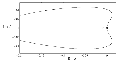
Figure 4: Spectrum of $\boldsymbol{\mathcal{L}}_{i}$ for $\delta=0.98$ for the second-order model with the physical parameters corresponding to W. The solid line represents the essential spectrum and the crosses represent the point spectrum.

To analyze numerically the spectrum of $\boldsymbol{\mathcal{L}}_{i}$, we first compute the solution for $h_{i}$ and $q_{i}$ on a finite $2L$-periodic interval by using a pseudo-spectral method. The matrix representation of the linear operator is obtained by applying each component of $\boldsymbol{\mathcal{L}}_{i}$ to a plane wave, i.e. $\mathcal{L}_{i}^{j}\rightarrow\mathcal{L}_{i}^{j}\mathrm{e}^{\mathrm{i}k_{n}x}$, for $j=1,\,\ldots,\,4$, and transforming to Fourier space the resulting functions. By computing this operation $\forall k_{n}=n\pi/L$ of the truncated Fourier series of $h_{i}$, we are able to get the $n$th column of the Fourier matrix representation of $\mathcal{L}_{i}^{j}$. We then analyze the eigenvalues and eigenvectors for the resulting matrix. Our results show that, in addition to the essential spectrum and the zero eigenvalue, which is embedded into the essential spectrum, there is one more eigenvalue, which is negative and isolated. The eigenvalues are depicted as crosses in Fig. 4. In Fig. 5 we depict the two components of the generalized eigenfunction ${\boldsymbol{\Phi}}_{2}^{i}$ given by the solution of $\boldsymbol{\mathcal{L}}_{i}{\boldsymbol{\Phi}}_{2}^{i}={\boldsymbol{\Phi}}_{1}^{i}$ and corresponds to the Galilean mode.

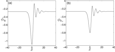
Figure 5: Components of the generalized zero eigenfunction ${\boldsymbol{\Phi}}_{2}^{i}=(\phi_{q_{i}},\phi_{h_{i}})$ corresponding to the Galilean mode.

On a periodic domain, the discrete part of the adjoint operator also coincides with the discrete part of $\boldsymbol{\mathcal{L}}_{i}$ (see Appendix A). We find that the eigenfunction corresponding to the zero eigenvalue on a periodic domain is merely a constant

$${\boldsymbol{\Psi}}_{1}^{i}=\binom{0}{m},$$ (18)

and the generalized zero eigenfunction ${\boldsymbol{\Psi}}_{2}^{i}=(\psi_{q_{i}},\psi_{h_{i}})^{T}$ has to be found numerically. Its components are shown in Fig. 6 for different values of the periodicity interval.

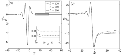
Figure 6: Components of the generalized adjoint eigenfunction ${\boldsymbol{\Psi}}_{2}^{i}=(\psi_{q_{i}},\psi_{h_{i}})$ for different values of the period $L$.

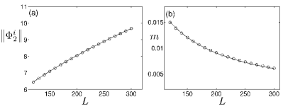
Figure 7: (a) Norm of the generalized zero eigenfunction of $\boldsymbol{\mathcal{L}}_{i}$, for different values of the system size $L$. The solid line corresponds to a function proportional to $L^{1/2}$. (b) Constant value $m$ of the zero eigenfunction of $\boldsymbol{\mathcal{L}}_{i}^{*}$ for different $L$. The solid line corresponds to a function proportional to $1/L$.

In our analysis, we have normalized the eigenfunctions so that the following conditions hold:

$$\langle{\boldsymbol{\Phi}}_{1}^{i},{\boldsymbol{\Psi}}_{1}^{i}\rangle=0,\qquad\langle{\boldsymbol{\Phi}}_{1}^{i},{\boldsymbol{\Psi}}_{2}^{i}\rangle=1,{}$$

$$\langle{\boldsymbol{\Phi}}_{2}^{i},{\boldsymbol{\Psi}}_{1}^{i}\rangle=1,\qquad\langle{\boldsymbol{\Phi}}_{2}^{i},{\boldsymbol{\Psi}}_{2}^{i}\rangle=0,$$

where $\langle\cdot,\cdot\rangle$ denotes the inner product in $L_{\mathbb{C}}^{2}(-L,L)$.

We now examine the behavior of the eigenfunctions in the limit $L\to\infty$. First, we note that both components $\phi_{q_{i}}$ and $\phi_{h_{i}}$ corresponding to the Galilean mode ${\boldsymbol{\Phi}}_{2}^{i}$ do not decay to zero at infinities $x\to\pm\infty$ (cf. Fig. 5), and therefore we have that $|\!|{\boldsymbol{\Phi}}_{2}^{i}|\!|\equiv\sqrt{\langle{\boldsymbol{\Phi}}_{2}^{i},{\boldsymbol{\Phi}}_{2}^{i}\rangle}\to\infty$ as the system size is increased, see Fig. 7(a). This means that on an infinite domain the zero eigenvalue has both algebraic and geometric multiplicity equal to unity and the null space of $\boldsymbol{\mathcal{L}}_{i}$ is spanned only by the translational mode. Second, we also note that the constant $m$ in (18) corresponding to the zero eigenfunction of $\boldsymbol{\mathcal{L}}_{i}^{*}$ tends to zero as the system size is increased (see Fig. 7(b)), meaning that $\boldsymbol{\mathcal{L}}_{i}^{*}{\boldsymbol{\Psi}}_{2}^{i}\to 0$ as $L\to\infty$, and thus, we have that the function ${\boldsymbol{\Psi}}_{2}^{i}$ belongs to the null space of $\boldsymbol{\mathcal{L}}_{i}^{*}$. As it is shown in Fig. 6, the component $\psi_{q_{i}}$ decays to zero at infinities for $L\to\infty$, and the component $\psi_{h_{i}}$ tends to different constants as $x\to\pm\infty$, and therefore $|\!|{\boldsymbol{\Psi}}_{2}^{i}|\!|\to\infty$.

We then conclude that the zero eigenvalue of $\boldsymbol{\mathcal{L}}_{i}$ is not isolated but belongs to the essential spectrum (and has both algebraic and geometric multiplicity equal to unity on an infinite domain with the null space of $\boldsymbol{\mathcal{L}}_{i}$ spanned by the translational mode ${\boldsymbol{\Phi}}_{1}^{i}$). Also, zero is not in the point spectrum of the adjoint operator, $\boldsymbol{\mathcal{L}}_{i}^{*}$ on an infinite domain (its null space is spanned by a constant and a vector function, one component of which does not decay to zero at infinities). These two points complicate the formal projections of the overlap function onto the translational mode (the null space of $\boldsymbol{\mathcal{L}}_{i}$).

We remark here that we find similar spectrum features between the second-order model and the gKS equation Duprat et al. (2009); Tseluiko, Saprykin, and Kalliadasis (2010); Tseluiko et al. (2010). We first note that although the Galilean mode ${\boldsymbol{\Phi}}_{2}^{i}$ in the gKS equation is given by a constant, it is observed in both models that its norm tends to infinity as $L$ is increased, and therefore it can be excluded from the projections on the translational mode. In addition, we find the same behaviour of the $h$-component of the generalized eigenfunction of the adjoint operator (cf. Fig. 6$b$) and the generalized eigenfunction of the interaction problem with the gKS equation, namely a jump at infinity in both cases and, therefore, an infinite norm for the corresponding eigenfunction. As was pointed out in the coherent-structure theory for the gKS prototype Tseluiko et al. (2010), it is possible to overcome such difficulties by making use of a formal procedure in a weighted space of functions that decay exponentially at $+\infty$. We shall therefore apply such a formalism in the present study.

III.2 Formulation in a weighted functional space

Projections onto the null space can be made rigorous by choosing an appropriate weighted space. Following the formulation used in Ref. Pego and Weinstein, 1994 for the Korteweg–de Vries equation and in Refs. Tseluiko, Saprykin, and Kalliadasis, 2010; Tseluiko et al., 2010 for the gKS equation, we shall restrict our projections to the following weighted space:

$$L_{a}^{2}=\{{\boldsymbol{u}}:\,\mathrm{e}^{ax}{\boldsymbol{u}}\in L_{\mathbb{C}}^{2}\},$$ (19)

with the inner product $\langle\boldsymbol{u},\boldsymbol{v}\rangle_{a}=\langle\mathrm{e}^{ax}\boldsymbol{u},\mathrm{e}^{ax}\boldsymbol{v}\rangle$, and $a>0$. The spectrum of the matrix/differential operator $\boldsymbol{\mathcal{L}}_{i}$ in $L_{a}^{2}$ can be studied there through the matrix/differential operator defined by

$$\boldsymbol{\mathcal{L}}_{i}^{a}\boldsymbol{u}=\mathrm{e}^{ax}\boldsymbol{\mathcal{L}}_{i}(\mathrm{e}^{-ax}\boldsymbol{u}),$$ (20)

on $L_{\mathbb{C}}^{2}$. More precisely, one can easily see that the essential spectrum $\lambda_{a}(k)$ of $\boldsymbol{\mathcal{L}}_{i}^{a}$ is then given by (17) by replacing $\mathrm{i}k$ with $\mathrm{i}k-a$. The interesting point of working in such a weighted space is that for certain values of $a$, it is possible to completely shift the essential spectrum to the left in the complex plane (see Fig. 8), and therefore, the pulses may become spectrally stable by choosing an appropriate value of $a$. Such a shift of the essential spectrum means that the pulses are transiently unstable but not absolutely unstable, i.e. any localized disturbance is convected to $-\infty$ in a frame moving with the velocity of the pulse Sandstede and Scheel (2000). [The essential part of the spectrum typically leads to an expanding and growing radiation wave packet such that its left end travels upstream and right end downstream (absolute instability). If the speed of the right end of the wave packet is larger than that of a solitary pulse, the pulse is destroyed, i.e. it is “absolutely unstable”].

It is this absolute instability of the pulses which is responsible for the complex turbulent-like spatio-temporal chaos observed in the KS equation, i.e. disordered dynamics in both time and space and without clearly identifiable soliton-like coherent structures. For the gKS equation Tseluiko, Saprykin, and Kalliadasis (2010); Tseluiko et al. (2010) there exists a critical value of the parameter controlling dispersion (the coefficient multiplying the third-derivative term in the equation), below which it is no longer possible to shift the spectrum to the left half-plane and the behavior of the gKS equation is spatio-temporal chaos like with the KS one. In our case, however, for all $\delta$ values (or, equivalently, the Reynolds number) we examined (up to 12) it is always possible to shift the spectrum completely to the left half of the complex plane, implying that dispersion effects prevent the system from evolving into spatio-temporal chaos.

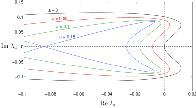
Figure 8: (Color online) Essential spectrum of $\boldsymbol{\mathcal{L}}_{i}^{a}$ for $\delta=0.98$ with physical parameters for W and different values of $a$.

From the numerical point of view, having a stable essential spectrum means that the instabilities due to numerical noise could be eliminated and the temporal evolution of solitary waves could be obtained for sufficiently long times. In order to have then a stable essential spectrum, we substitute

$$q=\mathrm{e}^{-ax}g+1/3,\qquad\qquad h=\mathrm{e}^{-ax}f+1$$ (21)

into (3) to obtain the following equations for $g$ and $f$:

$$g_{t} = c_{0}(g_{x}-ag)+\frac{5}{6\delta}f-\frac{5}{2\delta}\frac{g-(1/3)\mathrm{e}^{-ax}f^{2}-(2/3)f}{h^{2}}{}$$ (22a)

$$-\frac{17}{7}\frac{q}{h}(g_{x}-ag)+\frac{9}{7}\frac{q^{2}}{h^{2}}(f_{x}-af)+\frac{5}{6\delta}h(f_{xxx}{}$$

$$-3af_{xx}+3a^{2}f_{x}-a^{3}f)+\frac{\eta}{\delta}\bigg{[}4\frac{q}{h^{2}}\mathrm{e}^{-ax}(f_{x}-af)^{2}{}$$

$$-\frac{9}{2}\frac{\mathrm{e}^{-ax}}{h}(g_{x}-ag)(f_{x}-af)-6\frac{q}{h}(f_{xx}{}$$

$$-2af_{x}+a^{2}f)+\frac{9}{2}(g_{xx}-2ag_{x}+a^{2}g)\bigg{]},{}$$

$$f_{t} = c_{0}(f_{x}-af)-(g_{x}-ag).$$ (22b)

Integrating numerically the above equations with an appropriate value of $a$, ensures that the flat-film instability will not be excited and the dynamics of the pulses will not be affected by any numerical noise. This will be particularly useful, for instance, when studying the interaction between two pulses, see Sec. IV.1.

The other important consequence of working in a weighted space is that the projections onto the null space can now be made properly, since the zero eigenvalue becomes isolated. We note that the null space of $\boldsymbol{\mathcal{L}}_{i}^{a}$ is only spanned by the zero eigenfunction, ${\boldsymbol{\Phi}}_{a}^{i}=\mathrm{e}^{ax}{\boldsymbol{\Phi}}_{1}^{i}$. Also, the zero eigenfunction of the adjoint operator, defined by $\boldsymbol{\mathcal{L}}_{i}^{a*}=\mathrm{e}^{-ax}\boldsymbol{\mathcal{L}}_{i}^{*}(\mathrm{e}^{ax}f)$, can be written as

$${\boldsymbol{\Psi}}_{a}^{i}=\mathrm{e}^{-ax}({\boldsymbol{\Psi}}_{2}^{i}-\lim_{x\to-\infty}{\boldsymbol{\Psi}}_{2}^{i})$$

which now has a finite norm. Therefore, we will use the projection operator

$$P_{i}(\boldsymbol{f})=\langle\boldsymbol{f},{\boldsymbol{\Psi}}_{a}^{i}\rangle_{a}{\boldsymbol{\Phi}}_{a}^{i},$$ (23)

for projecting onto the the null space of $\boldsymbol{\mathcal{L}}_{i}^{a}$.

III.3 Pulse interactions and bound-state formations

By applying the projection operator $P_{i}$ to (14) rewritten in an exponentially weighted space and assuming that the overlap function is “free of translational modes” meaning that it is in the null spaces of the projections, i.e. $P_{i}(\mathrm{e}^{ax}\hat{\boldsymbol{\Omega}})=0$, we obtain the following dynamical system for the pulse locations:

$$\dot{x}_{i}(t)=\int_{-\infty}^{\infty}\!\!\!\big{[}(H_{i-1}+H_{i+1})(c_{0}\mathcal{J}_{i}^{1*}+\mathcal{J}_{i}^{2*})\psi_{q_{i}}\big{]}\,\mathrm{d}x,$$ (24)

for $i=2,\,\ldots,\,N-1$, and

$$\dot{x}_{1}(t)=\int_{-\infty}^{\infty}\!\!\!\big{[}H_{2}(c_{0}\mathcal{J}_{1}^{1*}+\mathcal{J}_{1}^{2*})\psi_{q_{1}}\big{]}\,\mathrm{d}x,{}$$ (25)

$$\dot{x}_{N}(t)=\int_{-\infty}^{\infty}\!\!\!\big{[}H_{N-1}(c_{0}\mathcal{J}_{N}^{1*}+\mathcal{J}_{N}^{2*})\psi_{q_{N}}\big{]}\,\mathrm{d}x,$$ (26)

where $\mathcal{J}_{i}^{1*}$ and $\mathcal{J}_{i}^{2*}$ correspond to the adjoint operator components of the matrix/differential operator $\boldsymbol{\mathcal{J}}_{i}$ (see Appendix A), and $\psi_{q_{i}}$ is the first component of the adjoint eigenfunction ${\boldsymbol{\Psi}}_{2}^{i}$. Here we have also made use of the relation $Q_{i}=c_{0}H_{i}$. If we define the function $\overline{\psi}_{i}\equiv(c_{0}\mathcal{J}_{i}^{1*}+\mathcal{J}_{i}^{2*})\psi_{q_{i}}$, and use the notations

$$S_{1}(\ell)\equiv\int_{-\infty}^{\infty}\!\!H_{0}(x-\ell/2)\overline{\psi}_{0}(x+\ell/2)\mathrm{d}x,{}$$ (27)

$$S_{2}(\ell)\equiv\int_{-\infty}^{\infty}\!\!H_{0}(x+\ell/2)\overline{\psi}_{0}(x-\ell/2)\mathrm{d}x,$$ (28)

where $H_{0}(x)=h_{0}(x)-1$ and $\overline{\psi}_{0}$ is such that $\overline{\psi}_{i}(x)=\overline{\psi}_{0}(x-x_{i})$, (24) can be finally rewritten as

$$\dot{x}_{i}(t)=S_{1}(x_{i+1}-x_{i})+S_{2}(x_{i}-x_{i-1}),$$ (29a)

for $$i=2,...,N-1 i=1 i=N$$. For and , we have

$$\dot{x}_{1}(t)=S_{1}(x_{2}-x_{1})$$ (29b)

and

$$\dot{x}_{N}(t)=S_{2}(x_{N}-x_{N-1}),$$ (29c)

respectively. Therefore, the time-evolution of the $i$th pulse location is controlled on the one hand by the function $S_{1}(x)$, which describes the interaction with the monotonic tail of the downstream pulse $i+1$, and on the other hand, by the function $S_{2}(x)$ that describes the interaction with the oscillatory capillary ripples of the upstream pulse $i-1$.

Let us consider the case of only two pulses interacting with each other, i.e. a binary interaction scenario. From Eq. (29a), we can write an equation for the separation distance between the pulses, $\ell(t)=x_{2}(t)-x_{1}(t)$, as:

$$\dot{\ell}(t)=S_{2}(\ell)-S_{1}(\ell).$$ (30)

The fixed points of the above equation are given by

$$S_{1}(\ell_{n})=S_{2}(\ell_{n}),$$ (31)

which predicts the different distances $\ell_{n}$ at which both pulses travel at the same velocity, giving rise then to the formation of bound states. Figure 9 shows the graphs of $S_{1}$ and $S_{2}$ for two different values of $\delta$ for the second-order model using W. Interestingly, since $S_{1}(\ell)$ and $S_{2}(\ell)$ represent the velocity of the pulses located at $x_{1}$ and $x_{2}$, respectively, we can also predict both the velocity of the bound state relative to $c_{0}$, i.e. $c_{n}=S_{1}(\ell_{n})$, and its stability. Stable and unstable bound states are represented by solid circles and crosses, respectively in Fig. 9. As long as $S_{2}>S_{1}$, we have that $\dot{x}_{2}>\dot{x}_{1}$ so that the second pulse moves faster than the first one leading to an increase of $\ell$, and therefore, both pulses repel each other. On the other hand, when $S_{2}<S_{1}$, the first pulse is moving faster than the second one leading to a decrease of $\ell$, and therefore both pulses attract each other.

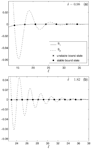
Figure 9: Functions $S_{1}$ and $S_{2}$ (solid and dashed lines, respectively) for (a) $\delta=0.98$ and (b) $\delta=1.82$. The black circles and crosses correspond to stable and unstable bound-state separation distances, respectively.

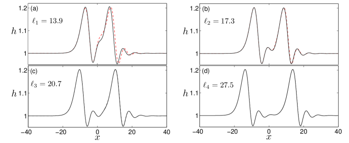
Figure 10: (Color online) Numerically computed bound states (dashed lines) compared to the theoretical predictions (solid lines) given by (32). The physical parameters correspond to W with $\delta=0.98$.

From a physical point of view, such oscillatory behavior of attractions and repulsions between pulses can be understood in terms of the interaction between the periodic capillary waves ahead of the first pulse and the monotonic tail behind the second pulse (see Duprat et al., 2009). More precisely, the oscillatory shape of the free surface ahead of the hump induces a sign change of the capillary pressure difference across the free surface, $\Delta p_{c}\sim\sigma h_{xx}$. Let us consider the interaction of pulse 1 and pulse 2, which are located at $x_{1}$ and $x_{2}$, respectively. Note that according to our labeling, $x_{1}<x_{2}$, i.e. pulse 1 is located to the left of pulse 2. When the tail of pulse 2 overlaps with a maximum of one of the capillary waves of pulse 1, there is a drainage process of liquid from the oscillatory tail of pulse 1 to pulse 2 due to the positive pressure difference across the free surface at the overlaping area between both pulses. This, in turn, generates an increase of both the height and the speed of pulse 2, on the one hand, and a decrease of the height and the speed of pulse 1, on the other hand. As a result, the distance between the pulses increases corresponding to repulsion. The opposite behavior occurs when the tail of pulse 2 overlaps with a minimum of one of the capillary waves of pulse 1, giving rise then to an attraction process. When the frequency and the amplitude of the capillary oscillations are increased by increasing $\delta$, the number of bound states observed in a given interval by such attraction/repulsion mechanism increases accordingly [see Fig. 9(b)], as expected. Note, however, that we are always assuming that the pulses are well-separated, and although the theory predicts bound-state formation at relatively short distances, these are not expected to be observed.

IV Numerical results

In this section we present extensive numerical experiments for the second-order model (3). More specifically, we investigate numerically the temporal evolution of a superposition of two pulses as an initial condition and resulting attractive and repulsive dynamics giving rise to formation of bound states. We compare the numerical results with the coherent-structure theory developed in the previous section. By imposing a localized random initial condition, we are able to study how several pulses interact with each other to self-organize and form bound states compound of two or more pulses. The effect of viscous dispersion on the bound-state formation will be elucidated by systematically integrating both the first- and second-order models for the physical parameters corresponding to W and WG.

IV.1 Superposition of two pulses

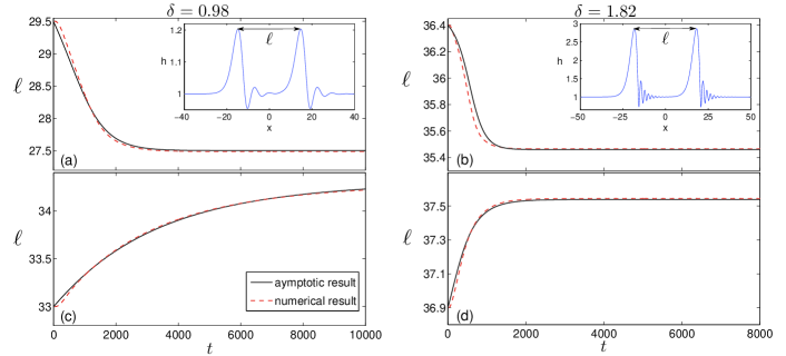
Figure 11: (Color online) Evolution of the separation distance between two pulses for $\delta=0.98$ and $\delta=1.82$. The initial separation distances are $\ell_{0}=29.5$ (a) and $33$ (c) for $\delta=0.98$, and $\ell_{0}=36.4$ (b) and $33.9$ (d) for $\delta=1.82$. Solid lines correspond to the numerical solution of the theoretical model given by (30), and dashed lines are the numerical solution of the second-order model in a weighted space, (22), with $a=0.1$.

Two-pulse bound states can be constructed numerically by solving (9) with an initial guess consisting of a superposition of two pulses separated by the theoretically predicted distance. We use the numerical method of Sec. II.2, based on a combination of a pseudo-spectral method and Newton’s method, and the numerical result is compared to the superposition of two pulses,

$$h=1+H_{0}(x+\ell_{n}/2)+H_{0}(x-\ell_{n}/2),$$ (32)

where $\ell_{n}$ corresponds to the distances obtained by (31). Figure 10 shows the results in the case of $\delta=0.98$ for the bound states predicted at $\ell_{1}\approx 13.9$, $\ell_{2}\approx 17.3$, $\ell_{3}\approx 20.7$, and $\ell_{4}\approx 27.5$ [cf. Fig. 9(a)]. As expected, the longer separation distance between the pulses is, the better the agreement between the theory and the numerical solution becomes. In particular, at $\ell_{3}\approx 20.7$ and $\ell_{4}\approx 27.5$, the numerical solution and the superposition of two pulses with the theoretically predicted bound-state separation distance are practically indistinguishable. It is interesting to note that the numerical scheme only converged when the pulse separation distance for the initial guess was sufficiently close to the value predicted by the theory. We also find good agreement between the bound-state velocities relative to $c_{0}$ predicted theoretically and found numerically: the numerical values are $c_{1}\approx-0.00302$, $c_{2}\approx-0.00039$, and $c_{3}\approx-0.00006$, which are to be compared with the theoretical predictions of $-0.00197$, $-0.00035$, and $-0.00006$, respectively.

To check the attraction/repulsion dynamics between two pulses predicted by the theory, we study numerically the time-evolution of two pulses separated by an initial distance $\ell_{0}$ which is close to either a stable or unstable bound-state separation distance. We numerically integrate both the second-order model (22) in a weighted space, and the theoretical model given by (30). As it has been emphasized in Sec. III.2, working in the weighted space $L_{a}^{2}$ has the advantage of the essential spectrum being shifted to the left half of the complex plane. Hence, any instability on the flat film region that originates from numerical noise is eliminated, which then allows us to follow the temporal evolution of the two pulses for sufficiently long times. Equations (22) are integrated by choosing $a=0.1$. To solve (22) numerically we use the FFT to obtain the Fourier and the inverse Fourier transforms of $g$ and $f$ in the right-hand sides of (22) and a fourth-order Runge–Kutta method to march forward in time. A typical time step is $\Delta t=0.0025$ and the periodic domain $[-L,L]$, with $L=120$, is discretized into 2000 intervals.

The results for $\delta=0.98$ and $1.82$ for W are presented in Fig. 11. The interaction between the two pulses is attractive when the pulses are initially separated by $\ell_{0}=29.5$ and $36.4$ for $\delta=0.98$ and $1.82$, respectively, converging to the predicted stable bound states with the separation distances approximately $27.5$ and $35.3$, respectively. Likewise, the dynamics is repulsive when the pulses are initially separated by $\ell_{0}=33$ and $36.9$ for $\delta=0.98$ and $1.82$, respectively. The separation distances then converge to the predicted stable bound-state separation distances $34.3$ and $37.5$, respectively. In all cases, we found a very good agreement between the theory and the numerical results.

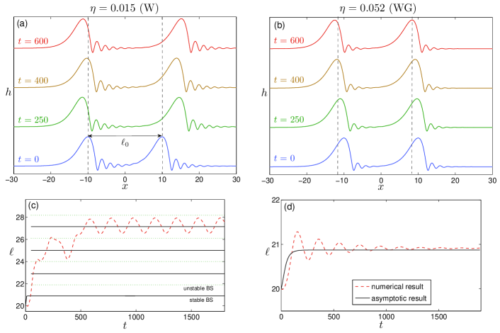
Figure 12: (Color online) Oscillatory interaction between two pulses observed at $\delta=1.82$ in the second-order model by using the physical parameters of W [(a), (c)] and WG [(b), (d)]. The top panels show the two-pulse system profile at four different times: $t=0$, $250$, $400$, and $600$, from bottom to top, respectively. The bottom panels show the comparison between the numerical result obtained by integrating the second-order model in a weighted space, given by equations (22) with $a=0.1$ (red dashed line) and the asymptotic result predicted by the theoretical model (30). The solid and dotted lines in (c) represent the stable and unstable bound states (BS), respectively, predicted by the theory. The pulses seem lock on at certain average distances close to those predicted by the weak interaction theory.

Interestingly, a different interaction behaviour emerges as both pulses are placed close enough to each other so that the assumption of a well-separated distance between them is not valid anymore and the interaction is no longer weak. Figures 12($a$) and 12($c$) depicts the temporal evolution of two pulses separated by an initial distance $\ell_{0}=20$ for a relatively high Reynolds number ($\delta=1.82$) in the second-order model using the physical parameters for W (which gives a value of $\eta=0.015$ for the viscous-dispersion number). We observe that both pulses attract and repel each other in an oscillatory manner, giving rise to a rapid fluctuating growth of the initial separation length until they reach an oscillatory steady-state of constant frequency and amplitude [the dashed line in Fig. 12($c$)]. Is is remarkable that although such an oscillatory dynamics cannot be captured by our weak-interaction theory, the final separation length around both pulses are oscillating corresponds to a stable bound state predicted by the theory (solid lines), and the amplitude of the oscillations is delimited within the distance between two consecutive unstable bound states (dotted lines). This type of oscillatory interaction between two pulses was first observed by Malamataris et al. Malamataris, Vlachogiannis, and Bontozoglou (2002) in direct numerical simulations of the full Navier–Stokes equations with wall and free-surface boundary conditions, and was attributed to the competition of the strong fluctuations on the capillary pressure at the overlapping area between the pulses, and the nonlinear response of the solitary hump when it is perturbed from its stationary shape. In this sense, if we consider stronger viscous dispersion effects, leading to smaller amplitude of the capillary fluctuations in the front tail of the pulse (cf. Fig. 2), such oscillatory interaction can be largely or completely removed. Indeed, Fig. 12($b$) repeats the same numerical experiment but taking the physical parameters corresponding to WG, which is more viscous than water and thus gives the value of $\eta=0.052$ for the viscous dispersion number. We observe that such oscillatory interaction is largely reduced and the two pulses eventually reach a stable bound state in agreement with our weak-interaction theory. This is a clear manifestation of the fact that including the second-order viscous-dispersion effects, ignored in all previous film-flow interaction studies, can be crucial to obtaining an accurate description of the interaction between pulses.

IV.2 Localized random initial condition

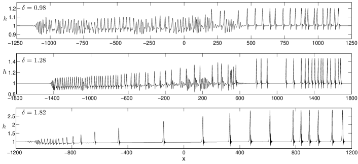
Figure 13: Typical numerical solutions of the second-order model (3) in extended domains for $\delta=0.98,\,1.28$, and $1.82$ at $t=2250,\,1700$, and $450$, respectively (panels (a), (b), and (c), respectively). See supplementary material at [URL will be inserted by AIP] for the time evolution of a localised random initial condition for $\delta=0.98$ in the frame moving with velocity $c_{0}$.

We also integrate (3) by considering both the first- ($\eta=0$) and second-order model ($\eta>0$), and imposing a localized random initial condition. In our simulations, we have used the parameter values for both W and WG. To obtain an appropriate random representation of a differentiable function but with a sufficiently high frequency content we construct the initial condition by using the following random function:

$$h_{\mathrm{in}}(x)=\frac{\gamma_{0}}{\sqrt{N}}\sum_{m=1}^{N}\bigg{(}\alpha_{m}\sin\frac{k_{0}m}{N}x+\beta_{m}\cos\frac{k_{0}m}{N}x\bigg{)},$$ (33)

which has been recently proposed in Ref. Savva, Kalliadasis, and Pavliotis, 2010 in the context of wetting of disordered substrates. Here, $\gamma_{0}$ and $k_{0}$ are the characteristic amplitude and wavenumber, respectively, $N$ is a large positive integer, and $\alpha_{m}$ and $\beta_{m}$ are statistically independent normal variables with zero mean and unit variance. It can be shown that in the limit of $\gamma_{0}k_{0}\ll 1$ and $N\to\infty$, $h_{\mathrm{in}}(x)$ is a band-limited white noise. To get a localized perturbation, $h_{\mathrm{in}}(x)$ is then multiplied by the function $\theta(x)=[\tanh(x)-\tanh(x+L_{c})]/2$, where $L_{c}$ is the length of the disturbance. In our simulations we have chosen $\gamma_{0}=0.05$, $k_{0}=1$, $N=2000$, and $L_{c}=500$.

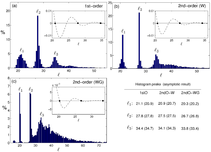
Figure 14: (Color online) Histograms of the pulse-separation distances for $\delta=0.98$ in (a) the first-order model ($\eta=0$), (b) the second-order model with the parameter values corresponding to W ($\eta=0.011$), and (c) the second-order model with the parameter values corresponding to WG ($\eta=0.041$). The table shows the locations of the peaks observed in the histograms obtained for the 1st-order (1stO) and 2nd-order (2ndO) models compared to the values predicted by (29a), plotted in the insets of each panel, where the dashed and solid lines correspond to the $S_{2}$ and $S_{1}$ functions, respectively.

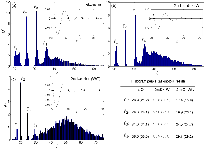
Figure 15: (Color online) Histograms of the pulse-separation distances for $\delta=1.28$ in (a) the first-order model ($\eta=0$), (b) the second-order model with the parameter values corresponding to W ($\eta=0.013$), and (c) the second-order model with the parameter values corresponding to WG ($\eta=0.046$). The table shows the locations of the peaks observed in the histograms compared to the values predicted by the model given by (29a), plotted in the insets of each panel, where the dashed and solid lines corresponds to the $S_{2}$ and $S_{1}$ functions, respectively.

To accelerate the computational efficiency of our numerical scheme, we have used a Runge–Kutta–Fehlberg method with dynamic time-step adjustment. At each time step this scheme computes two different solutions and compares them. The time-step is the redefined according to the agreement between both solutions. We impose a minimum time step $\Delta t=0.001$ (that is reached only in computations for large values of $\delta$), and we are able to use time steps as large as $\Delta t=0.01$. We integrated equations (3) on a periodic domain $[-L,L]$ discretized into $2M$ intervals by using the FFT to obtain the Fourier and the inverse Fourier transforms of $q$ and $h$ in the right-hand sides of (3). Note that the use of periodic boundary conditions turns out to be quite convenient to solve unforced systems in the frame moving with velocity $c_{0}$. We used the following values: $L=1250$, $1800$, and $1200$ and $M=2000$, $3000$, and $4000$ for $\delta=0.98$, $1.28$, and $1.82$, respectively. The initial disturbance results in an expanding wave packet whose left envelope travels upstream (absolute instability; see our comment in Sec. III.2) and the right one travels with a velocity lower to that of an individual pulse. The wave packet grows as it propagates and gives birth to a number of pulses escaping the expanding wave packet. The equations were integrated up to $t=2250$, $1700$, and $450$ for $\delta=0.98$, $1.28$, and $1.82$, respectively. Beyond these times the rear side of the expanding packet starts to interact with the front pulses. Figure 13 shows typical solutions for the different values of $\delta$ by using the physical parameters of W in the second-order model. In order to compute the histograms of the pulse-separation distances for $\delta=0.98$ and $1.28$, we took into account the first 12 pulses which are located at the righmost part of the corresponding panels of Fig. 13, and performed 600 different realisations, giving a total number of 6600 separation lengths. For $\delta=1.82$, we took into account the first 6 pulses, and performed 1200 realisations, giving 6000 separation lengths in total.

Figure 14 depicts the results obtained for the first- and second-order models at $\delta=0.98$ for W and WG at $\mbox{{Re}}=3$ and $1.59$, respectively. Panel (a) shows the histogram of the separation distances between pulses obtained from the first-order model and panels (b) and (c) from the second-order model for W and WG, respectively. The inset in each panel shows the corresponding $S_{1}$ and $S_{2}$ functions from the theoretical model given by (30). We first note that in all the cases the distributions for the pulse separation distances are mainly characterized by three peaks that correspond in each case to the theoretically predicted distances at which two-pulses bound states are formed (see table in Fig. 14). It is interesting to note that the peaks appear to be broad, indicating that dynamic interaction between pulses seems to persist indefinitely. Such interaction, however, is affected by viscous dispersion, obtaining that the peaks of the distributions become more pronounced and sharper for the simulations of the second-order model, specially the ones observed at short distances, $\ell_{1}$ and $\ell_{2}$ [cf. 14(b) and 14(c)]. Also, while the locations at which bound-states are formed are approximately the same in all cases, the dominant peaks in the distribution change as the viscous-dispersion effects are increased. In particular, we observe that the distribution for the first-order simulations is mainly dominated by the bound states formed at $\ell_{2}$, whereas the distributions for the second-order simulations are dominated by the peaks at $\ell_{1}$ and $\ell_{2}$, particularly in the WG case where both peaks have approximately the same probabilities. We also note a small peak, less than $0.5\%$, in the second-order WG results, reflecting that the shortest pulse-separation distance can be affected by second-order terms. A more clear picture on the effect of viscous dispersion on pulse dynamics is expected to emerge as $\delta$ is increased.

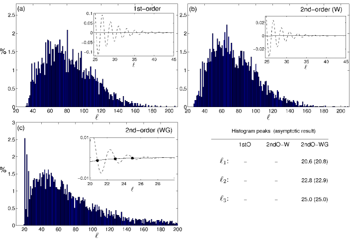
Figure 16: (Color online) Histograms of the pulse-separation distances for $\delta=1.82$ in (a) the first-order model ($\eta=0$), (b) the second-order model with the parameter values corresponding to W ($\eta=0.015$), and (c) the second-order model with the parameter values corresponding to WG ($\eta=0.052$). The table shows the numerical value of the peaks observed in the histograms compared to the values predicted by the model given by (29a), plotted in the insets of each panel, where the dashed and solid lines corresponds to the $S_{2}$ and $S_{1}$ functions, respectively.

Figure 15 shows the results for $\delta=1.28$, that corresponds to $\mbox{{Re}}=3.75$ and $2$ for W and WG, respectively. The distributions are again characterized by the presence of peaks representing the selected distances at which bound states are observed. In this case, we observe four peaks that are sharper and more pronounced in the second-order simulations than we observed before. We find that the histogram peaks obtained in the W-simulations occur at similar distances for both the first- and the second-order models, and are in very good agreement with the theory (see the table in Fig. 15). It is interesting to note, however, that such a similarity between both models is no longer observed when the simulations are made by using the parameter values for WG. In this case, the second-order effects start to become important, and the distances at which the bound states are observed change accordingly. We find that the first observed peak for the second-order model occurs at $\ell_{1}\simeq 17.4$, in contrast to the value obtained by using the first-order model, $\ell_{1}\simeq 20.9$. Also, we note that the dominant peak in the histogram for the second-order model is found at $\ell_{2}\simeq 19.9$, whereas the peak corresponding to the first-order model is found at $\ell_{3}\simeq 31$. All of these differences can be explained in terms of the decrease of the amplitude of the capillary ripples preceding the main solitary humps that is largely influence by second-order effects (cf. Fig. 2), which in turn, allows the pulses to get closer to each other. It is worth mentioning that for $\ell_{1}\approx 17.4$ the assumption of well-separated pulses is not quite satisfied and, as expected, the theoretical and numerical results are not in good agreement.

Figure 16 depicts the results for $\delta=1.82$, that corresponds to $\mbox{{Re}}=5$ and $2.66$ for W- and WG-simulations, respectively. The W-simulations reveal that there is no any clear distance selection among pulses. The distributions of the separation distances for both the first- and second-order models are broader, as compared to the previous cases and without a dominant peak. This seems to indicate that the pulses start to feel the effect of some underlying chaotic behaviour with the eventual loss of self-organisation into bound states, but unlike the spatio-temporal chaos with the KS equation, solitary pulses are still clearly identifiable. Interestingly, when the simulations are performed using the values of the parameters corresponding to WG, the consequence of including the viscous-dispersion effects due to the second-order terms becomes crucial in the bound-state formation process. Indeed, the histogram obtained for the second-order model is still dominated by the presence of three peaks which are in agreement with the theoretically predicted bound states. This is a clear evidence that viscous dispersion plays an important role in the self-organisation process that brings the system in a state which can be described in terms of bound states.

IV.3 Solitary-wave gas density

Our numerical observations for $\delta=0.98$ and $1.28$ have shown that there is a clear selection process for which the pulses self-organise to form bound states described by well-defined distances. From a statistical point of view, it is therefore reasonable that in a large domain containing many solitary waves interacting through attractions and repulsions with each other, the system can be described in terms of a mean separation distance, that gives information about the density of solitary waves. In this sense, we can treat the system as a “gas” compound of solitary waves with a well-defined density. To characterize such a solitary-wave gas, we shall assume that for long times and large spatial domains, the distribution of the separation distances between pulses is mainly dominated by the peaks observed in Figs. 14 and 15. This is a reasonable assumption considering that the peaks become more pronounced as the system evolves on time, something that has been observed in the gKS equation Tseluiko, Saprykin, and Kalliadasis (2010); Tseluiko et al. (2010), and also in our numerical experiments. We then define the mean separation distance as

$$\langle\ell\rangle=\sum_{i=1}^{n}\alpha_{i}\ell_{i},$$ (34)

where $n$ is the number of peaks of the histogram, and $\alpha_{i}$ is an average weight that we approximate as

$$\alpha_{i}=\frac{p_{i}}{\sum_{1}^{n}p_{i}},$$ (35)

where $p_{i}$ is the probability of each peak. By using this definition we can estimate the typical mean separation length between the pulses and therefore, we can obtain an estimate of the density of the solitary-wave gas by using:

$$\rho_{s}=\frac{1}{\langle\ell\rangle}.$$ (36)

	$\delta=0.98$	$\delta=1.28$
1st-order	0.036	0.034
2nd-order (W)	0.038	0.035
2nd-order (WG)	0.039	0.045

Table 1: Density $\rho_{s}$ of the solitary-wave gas for different values of $\delta$ and for the first-order model, and second-order model for both W and WG.

The densities obtained for each $\delta$ are given in Table 1. As expected, the density of the solitary-wave gas increases as the viscous-dispersion effects are taken into account. It is important to emphasize that such a density has been defined from a selected preferential mean separation length, and not from a random mean length that would arise, for instance, if the pulses were irregularly spaced. This is an important point which reflects how a quasi-turbulent system (in the sense that the pulses are continuosly and randomly interacting with each other) has an underlying ordered, or a “permanent“ self-organized state, that can be understood in terms of bound-state formation. An important feature of this state, the average separation distance between the pulses, is largely dependent on viscous-dispersion effects.

V Conclusions

We have examined both analytically and numerically the interactions of two-dimensional solitary pulses in falling liquid films. We focused in particular on the formation of bound states of pulses and how it is affected by the second-order (in the long-wave expansion parameter) viscous-dispersion effects. To this end, we made use of a second-order two-field model derived in Refs. Ruyer-Quil and Manneville, 2000, 2002. This is a system of coupled nonlinear partial differential equations for the local flow rate and the film thickness.

Our theoretical investigation of the formation of bound states was based on appropriately extending the rigorous coherent-structure theory for the gKS equation recently developed in Refs. Duprat et al., 2009; Tseluiko, Saprykin, and Kalliadasis, 2010; Tseluiko et al., 2010 to the second-order two-field model (and thus putting the coherent-structure theory for falling films on a rigorous basis). By assuming that the solution is given by a superposition of $N$ pulses and a small overlap (correction) function, i.e. assuming that the pulses are well separated (weak interaction), we were able to write down a dynamic equation for the overlap function in the vicinity of each pulse, that is described by a linear matrix/differential operator and contains forcing terms due to the neighboring pulses. A careful and detailed analysis of the spectral properties of the linear operator revealed that the relevant eigenfunction is the translational mode that corresponds to the zero eigenvalue. This eigenvalue is not isolated and, therefore, belongs to the essential spectrum. The null space of the adjoint operator is spanned by a constant vector function and another non-constant function that has an infinite norm, meaning that zero is not in the point spectrum of the adjoint operator. This spectral behavior is similar to the one observed for the gKS equation Tseluiko, Saprykin, and Kalliadasis (2010); Tseluiko et al. (2010). Projections to the translational mode were made rigorous by using formulation in a weighted space. The outcome of the projections is a dynamical system for the pulse locations. By studying its fixed points, we were able to predict the distances at which the bound states are formed.

Numerical experiments of the temporal evolution of a superposition of two pulses have been found in very good agreement with the theoretical predictions, and in particular, the theoretically predicted attractive and repulsive dynamics that gives rise to the formation of bound states. We demonstrated that the second-order viscous-dispersion terms are crucial for an accurate description of the pulse interactions. These terms affect the amplitude and frequency of the capillary ripples in front of a solitary pulse. So their influence is in fact linear, but interestingly they can have some crucial consequences on the nonlinear dynamics of the film and the wave-selection process in the spatio-temporal evolution. After all, solitary pulses interact through their tails which overlap, i.e. the capillary ripples and their amplitude and frequency will affect the separation distance between the pulses: for example, smaller-amplitude ripples will allow for more overlap between the tails of neighboring pulses, thus decreasing their separation distance. This in turn will affect the average separation distance between pulses when the system reaches its permanent quasi-turbulent regime and hence the density of the solitary waves. This also means that any model that does not include second-order terms should be used with caution and certainly not for an accurate description of solitary pulse interaction which dominates the spatio-temporal dynamics of the film.

In addition, we have studied strong interaction between two pulses and found that it leads to an oscillatory behavior of the separation length as was also numerically observed in Ref. Malamataris, Vlachogiannis, and Bontozoglou, 2002 from direct numerical simulations of full Navier–Stokes equations and wall and free-surface boundary conditions. This behavior escapes the description of our weak-interaction theory. Again, we find that viscous dispersion effects are crucial and the strong nonlinear interaction between pulses can be largely reduced by increasing the viscous-dispersion parameter.

We have also performed numerical simulations in extended domains with a localized random initial condition. These allowed us to study the interaction between the pulses and how they self-organize to form bound states in extended domains. Detailed statistical analysis of the pulse separation distances revealed that the histograms of the separation distances have clear peaks that correspond to the theoretically predicted bound states. We have used different values of the reduced Reynolds number $\delta$ and two different sets of physical parameters corresponding to two liquids of different viscosities, namely water and a mixture of water and glycerin. In all cases, we have observed that the peaks of the histograms corresponding to the shortest distances are always more pronounced in the second-order simulations. As expected, the differences between the first- and the second-order models were found to be more important in the case of the higher viscosity liquid. We observed that the minimum distance at which bound states are formed is always shorter in the second-order simulations. It is important to note that in the cases of $\delta=0.98$ and $1.28$, both models have shown that there is always formation of bound states, indicating that statistically, the free surface can be treated as a solitary-wave gas, characterized by a typical constant mean distance between the pulses.

Of particular interest would be the extension of the coherent structures theory developed here to other viscous flow problems, for example the problem of a thin film coating a vertical fiber (e.g Kalliadasis and Chang, 1994; Duprat et al., 2007; Ruyer-Quil et al., 2008) in which case due to the Rayleigh–Plateau instability the film breaks up into a train of droplike solitary waves. The recent experiments in Ref. Ruyer-Quil et al., 2008 indicate clearly the formation of bound states in a region of the parameter space where the Rayleigh–Plateau instability competes with viscous dispersion. The qualitative agreement between the experiments and the coherent-structure theory developed in Refs. Tseluiko, Saprykin, and Kalliadasis, 2010; Tseluiko et al., 2010 is encouraging. Our hope is that quantitative agreement can be achieved by extending the present theory to the second-order model for flow down a fiber developed in Ref. Ruyer-Quil et al., 2008. For that matter, the present formalism could be extended to other two-equation systems, e.g. coupled KS-type equations used to describe synchronization phenomena Tasev et al. (2000).

Finally, as noted in the Introduction, the two-dimensional pulses considered here are only observed up to a certain, low-to-moderate, value of the Reynolds number. At higher Reynolds numbers, two-dimensional pulses develop an instability in the transverse direction and a transition to a fully developed three-dimensional regime is observed (e.g. Demekhin et al., 2007a, b). The coherent-structure theory developed here can be viewed as a foundation first step for the analysis of the interactions between three-dimensional pulses in falling films.

Appendix A The adjoint operators

The adjoint operator $\boldsymbol{\mathcal{L}}_{i}^{*}$ is defined as

$$\langle\boldsymbol{u},\boldsymbol{\mathcal{L}}_{i}\boldsymbol{v}\rangle=\langle\boldsymbol{\mathcal{L}}_{i}^{*}\boldsymbol{u},\boldsymbol{v}\rangle,$$ (37)

where $\langle\cdot,\cdot\rangle$ denotes the usual inner product in $L_{\mathbb{C}}^{2}$ given by

$$\langle\boldsymbol{u},\boldsymbol{v}\rangle=\int_{-\infty}^{\infty}\!\!\!\!\!\boldsymbol{u}^{T}\!\cdot\overline{\boldsymbol{v}}\,\mathrm{d}x.$$ (38)

After integration by parts, we find that the adjoint operator is

$$\boldsymbol{\mathcal{L}}_{i}^{*}=\begin{pmatrix}\mathcal{L}_{i}^{*1}&\mathcal{L}_{i}^{*2}\\ \mathcal{L}_{i}^{*3}&\mathcal{L}_{i}^{*4}\end{pmatrix},$$ (39)

with components

$$\mathcal{L}_{i}^{*1} = -\frac{5}{2\delta}\frac{1}{h_{i}^{2}}+\frac{1}{7}\frac{q_{i}}{h_{i}^{2}}h_{ix}-\bigg{(}c_{0}-\frac{17}{7}\frac{q_{i}}{h_{i}}\bigg{)}\partial_{x}{}$$

$$+\frac{\eta}{\delta}\bigg{(}-\frac{3}{2}\frac{h_{ix}^{2}}{h_{i}^{2}}-\frac{1}{2}\frac{h_{ixx}}{h_{i}}+\frac{9}{2}\frac{h_{ix}}{h_{i}}\partial_{x}+\frac{9}{2}\partial_{xx}\bigg{)},{}$$

$$\mathcal{L}_{i}^{*2} = \partial_{x}{}$$

$$\mathcal{L}_{i}^{*3} = \frac{5}{6\delta}+\frac{5}{\delta}\frac{q_{i}}{h_{i}^{3}}-\frac{1}{7}q_{i}\frac{q_{ix}}{h_{i}^{2}}+\frac{9}{7}\frac{q_{i}^{2}}{h_{i}^{2}}\partial_{x}-\frac{5}{2\delta}h_{ix}\partial_{xx}{}$$

$$-\frac{5}{6\delta}h_{i}\partial_{xxx}+\frac{\eta}{\delta}\bigg{[}4q_{ix}\frac{h_{ix}}{h_{i}^{2}}-4q_{i}\frac{h_{ix}^{2}}{h_{i}^{3}}+4q_{i}\frac{h_{ixx}}{h_{i}^{2}}{}$$

$$-\frac{3}{2}\frac{q_{ixx}}{h_{i}}-\bigg{(}20q_{i}\frac{h_{ix}}{h_{i}^{2}}+\frac{15}{2}\frac{q_{ix}}{h_{i}}\bigg{)}\partial_{x}-6\frac{q_{i}}{h_{i}}\partial_{xx}\bigg{]},{}$$

$$\mathcal{L}_{i}^{*4} = -c_{0}\partial_{x}.$$

The spectrum of the adjoint operator is shown in Fig. 17.

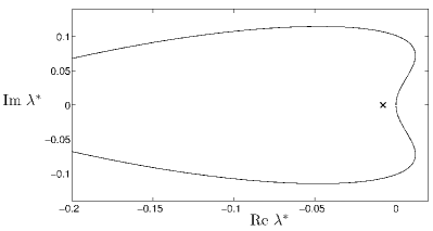
Figure 17: Spectrum of $\boldsymbol{\mathcal{L}}_{i}^{*}$ on an infinite domain for $\delta=0.98$ with the physical parameters corresponding W. The solid line is the locus of the essential spectrum and the cross represents the point spectrum.

In addition, it is straightforward to see that on a periodic domain the zero eigenfunction is a constant:

$${\boldsymbol{\Psi}}_{1}^{i}=\binom{0}{m},$$ (40)

so that $\boldsymbol{\mathcal{L}}_{i}^{*}{\boldsymbol{\Psi}}_{1}^{i}=0$. As shown in Fig. 7($b$), on an infinite domain we have $m\to 0$ and therefore there is no such a function in the null space of the adjoint operator that also belongs to $L_{\mathbb{C}}^{2}$. We can therefore conclude that zero is not in the point spectrum of $\boldsymbol{\mathcal{L}}_{i}^{*}$. The generalized zero eigenfunction on a periodic domain, i.e. the function satisfying $\boldsymbol{\mathcal{L}}_{i}^{*}{\boldsymbol{\Psi}}_{2}^{i}={\boldsymbol{\Psi}}_{1}^{i}$, is found numerically and its components are shown in Fig. 6.

We can also show that the adjoint operator $\boldsymbol{\mathcal{J}}_{i}^{*}$ is:

$$\boldsymbol{\mathcal{J}}_{i}^{*}=\begin{pmatrix}\mathcal{J}_{i}^{*1}&0\\ \mathcal{J}_{i}^{*2}&0\end{pmatrix}$$ (41)

with components:

$$\mathcal{J}_{i}^{*1} = \frac{18q_{i}}{7h_{i}^{2}}H_{ix}+\frac{17}{7h_{i}}\bigg{(}\frac{Q_{i}H_{ix}}{h_{i}}+Q_{i}\partial_{x}\bigg{)}{}$$

$$+\frac{\eta}{2\delta}\bigg{(}\frac{17}{h_{i}^{2}}H_{ix}^{2}-\frac{21}{h_{i}}H_{ixx}+\frac{9}{h_{i}}H_{ix}\partial_{x}\bigg{)},{}$$

$$\mathcal{J}_{i}^{*2} = \frac{5}{\delta h_{i}^{4}}(q_{i}H_{i}+Q_{i})-\frac{1}{7h_{i}^{2}}\bigg{(}q_{i}Q_{ix}+\frac{H_{ix}}{h_{i}}\bigg{)}{}$$

$$-\bigg{(}\frac{5}{2\delta}H_{ixx}+\frac{9q_{i}^{2}-1}{7h_{i}^{2}}\bigg{)}\partial_{x}-\frac{5}{2\delta}H_{ix}\partial_{xx}{}$$

$$-\frac{5}{6\delta}H_{i}\partial_{xxx}+\frac{\eta}{\delta}\bigg{[}\frac{4}{h_{i}^{2}}\bigg{(}Q_{ix}H_{ix}-\frac{q_{i}H_{ix}^{2}}{h_{i}}+\frac{H_{ix}^{2}}{h_{i}}{}$$

$$+q_{i}H_{ixx}-\frac{H_{ixx}}{2}-\frac{3}{4}h_{i}Q_{ix}\bigg{)}+\bigg{(}\frac{4Q_{i}H_{ix}}{h_{i}^{2}}+{}$$

$$\frac{8}{3}\frac{H_{ix}}{h_{i}^{2}}-\frac{15}{2}\frac{Q_{ix}}{h_{i}}\bigg{)}\partial_{x}-\frac{6}{h_{i}}Q_{i}\partial_{xx}\bigg{]}.$$

References

- Kapitza (1948a) P. L. Kapitza, “Wave flow of thin layers of viscous fluid: I. Free flow,” Zh. Eksp. Teor. Fiz. 18, 3–18 (1948a).
- Kapitza (1948b) P. L. Kapitza, “Wave flow of thin layers of a viscous fluid: II. Fluid flow in the presence of continuous gas flow and heat transfer,” Zh. Eksp. Teor. Fiz. 18, 19–28 (1948b).
- Kapitza and Kapitza (1949) P. L. Kapitza and S. P. Kapitza, “Wave flow of thin layers of a viscous fluid: III. Experimental study of undulatory flow conditions,” Zh. Eksp. Teor. Fiz. 19, 105–120 (1949).
- Chang (1994) H.-C. Chang, “Wave evolution on a falling film,” Annu. Rev. Fluid Mech. 26, 103–136 (1994).
- Chang and Demekhin (2002) H.-C. Chang and E. Demekhin, Complex Wave Dynamics on Thin Films (Springer, Elsevier; Amsterdam, 2002).
- Kalliadasis and Thiele (2007) S. Kalliadasis and U. Thiele, eds., Thin Films of Soft Matter (Springer-Wien, New York, 2007).
- Demekhin et al. (2007a) E. A. Demekhin, E. N. Kalaidin, S. Kalliadasis, and S. Y. Vlaskin, “Three-dimensional localized coherent structures of surface turbulence. I. Scenarios of two-dimensional–three-dimensional transition,” Phys. Fluids 19, 114103 (2007a).
- Krantz and Goren (1971) W. B. Krantz and S. L. Goren, “Stability of thin liquid films flowing down a plane,” Ind. Eng. Chem. Fundam. 10, 91–101 (1971).
- Liu and Gollub (1993) J. Liu and J. P. Gollub, “Onset of spatially chaotic waves on flowing films,” Phys. Rev. Lett. 70, 2289–2292 (1993).
- Liu, Paul, and Gollub (1993) J. Liu, J. D. Paul, and J. P. Gollub, “Measurements of the primary instabilities of film flows,” J. Fluid Mech. 250, 69–101 (1993).
- Vlachogiannis and Bontozoglou (2001) M. Vlachogiannis and V. Bontozoglou, “Observations of solitary wave dynamics of film flows,” J. Fluid Mech. 435, 191–215 (2001).
- Argyriadi, Serifi, and Bontozoglou (2004) K. Argyriadi, K. Serifi, and V. Bontozoglou, “Nonlinear dynamics of inclined films under low-frequency forcing,” Phys. Fluids 16, 2457–2468 (2004).
- Pumir, Manneville, and Pomeau (1983) A. Pumir, P. Manneville, and Y. Pomeau, “On solitary waves running down an inclined plane,” J. Fluid Mech. 135, 27–50 (1983).
- Chang, Demekhin, and Kalaidin (1995) H.-C. Chang, E. Demekhin, and E. Kalaidin, “Interaction dynamics of solitary waves on a falling film,” J. Fluid Mech. 294, 123–154 (1995).
- Chang, Demekhin, and Saprykin (2002) H.-C. Chang, E. A. Demekhin, and S. S. Saprykin, “Noise-driven wave transitions on a vertically falling film,” J. Fluid Mech. 462, 255–283 (2002).
- Duprat et al. (2009) C. Duprat, F. Giorgiutti-Dauphiné, D. Tseluiko, S. Saprykin, and S. Kalliadasis, “Liquid film coating a fiber as a model system for the formation of bound states in active dispersive–dissipative nonlinear media,” Phys. Rev. Lett. 103, 234501 (2009).
- Ruyer-Quil and Manneville (1998) C. Ruyer-Quil and P. Manneville, “Modeling film flows down inclined planes,” Eur. Phys. J. B 6, 277–292 (1998).
- Ruyer-Quil and Manneville (2000) C. Ruyer-Quil and P. Manneville, “Improved modeling of flows down inclined planes,” Eur. Phys. J. B 15, 357–369 (2000).
- Ruyer-Quil and Manneville (2002) C. Ruyer-Quil and P. Manneville, “Further accuracy and convergence results on the modeling of flows down inclined planes by weighted-residual approximations,” Phys. Fluids 14, 170–183 (2002).
- Tseluiko, Saprykin, and Kalliadasis (2010) D. Tseluiko, S. Saprykin, and S. Kalliadasis, “Interaction of solitary pulses in active dispersive-dissipative media,” Proc. Est. Acad. Sci. 59, 139–144 (2010).
- Tseluiko et al. (2010) D. Tseluiko, S. Saprykin, C. Duprat, F. Giorgiutti-Dauphiné, and S. Kalliadasis, “Pulse dynamics in low-Reynolds-number interfacial hydrodynamics: Experiments and theory,” Physica D 239, 2000–2010 (2010).
- Balmforth (1995) N. J. Balmforth, “Solitary waves and homoclinic orbits,” Annu. Rev. Fluid Mech. 27, 335–373 (1995).
- Ei (2002) S.-I. Ei, “The motion of weakly interacting pulses in reaction-diffusion systems,” J. Dynam. Differential Equations 14, 85–137 (2002).
- Zelik and Mielke (2009) S. Zelik and A. Mielke, “Multi-pulse evolution and space-time chaos in dissipative systems,” Mem. Amer. Math. Soc. 198, 1–95 (2009).
- Elphick et al. (1991) C. Elphick, G. R. Ierley, O. Regev, and E. A. Spiegel, “Interacting localized structures with Galilean invariance,” Phys. Rev. A 44, 1110–1122 (1991).
- Ei and Ohta (1994) S.-I. Ei and T. Ohta, “Equation of motion for interacting pulses,” Phys. Rev. E 50, 4672–4678 (1994).
- Oron, Davis, and Bankoff (1997) A. Oron, S. H. Davis, and S. G. Bankoff, “Long-scale evolution of thin liquid films,” Rev. Mod. Phys. 69, 931–980 (1997).
- Benney (1966) D. J. Benney, “Long waves on liquid films,” J. Math. Phys. 45, 150–155 (1966).
- Shkadov (1977) V. Ya. Shkadov, “Solitary waves in a layer of viscous liquid,” Izv. Akad. Nauk SSSR, Mekh. Zhidk. Gaza 1, 63–66 (1977).
- Shkadov (1967) V. Y. Shkadov, “Wave modes in the flow of thin layer of a viscous liquid under the action of gravity,” Izv. Akad. Nauk SSSR, Mekh. Zhidk Gaza 1, 43–50 (1967).
- Pego and Weinstein (1994) R. L. Pego and M. I. Weinstein, “Asymptotic stability of solitary waves,” Commun. Math. Phys. 164, 305–349 (1994).
- Sandstede and Scheel (2000) B. Sandstede and A. Scheel, “Absolute and convective instabilities of waves on unbounded and large bounded domains,” Physica D 145, 233–277 (2000).
- Malamataris, Vlachogiannis, and Bontozoglou (2002) N. A. Malamataris, M. Vlachogiannis, and V. Bontozoglou, “Solitary waves on inclined films: Flow structure and binary interactions,” Phys. Fluids 14, 1082–1095 (2002).
- Savva, Kalliadasis, and Pavliotis (2010) N. Savva, S. Kalliadasis, and G. A. Pavliotis, “Two-dimensional droplet spreading over random topographical substrates,” Phys. Rev. Lett. 104, 084501–084504 (2010).
- Kalliadasis and Chang (1994) S. Kalliadasis and H.-C. Chang, “Drop formation during coating of vertical fibres,” J. Fluid Mech. 261, 135–168 (1994).
- Duprat et al. (2007) C. Duprat, C. Ruyer-Quil, S. Kalliadasis, and F. Giorgiutti-Dauphiné, “Absolute and convective instabilities of a film flowing down a vertical fiber,” Phys. Rev. Lett. 98, 244502 (2007).
- Ruyer-Quil et al. (2008) C. Ruyer-Quil, P. M. J. Trevelyan, F. Giorgiutti-Dauphiné, C. Duprat, and S. Kalliadasis, “Modelling film flows down a fiber,” J. Fluid Mech. 603, 431–462 (2008).
- Tasev et al. (2000) Z. Tasev, L. Kocarev, L. Junge, and U. Parlitz, “Synchronization of Kuramoto-Sivashinsky equations using spatial local coupling,” Int. J. Bifurcat. Chaos 10, 869–873 (2000).
- Demekhin et al. (2007b) E. A. Demekhin, E. N. Kalaidin, S. Kalliadasis, and S. Y. Vlaskin, “Three-dimensional localized coherent structures of surface turbulence. II. solitons,” Phys. Fluids 19, 114104 (2007b).