Homologous Flares and Magnetic Field Topology in Active Region NOAA 10501 on 20 November 2003

Abstract

We present and interpret observations of two morphologically homologous flares that occurred in active region (AR) NOAA 10501 on 20 November 2003. Both flares displayed four homologous H$\alpha$ ribbons and were both accompanied by coronal mass ejections (CMEs). The central flare ribbons were located at the site of an emerging bipole in the center of the active region. The negative polarity of this bipole fragmented in two main pieces, one rotating around the positive polarity by $\approx 110^{\circ}$ within 32 hours. We model the coronal magnetic field and compute its topology, using as boundary condition the magnetogram closest in time to each flare. In particular, we calculate the location of quasi-separatrix layers (QSLs) in order to understand the connectivity between the flare ribbons. Though several polarities were present in AR 10501, the global magnetic field topology corresponds to a quadrupolar magnetic field distribution without magnetic null points. For both flares, the photospheric traces of QSLs are similar and match well the locations of the four H$\alpha$ ribbons. This globally unchanged topology and the continuous shearing by the rotating bipole are two key factors responsible for the flare homology. However, our analyses also indicate that different magnetic connectivity domains of the quadrupolar configuration become unstable during each flare, so that magnetic reconnection proceeds differently in both events.

1 Introduction

Solar flares involve a sudden energy release in a restricted volume of the solar corona, occurring on time scales of minutes up to a few hours. Confined flares take place in loops in the lower corona and the emission largely comes from the plasma in those loops. Eruptive flares, on the other hand, are typically associated with a coronal mass ejection (CME) and often occur in conjunction with a filament eruption. It is now widely accepted that these three phenomena (eruptive flare, CME, and filament eruption) are different observational manifestations of a sudden and violent disruption of the coronal magnetic field, often simply referred to as “solar eruption” (see, e.g., Forbes00). Whether or not all three phenomena occur together appears to depend mainly on details of the pre-eruptive configuration. Cases in which the eruption does not evolve into a CME are called “failed eruption” (see, e.g., Torok05).

The so-called CSHKP model for eruptive flares was put forward by Carmichael64, Sturrock66, Hirayama74, and Kopp76 and has been refined by many authors since then. This model provides explanations for all main observational flare features, as for example the formation and separation of ribbons. However, it does not address the detailed mechanisms by which eruptions are triggered and driven, which still belong to the most lively discussed problems in solar physics. Accordingly, a large variety of theoretical models for the initiation of eruptions has been proposed in the last decades (for a recent comprehensive review, see the Introduction in Aulanier10). Among these models are the “tether-cutting model” (hereafter TC; see, e.g., Moore92; Moore01) and the “magnetic breakout model” (hereafter MB; see, e.g., Antiochos98; Antiochos99). In the following, we briefly describe these two models since they appear to be consistent with the observations presented in this paper.

In the TC model, the eruption starts by the interaction of two low-lying sheared arcades located in a bipolar area in an AR. If these arcades come into contact, for example due to photospheric motions, they start to reconnect and progressively form a magnetic flux rope. After the stabilizing influence of the magnetic field overlying the newly formed flux rope has been sufficiently weakened by the reconnection below it (hence the term “tether cutting”), the flux rope erupts, evolving into a CME or into a failed eruption (see Figure 1 in Moore01). Although formulated for a bipolar configuration, the model works also if the bipole is part of a larger multipolar active region [Moore and Sterling (2006)].

In the MB model, the eruption is initiated at a magnetic null point (or null line) located above a sheared magnetic arcade in a quadrupolar configuration. If the arcade starts to rise, for example due to further shearing by photospheric motions, its expansion triggers current sheet formation and reconnection at the null point. The reconnection progressively decreases the magnetic tension of the overlying magnetic field, allowing the arcade to erupt. The expansion of the arcade leads to the formation of a flux rope that erupts as part of the arcade.

We note that both models do not directly address the physical mechanism by which the flux rope eruption is driven. This mechanism is most likely a “catastrophic loss of equilibrium” or the ideal MHD (“torus”) instability related to it (e.g., for91; kli06; Aulanier10).

Both the TC and MB models predict a slow reconnection process in the initial phase of the eruption and a fast one in its main phase. The latter takes place below the erupting flux and yields two main ribbons, in agreement with the CSHKP model. The initial reconnection, however, occurs below the erupting flux in a bipolar configuration in the TC model and above it in a quadrupolar configuration in the MB model. As a consequence, the expected pattern of brightenings in the pre-flare phase is different. Both models predict the simultaneous appearance of four brightenings in this phase. In the TC model, these are located within a bipolar area, pairwise at each side of the polarity inversion line (PIL, see Figure 1 in Moore01). In the MB model, they are located at alternating polarities, within a quadrupolar area of the photospheric magnetic field.

To set constrains on the energy release mechanism and initiation process during flares, it is helpful to combine the analysis of the morphology and temporal evolution of the event with the computation of the magnetic topology of the AR where it occurs (e.g., Demoulin07; Mandrini10). Active region magnetic fields can contain separatrices and, more generally, quasi-separatrix layers (QSLs). Separatrices are locations where the connectivity of magnetic field lines is discontinuous. They are formed by field lines that either pass through a null point or through a bald-patch neutral line (defined by field lines tangent to the photosphere at a PIL). QSLs are a generalization of separatrices; they are defined as regions where the connectivity of magnetic field lines changes drastically, but can be continuous (Priest95; Demoulin96a; Demoulin96). The relationship between separatrices/QSLs in 3D and observations has been explored for a large variety of solar magnetic configurations. H$\alpha$ and UV flare ribbons have been found along, or next to, the photospheric or chromospheric traces of QSLs [Démoulin et al. (1997), Mandrini et al. (1997), Bagalá et al. (2000), Masson et al. (2009)]. In addition, electric current concentrations were found along the photospheric traces of QSLs [Démoulin et al. (1997), Mandrini et al. (1997)]. The release of free magnetic energy, associated with these currents, can occur at QSLs when their thickness, and that of their associated current layers, is small enough for reconnection to take place, as recently shown by MHD simulations of flare-like magnetic configurations (Aulanier05; Aulanier06b).

Occasionally flares and CMEs can occur in the same AR within minutes or hours. If such events exhibit a similar morphology, for example similar locations and shapes of flare brightenings, they are called homologous. This repetitive character of flares was first discussed by Waldmeier38. Definitions of homologous flaring include similarities in H$\alpha$ or EUV brightenings, in soft X-ray structures, and/or radio bursts with similar dynamic spectra (e.g., Woodgate84; Machado85; Martres89). Homologous flares are particularly interesting phenomena since they pose some challenging questions about the conditions that lead to flaring: do they occur since not all of the available free magnetic energy is released or because free energy is continuously supplied to the AR (see, e.g., Bleybel02; Schrijver09)? A quantitative study of homologous flares is presented by takasaki04. In particular, they found that the separation velocity of the flare ribbons has a good correlation with the soft X-ray light curve, and they derived a similar coronal magnetic field strength for three homologous flares, a result which support magnetic reconnection for the energy release mechanism. Moreover, recent numerical simulations have demonstrated that eruptions can indeed occur repeatedly if flux continues to emerge into the corona [MacTaggart and Hood (2009)], or if the coronal magnetic field is continuously sheared by photospheric motions [DeVore and Antiochos (2008)].

On the other hand, the fact that homologous flares are morphologically similar is an indication of the key role played by the magnetic field topology (including QSLs), since it is mainly determined by the global distribution of the photospheric polarities (see examples in Machado88; Mandrini91, 1997). However, though morphologically similar, some homologous flares can produce different soft X-ray light curves, implying differences in the impulsiveness of energy release (Ranns00; Sterling01)

In this paper we study observations of two homologous flares that occurred in AR NOAA 10501 on 20 November 2003. A multi-wavelength study of these events, including the associated filament evolution and CMEs, and an analysis of a magnetic cloud associated with the second event, was recently presented by Kumar09. Here we focus on the flare evolution, morphology, and homology, and we compare our interpretation of the two events with the interpretation by Kumar09. While these authors attributed the flare trigger for both events to the dynamic interaction of two filaments, we rather believe that an emerging and rotating bipole in the center of the AR was at the origin of the observed eruptive activity.

A summary of the events and a description of the analyzed data are presented in Section 2. The observational details of both flares and the evolution of the photospheric magnetic field are described in Section 3. Section 4 presents the magnetic field model and topology of the AR, together with a possible explanation for the evolution and morphology of the flares. Finally, we present our conclusions in Section 5.

Figure 1.: Temporal evolution of the solar soft X-ray flux as observed by GOES 12 in the 0.5-4 Å and 1-8 Å bandwidths on 20 November 2003. The two studied flares, occurring in AR 10501, are pointed at by arrows. The M1.4 event occurred at 02:12 UT and the M9.6 at 07:45 UT. The C4.3 event at $\approx$ 04:32 UT occurred in AR 10508.

2 Summary of the Activity in AR 10501 and Observational Data

2.1 Activity in AR 10501 on 20 November 2003

Active region NOAA 10501 was one of the most complex and eruptive regions during the decay phase of solar cycle 23. This AR was the successor of the also very flare productive active region NOAA 10484, as it was named during the previous solar rotation. AR 10501 produced 12 M-class flares, some of them accompanied by CMEs, from 18 to 20 November 2003. In particular, the early events on 18 November 2003 have been extensively studied (gopalswamy05; Yurchyshyn05; Mostl08; Srivastava09; Chandra10). The peculiarity of this AR on that day was that it contained regions of different magnetic helicity signs, as was discussed by Chandra10. This characteristic seems to be present also on 20 November 2003 (see Section 4).

On 20 November 2003, two homologous flares took place within approximately five hours in the region, which was located around N03 W05 at that time (see Section 3). The flares were, respectively, classified as M1.4 and M9.6 from the GOES soft X-ray emission (Figure 1). The first flare (M1.4) was preceded by a pre-flare phase starting at $\approx$ 01:30 UT. Its main phase started at 01:45 UT with a relatively gradual onset, peaked at 02:12 UT, and ended around 02:40 UT. The flare was accompanied by a very dynamic behaviour of the AR filaments and by a CME (see Section 3.2.3 for details).

The second flare was preceded by a weak (C3.8) precursor starting at around 7:25 UT. The flare main phase began with an impulsive onset at 07:35 UT, peaked at 07:45 UT, and reached class M9.6. Finally, the flare ended gradually at around 08:40 UT. This flare was accompanied by successive filament eruptions and by a CME (see Section 3.3.2 for details.)

Though the flares were morphologically similar, the soft X-ray GOES light curve indicates a more gradual energy release during the first flare than during the second one. Another flare (of C-class) started at $\approx$ 4:32 UT (Figure 1). However, it was located in another region (AR 10508). Just after this flare, around 5:12 UT, a small flare was occuring in AR 10501 (see the small peak in Figure 1). This flare took place at the same location, and displayed similar ribbons, as the M1.4 and M9.6 flares (see the EIT 195 Å observations at http://www.ias.u-psud.fr/eit/movies/). Around 23:47 UT, another homologous flare occurred, indicating that the magnetic configuration of AR 10501 was still similar. We do not analyze these two flares because of the lack of H$\alpha$ data and because of the low cadence of the EIT data (at best 12 min in 195 Å).

2.2 The Analyzed Data

For our study, we mainly use H$\alpha$ data from the Aryabhatta Research Institute of Observational Sciences (ARIES) in Nainital, India. These data were obtained by a 15-cm f/15 coudé telescope (pixel size 1^′′) and a Lyot filter centered at the H$\alpha$ line Uddin et al. (2004). The cadence of the H$\alpha$ images varies from 30 s to 5 min. Furthermore, we use data from the Solar and Heliospheric Observatory/Michelson Doppler Imager (SOHO/MDI; Scherrer95) with a pixel size of 1.98^′′ and a cadence of 96 minutes. The H$\alpha$ data were co-aligned with MDI magnetograms by comparing them with white-light images from SOHO/MDI.

We complement our analysis with reconstructed images from the Reuven Ramaty High-Energy Solar Spectroscopic Imager (RHESSI; Lin02), which partly observed the first flare. We reconstructed the images in the 20-60 keV energy band from seven collimators (3F to 9F) using the CLEAN algorithm, which yields a spatial resolution of $\approx 7^{\prime\prime}$ Hurford et al. (2002).

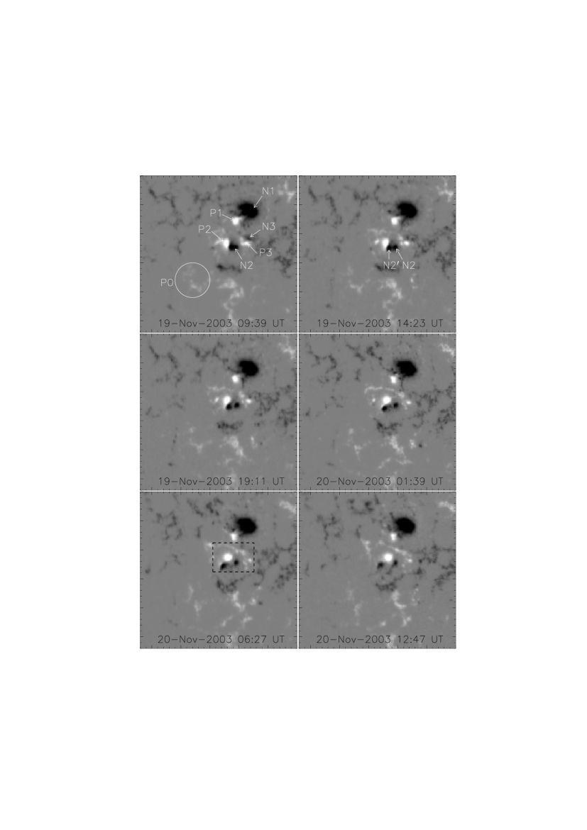
Figure 2.: Evolution of the line-of-sight magnetic field on 19 and 20 November 2003. The dashed box in the bottom left panel shows the region where N$2^{\prime}$ rotates around P2. P0 marks the positive polarity network between the two filaments (see Figure 5a). The field of view of the images is the same as in Figure 4

     

Figure 3.: Temporal evolution of the rotation angle ($\widehat{\rm N2P2N2^{\prime}}$ in degrees) of N2^′ around P2 (see Figure 2). The vertical lines show the peak times of the first and second flares, respectively.

3 Photospheric Field and Chromospheric Flare Evolution

3.1 Evolution of the Photospheric Magnetic Field

Figure 2 presents the evolution of the magnetic field on 19 and 20 November 2003, before, during and after the flares. We have numbered the six observed main polarities P1, P2, P3 (positive polarities) and N1, N2, N3 (negative polarities) in the upper left panel of Figure 2. We notice a strong diffusion of the magnetic field around the main negative polarity N1 (which is also the main spot, see the accompanying MDI movie, ar10501-mdi.mpg). The bipole N2, P2 in the central part of the active region was already visible on 15 November, when the region arrived at the eastern limb. As visible in Figure 2 (and in the MDI movie), the negative polarity N2 broke into two main pieces, which we named N2 and N2^′ in the top right panel. After the breaking, N2 remained almost at the same location, while N2^′ rotated around P2. Many other smaller negative fragments rotated as well, some preceding, some following N2^′. By computing the centroid location of N2, P2, and N2^′, we measured the rotation angle $\widehat{\rm N2P2N2^{\prime}}$. The temporal variation of this angle is shown in Figure 3 from 19 November at 06:27 UT to 20 November at 20:51 UT. The angle started increasing at 09:39 UT on 19 November and it reached $\approx$ 110^∘ at 17:39 UT on 20 November, after which the rotation ceased. Both flares studied in this paper took place during this rotation period of 32 hours.

This continuous rotation is likely to have increased the magnetic field shear along the magnetic inversion line between the polarities P2 and N2^′, and hence the free magnetic energy available for flaring. This is supported by the Marshall Space Flight Center magnetic vector data obtained on 19 November at 19:36 UT. The shear map, shown in Figure 10 of Kumar09, indicates that one of the locations of highest shear angle is along the PIL between N2+N2^′ and P2. The clockwise rotation of N2^′ around P2 implies the injection of negative magnetic helicity into the configuration.

In addition, one observes a general pattern of dispersion and cancelation of numerous small negative polarities with positive polarities of the network at the periphery of the AR in the south-west (see the MDI movie). This implies that the disperse positive polarity of the network (P0, see Figure 2) progressively shrunk both in magnetic flux and surface extension.

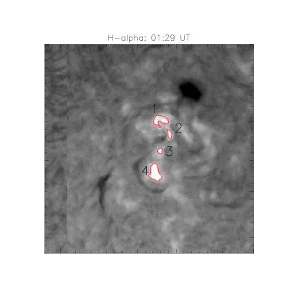
Figure 4.: (a): H$\alpha$ image during the pre-flare phase of the M1.4 event. Four brightenings are numbered as 1-4 and framed in red (by eye). (b): MDI magnetogram around the same time, overlaid with the locations of the brightenings. The field of view of the images is 270${}^{\prime\prime}\times$270^′′.

3.2 The M1.4 Class Flare

3.2.1 Chromospheric Evolution

During the pre-flare phase of the M1.4 event, at $\approx$ 01:30 UT (Figure 1), the H$\alpha$ data reveal four small brightenings, numbered as 1-4 in Figure 4. Comparing the locations of these brightenings with the MDI line-of-sight magnetogram (Figure 4b), we see that brightenings 1 and 2 are located in positive field regions, whereas 3 and 4 are located in negative field regions, on opposite sides of the local PIL. The location of the brightenings, together with their appearance before the impulsive phase, the photospheric rotation of the negative polarity N2^′, and the presence of highly sheared magnetic field, described in Section 3.1, suggest that the flare and subsequent CME (see Section 3.2.3) have been triggered as proposed by the TC model (see Section 1). A similar emission pattern in the early phase of the X10 flare on 29 October 2003 has been recently reported by Xu10.

         

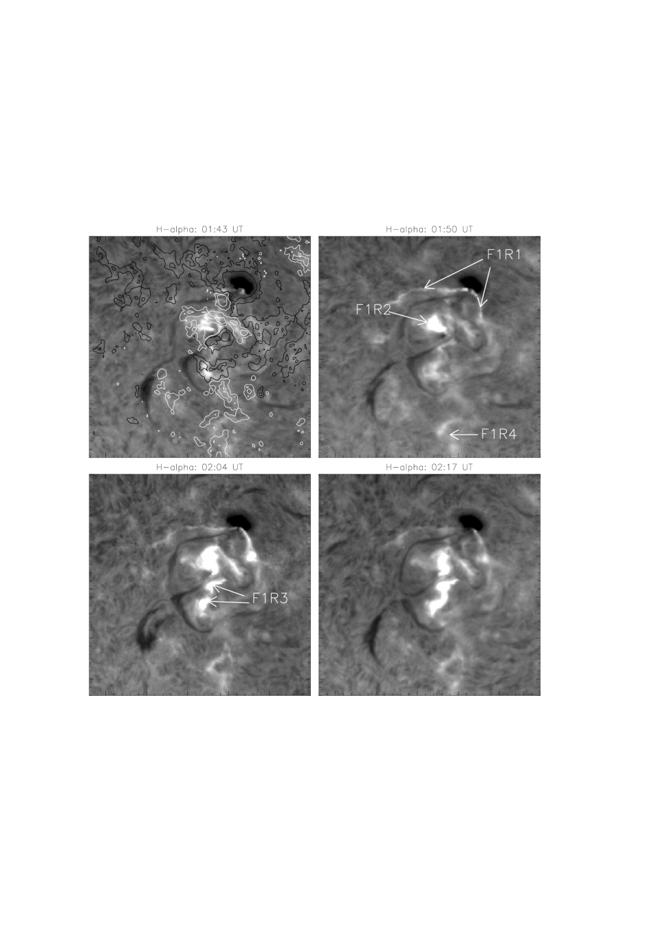
Figure 5.: H$\alpha$ evolution of the M1.4 flare. The flare ribbons are marked as F1R1, F1R2, F1R3, and F1R4, respectively. The top left panel shows overplotted contours of the photospheric line-of-sight (LOS) magnetic field at 01:39 UT. White (black) contours correspond to positive (negative) fields. Contour levels $\pm 100$ and $\pm 500$ G are used. The field of view of the images is the same as in Figure 4.

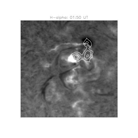
Figure 6.: H$\alpha$ image (a) and MDI magetogram (b), overlaid by RHESSI hard X-ray (20-60 keV) contours (contour levels are 40, 60, and 80$\%$ of the peak intensity). The field of view of the images is the same as in Figure 4.

The chromospheric evolution of the flare during its main phase is shown in Figure 5. Four distinct ribbons are visible: two main, inner ribbons F1R2 and F1R3, and two fainter, outer ribbons F1R1 and F1R4. Comparing Figures 4 and 5, it can be seen that the two main ribbons, F1R2 and F1R3, evolved from the four brightenings observed in the pre-flare phase, which is again consistent with the TC initiation model. It can be also seen that the strong emission set in earlier in F1R2 than in F1R3, indicating an asymmetry in the magnetic configuration.

The magnetic field of the AR is highly complex, but appears to be essentially quadrupolar on the large scale (Figure 4b). The H$\alpha$ ribbons are located in alternating polarities (along the north-south direction), as expected for a quadrupolar magnetic configuration. The appearance of the outer ribbons (F1R1 and F1R4) suggests that the erupting configuration in between F1R2 and F1R3 has started to reconnect with the overlying magnetic field (see Section 4.1).

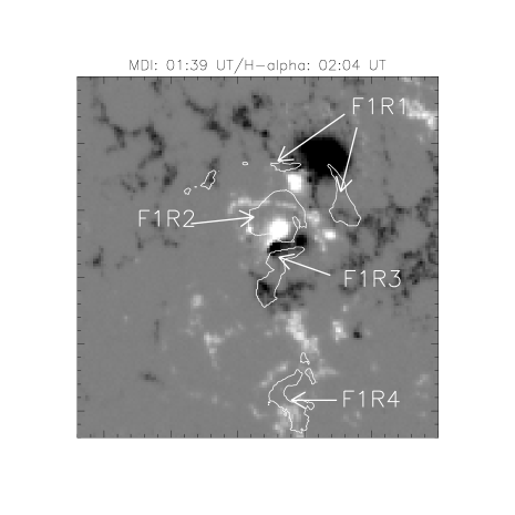
Figure 7.: Location of the M1.4 (a) and M9.6 (b) flare ribbons on the closest in time MDI magnetogram. The field of view of the images is the same as in Figure 4.

3.2.2 Nonthermal Emission

Around 01:50 UT, during the M1.4 flare peak in soft X-rays (Figure 1), RHESSI observed three non-thermal sources in the 20-60 keV energy band (Figure 6). The northern and the eastern sources were located close to the H$\alpha$ ribbons F1R1 and F1R2, respectively, while the third source might have been a signature of reconnection in the corona, located above newly reconnected loops connecting F1R1 and F1R2. The magnetic topology study presented in Section 4.1 supports this interpretation. Unfortunately, we could not produce RHESSI images at other times during the flare, due to the low count rate.

Comparing the hard X-ray footpoint sources with the photospheric magnetic field (Figure 6b), one can see that the stronger (eastern) source is located in a region of weak field, whereas the weaker (northern) source is located in the strong sunspot field. Such an asymmetry was initially reported by Sakao94, who interpreted it as a magnetic mirroring effect. That is, a weaker field at a footpoint permits a higher electron precipitation rate than a stronger field. This suggestion was later confirmed by several authors (Kundu95; Li97; Aschwanden99b; see also Cristiani et al. (2008, 2009) , for similar results in the case of submillimeter observations), and it applies to this studied event too.

3.2.3 Filament Dynamic Evolution and CME

As mentioned in Section 2.1, the M1.4 flare was accompanied by a CME. The CME was rather slow ($\approx$ 364 km s^-1) and had a low angular width ($\approx$60^∘). It became visible in the Large Angle and Spectrometric Coronagraph (LASCO, Brueckner95) C2 field of view at 02:48 UT (see http://cdaw.gsfc.nasa.gov/CME˙list/). Extrapolating back the LASCO height-time plot yields an approximate start time of the CME at about 01:40 UT, consistent with the time of the pre-flare phase.

Two elongated filaments were present at the east of the AR. They displayed a very dynamic behaviour around the time of the flare; however, they did not participate in the eruption. During the pre-flare phase, their central sections approached each other; while during the main flare phase, they seemed to merge, and shortly after they disconnected again, having different footpoint connections (Figure 5; see also Kumar09).

These two filaments were located above two PILs, which we observed to shift closer to each other during the rotation of the negative polarity N2^′ around P2 (see Section 3.1). The motion and dispersion of the negative polarities (N2^′ and smaller ones) is likely to be at the origin of the approach of the two H$\alpha$ filaments. As the positive magnetic flux between the filaments (marked P0 in the top left panel of Figure 2) became too weak, independent magnetic configurations are no longer possible. As a result, the magnetic configuration reconnects and the filaments merge to form a new configuration. After the flare, the two filaments are still present, but display a different pattern: a $\cup$-shaped filament lies at the north of a $\cap$-shaped one (Figure 5d).

In the view of Kumar09, the flare was triggered by the interaction of the two filaments. In our view there was no direct cause-and-effect between the interaction of the filaments and the flare, since none of the flare signatures observed in the available wavelengths was located close to or magnetically connected to the merging point of the filaments (see Section 4). The merging of the filaments is expected to involve magnetic reconnection as proposed by Kumar09; however, this reconnection apparently releases much less energy than the reconnection involved in the flare. Therefore, we believe that both the dynamic behaviour of the filaments and the flare were rather independent signatures of a large-scale dynamic reconfiguration of the AR field, as a result of the continuous stressing of the field by the emerging and rotating bipole in its center (see Section 3.1). A numerical simulation of the interaction of these filaments is presented in torok10.

           

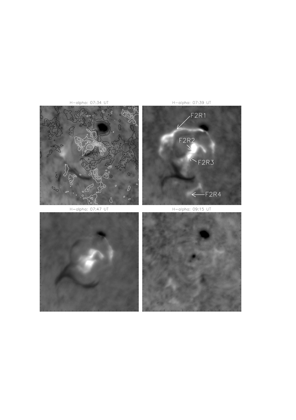
Figure 8.: Evolution of M9.6 flare in H$\alpha$. The flare ribbons are marked by F2R1, F2R2, F2R3 and F2R4, respectively. In panel (a) the contours of magnetic field (06:27 UT) are overploted (white: positive, black: negative polarity, contour level: $\pm$100, $\pm$500 G). The FOV of images is same as in Figure 4.

3.3 The M9.6 Class Flare

3.3.1 Chromospheric Evolution

The M9.6 flare was preceded by a C3.8 event that also took place in AR 10501 (see Figure 1). Due to a data gap in our H$\alpha$ observations between 07:21 UT and 07:34 UT, we could not locate the brightenings related to this event. The H$\alpha$ evolution of the M9.6 flare is shown in Figure 8, where the different ribbons are denoted as F2R1, F2R2, F2R3 and F2R4, respectively. The first H$\alpha$ emission started at $\approx$ 07:35 UT in the eastern section of F2R1 and propagated towards the western section of the ribbon. The two central ribbons, F2R2 and F2R3, became clearly visible and well-defined $\approx$ 2 minutes later. At that time F2R4 became visible too. The two central ribbons clearly separated with time, as typically seen in two-ribbon flares. The emission in these ribbons was more intense and lasted longer than in the outer ribbons (F2R1 and F2R4). The presence of a strong shear in the field could be inferred from the locations of F2R2 and F2R3 at both sides of the PIL; F2R2 was located significantly more to the north-west than F2R3 (see Figures 7 and 8), implying that the magnetic helicity was negative in that region. This is consistent with the sign of the helicity injected into the region by the clockwise rotation of N2^′ around P2 in the central bipole of the AR (Section 3.1; see also Figures 2 and 3).

In Figure 7, we show the locations of the ribbons for both flares. It can be seen that there are four ribbons in both events and that they are located at almost the same positions, i.e., the flares were morphologically very similar. Ribbon F1R1 appears to be split in several bright parts in Figure 7, but it can be seen in Figure 5 that it was in fact continuous. F2R2 and F2R3 are somewhat more compact than F1R2 and F1R3, and F2R4 is shifted and rotated in the clockwise direction compared to F1R4. A comparison of the intensities reveals that, overall, the ribbons were brighter in the M9.6 event.

Due to seeing limitations and the limited resolution of the H$\alpha$ observations, it was sometimes difficult to clearly follow the evolution of the flare ribbons. Still, we could observe an interesting difference between the two events. Although the ribbons were morphologically similar and located at almost the same places in the AR, the temporal evolution of their emission was different: during the first flare, the central ribbons, F1R2 and F1R3, appeared before the outer ones (see Section 3.2), while for the second flare, the northern ribbons F2R1 and F2R2 appeared before the southern ones.

The temporal evolution of the flare brightenings and the northern ribbons appearence (see Section 4.3), leads us to conclude that a so-called lateral breakout mechanism is the most plausible scenario for the initiation of the second event. Similar observational characteristics have been found in other events (see, e.g., Aulanier00; Gary04; Harra05; Williams05; Mandrini06).

3.3.2 Filament Eruption and Associated CME

After the first flare, the two elongated filaments with their central parts, initially orientated along north-south direction, change their orientation to an east-west direction (see Section 3.2.3). As time progresses, the filaments slowly separate from each other. Around 07:35 UT, the northern filament became partly unstable and its southern section moved quickly towards the southern filament. The two filaments then interacted, forming a structure with the shape of the letter “Y” (Figure 8). The shape of this structure and its temporal evolution indicate that the northern and the southern filaments were merging (see the H$\alpha$ movie, ar10501-halpha.mpg). Moreover, flare ribbons were developing during this evolution. Therefore, this reconfiguration can be interpreted as being due to magnetic reconnection between the magnetic configurations of the two filaments.

Next, between 7:55 and 8:04 UT, the northern filament split in two parts (see the H$\alpha$ movie). One part stayed mostly in place, while the other part erupted. These two parts probably correspond to the low and high sections of a partial filament eruption, respectively Gibson and Fan (2006). Flare ribbons were present, so magnetic reconnection was involved in the eruption. The erupting filament material could be seen moving south-west to a location in between F2R2 and F2R3 and disappeared afterwards from the H$\alpha$ images. This eruption is interpreted as being due to the reconnection of the magnetic arcade overlying the northern filament with the arcade overlying the southern filament. This filament eruption was probably associated with a full halo CME that became visible in LASCO/C2 at 08:26 UT. This CME was faster ($\approx$ 670 km s^-1) than the one associated with the first flare.

The southern filament was still visible at 08:39 UT in H$\alpha$, i.e., it was probably not involved in the CME. However, it seems that later on it erupted as well and did not reappear, at least as far as our H$\alpha$ data extend (see Figure 8d and the accompanying H$\alpha$ movie). Much later, after 11:30 UT, the formation of a large-scale arcade was observed at the south of the AR by EIT in 195 Å. It was probably the signature of reconnection occuring well behind the CME, involving the formation of closed loops (due to relaxation of the magnetic field).

4 The Magnetic Field Topology

4.1 Magnetic Field Model

The computation of the magnetic field connectivity and of its evolution is relevant to understand the homologous characteristics of the two M-class flares. Furthermore, the combination of the analysis of their temporal and spatial evolution with the computation of the magnetic field topology in the AR sets constrains on the energy release mechanisms and the initiation processes of the studied events (see Sections 3.2 and 3.3).

The line of sight magnetic field of AR 10501 is extrapolated to the corona using the discrete fast Fourier transform method under the linear force-free field (LFFF) hypothesis (${\mathbf{\nabla}}\times{\mathbf{B}}=\alpha{\mathbf{B}}$, where ${\mathbf{B}}$ is the magnetic field and $\alpha$ is a constant related to the intensity of the coronal electric currents). The method and its limitations are discussed in Demoulin97.

As boundary condition for the coronal magnetic model, we use the MDI magnetogram closest in time to each flare onset (at 03:15 UT for the first flare and at 07:59 UT for the second flare). For each magnetogram, we use a range of $\alpha$ values to compute different magnetic field models. For this particular study, the value of the free parameter of each model, $\alpha$, is chosen such that the ribbons observed during the flare main phases can be connected in pairs. We have chosen this approach since no EUV or soft X-ray images, in which coronal loops would have been clearly visible, were available for times close to the studied events.

Chandra10 analyzed the magnetic field connectivity and computed the magnetic helicity injection in AR 10501 in search for an explanation of the link between the flares and CMEs, that occurred on 18 November 2003, and the interplanetary magnetic cloud observed at 1 AU on 20 November. The aim of that study was to understand why an AR that had a global negative magnetic helicity could expel a positive helicity magnetic cloud to the interplanetary medium. These authors found that a single $\alpha$ value was not sufficient to represent the connectivity between different polarities in the AR. The observed loops in some regions of the AR could be modeled using a negative $\alpha$ value, while a positive $\alpha$ value was needed for others. The computed maps of the magnetic helicity flux density also showed mixed helicity signs. Furthermore, there was observational evidence of different chiralities in different sections of the filaments seen in H$\alpha$. It was finally concluded that positive magnetic helicity had been injected into a connectivity domain at the south of the AR. The CME and associated magnetic cloud were ejected from this region.

The mixed helicity sign pattern just described seems to be present also in the AR configuration on 20 November. Different sections of the observed H$\alpha$ ribbons can be connected in pairs using $\alpha$ values ranging from negative to positive values. In all cases, the value of $\alpha$ is low, between $-9.4\times$10^-3Mm^-1 and $7.5\times$ 10^-3Mm^-1. We will discuss the magnetic field connectivity and its implications for the flare initiation process in Section 4.2, after briefly introducing the definition of QSLs and the method used to compute their locations.

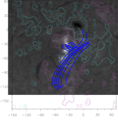
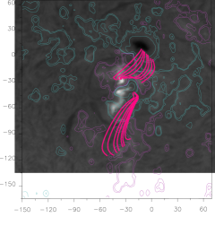
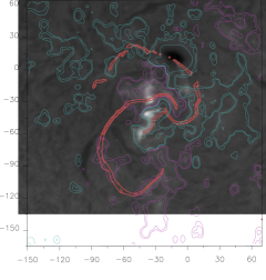
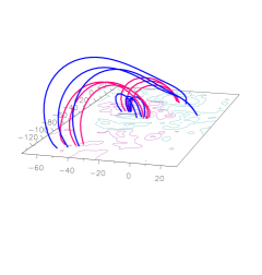
Figure 9.: (a,b): H$\alpha$ image of the first flare at 02:17 UT overlaid by magnetic field lines computed from either side of the photospheric traces of the QSLs shown in (c). (c): Intersection of the QSLs with the photospheric plane computed from the MDI magnetogram at 03:15 UT, overlaid on the H$\alpha$ image. Panels (a-c) are drawn in the observer’s point of view. (d): Perspective view of the field lines shown in panels (a) and (b). The field lines have been selected to illustrate the coronal linkage at the edges of QSLs. The field of view is a portion of the one shown in (a-c). Field lines drawn in blue (red) represent loops before (after) reconnection at a QSL, as inferred from the analysis of the flare evolution (see Section 4.3). All panels correspond to the magnetic field model with the lowest (negative) $\alpha$ value. The negative and positive magnetic field contour levels ($\pm$ 50, 100, 500 gauss (G) in (a–c), and $\pm$ 100, 500 G in (d)) are represented in cyan and pink colours, respectively.

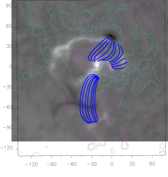
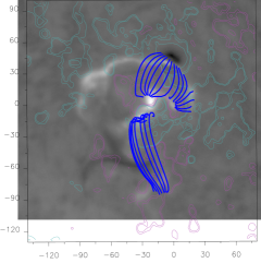
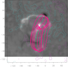
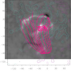
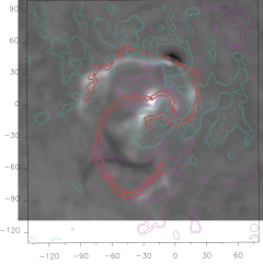
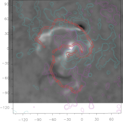
Figure 10.: (a-d): H$\alpha$ image of the second flare at 07:39 UT overlaid by magnetic field lines computed from either side, or close to, the photospheric traces of QSLs shown in (e) and (f). (e,f): Intersection of the QSLs with the photospheric plane, computed from the MDI magnetogram at 07:59 UT overlaid on the H$\alpha$ image at 07:39 UT. The panels in the left column correspond to the magnetic field model using the lowest (negative) $\alpha$ value (with some field lines computed from a potential field model added), the panels in the right column correspond to the model using the highest (positive) value for $\alpha$. Field lines drawn with continuous blue (red) lines represent loops before (after) reconnection at a QSL, as inferred from the analysis of the flare evolution (see Section 4.3). The negative and positive magnetic field contour levels ($\pm$ 50, 100, 500 G) are shown in cyan and pink colours, respectively. All panels have been drawn in the observer’s point of view.

4.2 QSLs Locations and Flare Ribbons

QSLs are defined as regions where there is a drastic change in field line connectivity, as opposed to the extreme case of separatrices where the connectivity is discontinuous (see references in Section 1). The location of QSLs can be determined by computing the squashing degree $Q$ Titov, Hornig, and Démoulin (2002). A QSL is defined where $Q\gg 2$ (the value $Q=2$ is the lowest possible one). The squashing degree increases where connectivity gradients grow, and it becomes infinitely large where the field line mapping becomes discontinuous, i.e., for separatrices. By definition, $Q$ is uniquely defined along a field line by $({\mathbf{B}}\cdot{\mathbf{\nabla}})Q=0$.

The numerical procedure used to determine the values of $Q$ has been thoroughly discussed by Aulanier05. The magnetic field model used here takes observed magnetograms as the boundary condition. Therefore, the presence of parasitic polarities results in multiple QSLs. However, we only show those corresponding to the highest values of $Q$ ($\log_{10}Q$ above $\approx 6$). In other words, only the thinnest QSLs, those where thin electric current sheets favourable for reconnection are most likely to build up, are shown in Figures 9 and 10. It is worth noting that, in all our computations of the coronal magnetic field, no magnetic null points were found that could be related to the large scale connections between the flare ribbons, i.e. there are no separatrices which can explain the location of the observed H$\alpha$ ribbons.

Figures 9 and 10 show the intersections of the QSLs with the photospheric plane, together with the locations of H$\alpha$ ribbons at times corresponding to the main phases of the M1.4 and M9.6 flares, respectively. The linkage of the coronal magnetic field is outlined by field lines having footpoints on either side, and close to, the photospheric traces of the QSLs.

Two elongated QSLs are present in the AR configuration, as has been found in cases analyzed previously (Demoulin97; Mandrini97). The flare ribbons for both events are located at, or close to, the photospheric QSL traces. For the first flare, we only show the results for a magnetic field model with $\alpha$ = -9.4 $\times$10^-3Mm^-1 (Figure 9), while for the second flare we show the results for both values of $\alpha$, -9.4 $\times$10^-3Mm^-1 and 7.5 $\times$ 10^-3Mm^-1 (Figure 10). The different sets of field lines drawn in these figures illustrate the main connectivity domains in AR 10501. We have also added some field lines computed using a potential field model in Figures 10a and c, since the linkage between the ribbons is better represented by them along some sections of the QSLs. In what follows we discuss the results for the M9.6 flare. The same results are valid for the M1.4 event.

For the second flare, one set of field lines connects flare ribbons F2R1 to F2R2, a second set F2R2 to F2R3, a third set F2R3 to F2R4, and a fourth set F2R1 to F2R4 (see Figure 10). As discussed in Section 4.1, our choice of $\alpha$ was done such that the flare ribbons could be connected by field lines in pairs. Using either a negative or positive $\alpha$ value, ribbons F2R2 and F2R3 overlap very well with photospheric QSL traces along all their extensions (Figures 10). The same is true for the western part of F2R1. Its eastern part, however, does not overlap that well with the QSL trace, most probably because the QSL is broad there (lower $Q$ values). Therefore, its location is more sensible to the coronal current distribution. Finally, ribbon F2R4 is located closer to a QSL trace in the model with negative $\alpha$.

A linear force-free model implies that $\alpha$ is constant in the whole AR. However, from our previous discussion (Section 4.1), we can assume that this is not the case for AR 10501, since it seemed to retain the same mixed helicity pattern found on 18 November Chandra et al. (2010). Therefore, the partial lack of coincidence between the spatial locations of QSLs and flare ribbons comes most probably from the intrinsic limitations of our modelling. In spite of this, there is a global agreement between the QSL traces and flare ribbons for both events (Figures 9 and 10). Furthermore, these traces are similar even though QSLs have been computed using two different magnetograms as boundary conditions (at 03:15UT and at 07:59 UT); this means that the magnetic configuration involved in both flares remained approximately the same, explaining the homology between them.

In addition, we found that for all the $\alpha$ values used, the resulting overall pattern of the QSL traces was similar. This indicates that the locations of QSLs are mainly determined by the photospheric distribution of the magnetic polarities. For both events, the flare ribbons can be connected in pairs by field lines whose foopoints lie on both sides of a QSL (Figures 9 and 10). We therefore conclude that magnetic reconnection at QSLs is at the origin of both homologous flares.

4.3 Physical Scenario of the Eruptive Flares

The comparison of the observed flare ribbons and the photospheric trace of QSLs shows that reconnection at QSLs is involved in the flares, but it does not explain which are the reconnected field lines, since the spatial comparison is not precise enough to tell on which side of a QSL is a given ribbon, i.e., if reconnected field lines are connecting the inner (resp. the outer) pair of ribbons or if they are connecting the northern (resp. southern) pair of ribbons. However, there are several observational clues to determine the connectivities after reconnection. A classical one is to observe flare loops in UV or/and in H$\alpha$. Unfortunately, in the analyzed observations, there is no clear evidence of flare loops. A related clue is the observation of hard X-rays sources at the footpoints or/and near the top of reconnected loops. Those are observed during the first flare (Figure 6b). Another clue is the increasing separation with time of a pair of ribbons located at both sides of a PIL, as observed in the second flare.

The main evidence for the field connections after reconnection in the M1.4 flare are the spatial locations of the three hard X-rays sources observed by RHESSI (Figure 6b). They imply that reconnected field lines connect F1R1 to F1R2 and, by inference, also F1R3 to F1R4 (drawn with red lines in Figures 9b and d). There are no detectable hard X-ray sources, and the H$\alpha$ ribbons are weaker, for these southern connections, most probably because the magnetic configuration is very asymmetric in magnetic field strength, so that there is only a low energy input into the southern reconnected loops. The new connections (F1R1 to F1R2, F1R3 to F1R4) are each located above an H$\alpha$ filament. It can be assumed that the downward magnetic field tension of these new connections increases the stability of the magnetic configurations of the filaments. Indeed, these two filaments were staying unperturbed during and after the M1.4 flare. Finally, we infer from the above observational facts that the connections before reconnection are field lines connecting F1R2 to F1R3 and F1R1 to F1R4 (drawn with blue lines in Figures 9a and d). This conclusion is coherent with the strong shearing motion observed in between F1R2 and F1R3; such a motion is likely to store magnetic energy and to expand short connections, forcing them to reconnect with the overlying large connections, as in the MB model. Recalling that we have also found evidence of the TC model in the pre-flare stage (Figure 4), we conclude that the physical mechanism at work during the eruption is first TC, followed by an MB-like mechanism.

While the flare ribbons have nearly the same locations in the M9.6 flare as in the previous flare, we found evidence that reconnection proceeded in the opposite way, as follows. For the M9.6 flare, the central ribbons clearly separated with time, indicating that new magnetic connections were formed between F2R2 and F2R3 (see the H$\alpha$ movie in the interval 7:40-8:00 UT). Moreover, between 7:55 and 8:04 UT, a part of the northern filament erupted (see Section 3.3.2). We interprete this eruption as being due to the reconnection of the magnetic arcade overlying this part of the filament (i.e., the one between F2R1 and F2R2) with the southern arcade (the one between F2R3 and F2R4; see Figure 10). Below the southern arcade, the filament was also destabilized, but later on (after 8:10 UT). We conclude that, in the M9.6 flare, the overlying arcade connecting F2R1 to F2R2 reconnected with the arcade connecting F2R3 to F2R4, i.e., in the reverse direction than in the MB model (see Section 1). This is sometimes referred to as “lateral breakout” (see the references in Sect. 3.3.1).

Although the flares are homologous, we conclude that reconnection proceeded in opposite directions for the M1.4 and M9.6 flares. Reconnection occurring successively in a reverse direction during a a flare has been also reported by Goff07 and by Karpen98 as result of an MHD simulation. However, in the flare studied by Goff07, the reconnection took place in successive phases of the same flare and the reversal of the reconnection direction in the last phase was interpreted as a “bouncing back” due to a too strong forcing in the previous eruptive phase. In the homologous flares studied here, the reversal has another origin, as we discuss below.

First, the strong shearing induced by the motion of N2^′ (and by other smaller negative polarities) leads to the expansion of the field lines connecting P2 to N2^′. There is also diffusion of the magnetic field towards the PIL, which is accompanied by flux cancelation and, most probably, by the build up of a flux rope, as in the MHD simulation of Aulanier10. The pre-flare brightenings (Figure 4) are a trace of this slow reconnection process. Then, at some point of the evolution, either a fast quadrupolar reconnection process starts or the flux rope becomes unstable and the M1.4 flare occurs. Since the motion of N2^′ continues (Figure 3), we could expect that a similar flare, with the same reconnection direction, would occur later on. However the build-up of magnetic stress is occurring also along other PILs of the AR, since there is a large photospheric dispersion of the magnetic field from the main spot (see the MDI movie). As described above, converging flows are increasing the magnetic shear, force flux cancelation, and probably also build a flux rope. This process is especially active in between P1, P2, and the eastern diffuse negative polarity (both large flows and a large amount of magnetic flux are involved). We suggest that this process was strong enough to build up a too stressed, hence unstable, field configuration at the location of the northern filament, (i.e., between F2R1 and F2R2), inducing the M9.6 flare. Therefore, since the eruption starts in a connectivity domain different from that of the first flare, the successive reconnections proceed in the opposite order in the two flares.

5 Conclusions

We studied two homologous flares on 20 November 2003 that occurred in AR 10501. The active region is characterized by multiple polarities and by a significant rotation ($\approx 110^{\circ}$) of a negative polarity around the corresponding positive polarity of an emerging bipole. This continuous rotation supplies free energy to the active region. The AR is also characterized by a large diffusion of the magnetic flux from a main sunspot (polarity N1), accompanied by the convergence and subsequent cancellation of opposite polarities at the photospheric inversion lines (PILs). This process also increases the stress of the coronal magnetic field.

Four flare ribbons are observed in each flare, indicating that reconnection occurs in a quadrupolar configuration. The photospheric magnetic field was extrapolated, using the linear, or constant $\alpha$, force-free-field approximation. Due to the complexity of the AR, in particular, evidence of magnetic helicity with mixed signs two days before, we computed the QSL locations using positive as well as negative $\alpha$ values. In agreement with previous studies (see references in Section 1), the H$\alpha$ flare ribbons are found in the vicinity of the photospheric trace of QSLs. They are magnetically linked in pairs, as expected for a quadrupolar configuration. Since the large-scale connections of the coronal field are only weakly sheared, the photospheric traces of QSLs are located at almost the same positions for cases with $\alpha<0$ and $>0$. Thus, the QSL locations are mainly determined by the spatial distribution of the photospheric polarities, and to a much lesser extent by the coronal currents. However, we found that $\alpha$ values of different sign are required to model the magnetic connection between different pairs of ribbons, which supports the presence of mixed helicity in the AR.

Thanks to the high time cadence of the H$\alpha$ observations, we also observed the fast drift of the emission along one ribbon (F2R1). This can be interpreted as a slip-running magnetic reconnection process Aulanier et al. (2007), which is a characteristic of reconnection at QSLs with finite thickness (in contrast to an instantaneous change of connectivity for reconnection across separatrices).

The location of the pre-flare brightenings suggests that the first flare was initiated by “tether cutting” at the central PIL. A significant motion of a nearby magnetic polarity was observed for about 8 hours before the flare, providing a very sheared core field, in agreement with vector magnetogram observations. Later on, this core field erupted, accompanied by the formation of a four-ribbon flare. Tether cutting reconnection at the PIL, i.e., the transformation of a sheared arcade into a flux rope, appears to be the mechanism starting the eruption. Subsequent quadrupolar reconnection is evident from the observed pattern of the flare ribbons; this presumably destabilized the configuration even more (as in the magnetic breakout model). The flux rope eruption itself may have been driven by an instability or catastrophic loss of equilibrium. Present observations are not sufficient to separate the respective roles of these mechanisms.

The second flare had a very similar spatial organization of the H$\alpha$ ribbons, i.e., it was homologous to the first one. However, we found observational evidence that magnetic reconnection occurs in a direction reverse to that of the first flare (e.g., the pieces of evidence are the evolution of the ribbon separation from the central PIL and the locations where the filaments erupt, below the lateral field connections of the quadrupolar configuration). This is surprising at first, since the observed shearing motions continued well after the time of the flares. However, there was also a significant diffusion of the magnetic field around the main sunspot, especially in the northern part of the AR. This leads to converging motions and magnetic cancelation along the nearby PIL, as well as to an increase of the magnetic shear. We conclude that the second flare occurred as this process destabilized the northern lateral connectivity domain of the quadrupolar configuration, i.e., the second eruption started in a different domain than the first one. This resulted in a flare with similar ribbons, but with a reconnection direction opposite to the one during the first flare.

More generally, we suggest that in a complex magnetic configuration with several connectivity domains (separated by separatrices or QSLs), horizontal motions of the polarities, magnetic diffusion toward the PILs, as well as newly emerging flux, will all compete in increasing the local stress of each connectivity region. Depending on the relative importance of these processes, but also on the previous history (like the launch of a CME from one of the connectivity domain), the stressed magnetic field of one of the connectivity domains will become the next unstable region. As long as the photospheric flux distribution is not drastically changed, the successive flares will be homologous, i.e., they will display the same global pattern of flare ribbons. This is because, for multipolar fields, QSL locations are determined mainly by the global organization of the photospheric polarities and QSLs are structurally stable (while separatrices can appear or disappear after a bifurcation of the topology). In the absence of significant emergence, the only possible change expected from one flare to the next is the location of the next unstable connectivity domain, i.e., the location where the next unstable pre-CME core field is forming.

Acknowledgements

R.C. thanks Centre Franco-Indien pour la Promotion de la Recherche Avancée (CEFIPRA) for his postdoctoral grant. C.H.M. thanks the Argentinean grants: UBACyT X127 and PICT 2007-1790 (ANPCyT). C.H.M. is a member of the Carrera del Investigador Científico, CONICET. The research leading to these results has received funding from the European Commission’s Seventh Framework Programme (FP7/2007-2013) under the grant agreement n^o 218816 (SOTERIA project, www.soteria-space.eu). Financial support by the European Comission through the SOLAIRE network (MTRM-CT-2006-035484) is also gratefully acknowledged. We acknowledge the use of TRACE data. MDI data are a courtesy of SOHO/MDI consortium. SOHO is a project of international cooperation between ESA and NASA. B.S, C.H.M, RC have started and discussed this work in the frame of the ISSI workshop chaired by Dr. Consuelo Cid (2008-2010). The authors acknowledge financial support from ECOS-Sud (France)/MINCyT (Argentina) through their cooperative science program (N^o A08U01). We also thank the anonymous referee’s constructive comments and suggestions.

References

- Antiochos (1998) Antiochos, S.K.: 1998, ApJ 502, 181.
- Antiochos, DeVore, and Klimchuk (1999) Antiochos, S.K., DeVore, C.R., Klimchuk, J.A.: 1999, ApJ 510, 485.
- Aschwanden et al. (1999) Aschwanden, M.J., Fletcher, L., Sakao, T., Kosugi, T., Hudson, H.: 1999, ApJ 517, 977.
- Aulanier et al. (2000) Aulanier, G., DeLuca, E.E., Antiochos, S.K., McMullen, R.A., Golub, L.: 2000, ApJ 540, 1126.
- Aulanier et al. (2007) Aulanier, G., Golub, L., DeLuca, E.E., Cirtain, J.W., Kano, R., Lundquist, L.L., Narukage, N., Sakao, T., Weber, M.A.: 2007, Science 318, 1588.
- Aulanier, Pariat, and Démoulin (2005) Aulanier, G., Pariat, E., Démoulin, P.: 2005, A&A 444, 961.
- Aulanier et al. (2006) Aulanier, G., Pariat, E., Démoulin, P., Devore, C.R.: 2006,Sol. Phys. 238, 347.
- Aulanier et al. (2010) Aulanier, G., Török, T., Démoulin, P., DeLuca, E.E.: 2010,ApJ 708, 314.
- Bagalá et al. (2000) Bagalá, L.G., Mandrini, C.H., Rovira, M.G., Démoulin, P.: 2000, A&A 363, 779.
- Bleybel et al. (2002) Bleybel, A., Amari, T., van Driel-Gesztelyi, L., Leka, K.D.: 2002, A&A 395, 685.
- Brueckner et al. (1995) Brueckner, G.E., Howard, R.A., Koomen, M.J., Korendyke, C.M., Michels, D.J., Moses, J.D., et al.: 1995,Sol. Phys. 162, 357.
- Carmichael (1964) Carmichael H.: 1964, In: Hess, W.N. (ed.), The Physics of Solar Flares, NASA SP-50, 451.
- Chandra et al. (2010) Chandra, R., Pariat, E., Schmieder, B., Mandrini, C.H., Uddin, W.: 2010, Sol. Phys. 261, 127.
- Cristiani et al. (2009) Cristiani, G., Giménez de Castro, C.G., Mandrini, C.H., Machado, M.E., Rovira, M.G.: 2009, Adv. Space. Res. 44, 1314.
- Cristiani et al. (2008) Cristiani, G., Giménez de Castro, C.G., Mandrini, C.H., Machado, M.E., Silva, I.D.B.E., Kaufmann, P., Rovira, M.G.: 2008, A&A 492, 215.
- Démoulin (2007) Démoulin, P.: 2007, Adv. Space. Res. 39, 1367.
- Démoulin et al. (1997) Démoulin, P., Bagala, L.G., Mandrini, C.H., Henoux, J.C., Rovira, M.G.: 1997, A&A 325, 305.
- Démoulin et al. (1996) Démoulin, P., Hénoux, J.C., Priest, E.R., Mandrini, C.H.: 1996, A&A 308, 643.
- Démoulin, Priest, and Lonie (1996) Démoulin, P., Priest, E.R., Lonie, D.P.: 1996, J. Geophys. Res. 101, 7631.
- DeVore and Antiochos (2008) DeVore, C.R., Antiochos, S.K.: 2008, ApJ 680, 740.
- Forbes (2000) Forbes, T.G.: 2000, J. Geophys. Res. 105, 23153.
- Forbes and Isenberg (1991) Forbes, T.G., Isenberg, P.A.: 1991, ApJ 373, 294.
- Gary and Moore (2004) Gary, G.A., Moore, R.L.: 2004, ApJ 611, 545.
- Gibson and Fan (2006) Gibson, S.E., Fan, Y.: 2006, ApJ 637, 65.
- Goff et al. (2007) Goff, C.P., van Driel-Gesztelyi, L., Démoulin, P., Culhane, J.L., Matthews, S.A., Harra, L.K., Mandrini, C.H., Klein, K.L., Kurokawa, H.: 2007, Sol. Phys. 240, 283.
- Gopalswamy et al. (2005) Gopalswamy, N., Yashiro, S., Michalek, G., Xie, H., Lepping, R.P., Howard, R.A.: 2005, Geophys. Res. Lett. 32, 12.
- Harra et al. (2005) Harra, L.K., Démoulin, P., Mandrini, C.H., Matthews, S.A., van Driel-Gesztelyi, L., Culhane, J.L., Fletcher, L.: 2005, A&A 438, 1099.
- Hirayama (1974) Hirayama, T.: 1974, Sol. Phys. 34, 323.
- Hurford et al. (2002) Hurford, G.J., Schmahl, E.J., Schwartz, R.A., Conway, A.J., Aschwanden, M.J., Csillaghy, A., et al.: 2002, Sol. Phys. 210, 61.
- Karpen et al. (1998) Karpen, J.T., Antiochos, S.K., Devore, C.R., Golub, L.: 1998, ApJ 495, 491.
- Kliem and Török (2006) Kliem, B., Török, T.: 2006, Phys. Rev. Lett. 96, 255002.
- Kopp and Pneuman (1976) Kopp, R.A., Pneuman, G.W.: 1976, Sol. Phys. 50, 85.
- Kumar, Manoharan, and Uddin (2010) Kumar, P., Manoharan, P.K., Uddin, W.: 2010, ApJ 710, 1195.
- Kundu et al. (1995) Kundu, M.R., Nitta, N., White, S.M., Shibasaki, K., Enome, S., Sakao, T., Kosugi, T., Sakurai, T.: 1995, ApJ 454, 522.
- Li et al. (1997) Li, J., Metcalf, T.R., Canfield, R.C., Wuelser, J., Kosugi, T.: 1997, ApJ 482, 490.
- Lin et al. (2002) Lin, R.P., Dennis, B.R., Hurford, G.J., Smith, D.M., Zehnder, A., Harvey, P.R., et al.: 2002, Sol. Phys. 210, 3.
- Machado (1985) Machado, M.E.: 1985, Sol. Phys. 99, 159.
- Machado et al. (1988) Machado, M.E., Moore, R.L., Hernandez, A.M., Rovira, M.G., Hagyard, M.J., Smith, J.B. Jr.: 1988, ApJ 326, 425.
- MacTaggart and Hood (2009) MacTaggart, D., Hood, A.W.: 2009, A&A 508, 445.
- Mandrini (2010) Mandrini C.H.: 2010, In: Kosovichev, A. G., Andrei, A. H., Roelot, J. P. (eds.), Solar and Stellar Variability: Impact on Earth and Planets, IAU Symp. 264, 257.
- Mandrini et al. (1997) Mandrini, C.H., Démoulin, P., Bagala, L.G., van Driel-Gesztelyi, L., Henoux, J.C., Schmieder, B., Rovira, M.G.: 1997, Sol. Phys. 174, 229.
- Mandrini et al. (1991) Mandrini, C.H., Démoulin, P., Henoux, J.C., Machado, M.E.: 1991, A&A 250, 541.
- Mandrini et al. (2006) Mandrini, C.H., Démoulin, P., Schmieder, B., Deluca, E.E., Pariat, E., Uddin, W.: 2006, Sol. Phys. 238, 293.
- Martres (1989) Martres, M.J.: 1989, Sol. Phys. 119, 357.
- Masson et al. (2009) Masson, S., Pariat, E., Aulanier, G., Schrijver, C.J.: 2009, ApJ 700, 559.
- Moore and Roumeliotis (1992) Moore R.L., Roumeliotis G.: 1992, In: Svestka, Z., Jackson, B. V., Machado, M. E. (eds.), Eruptive Solar Flares, IAU Colloq. 133, 69.
- Moore and Sterling (2006) Moore, R.L., Sterling, A.C.: 2006, In: Gopalswamy, N., Mewaldt, R., Torsti, J. (eds.), Solar Eruptions and Energetic Particles, AGU Geophysical Monograph 165, 43.
- Moore et al. (2001) Moore, R.L., Sterling, A.C., Hudson, H.S., Lemen, J.R.: 2001, ApJ 552, 833.
- Möstl et al. (2008) Möstl, C., Miklenic, C., Farrugia, C.J., Temmer, M., Veronig, A., Galvin, A.B., Vrsnak, B., Biernat, H.K.: 2008, Ann. Geophys 26, 3139.
- Priest and Démoulin (1995) Priest, E.R., Démoulin, P.: 1995, J. Geophys. Res. 100, 23443.
- Ranns et al. (2000) Ranns, N.D.R., Matthews, S.A., Harra, L.K., Culhane, J.L.: 2000, A&A 364, 859.
- Sakao (1994) Sakao T.: 1994, ‘Characteristics of Solar Flares Hard X-ray Sources as Revealed with the Hard X-ray Telescope aboard the Yohkoh Satellite’, Ph.D. thesis, University of Tokyo.
- Scherrer et al. (1995) Scherrer, P.H., Bogart, R.S., Bush, R.I., Hoeksema, J.T., Kosovichev, A.G., Schou, J., et al.: 1995, Sol. Phys. 162, 129.
- Schrijver (2009) Schrijver, C.J.: 2009, Adv. Space. Res. 43, 739.
- Srivastava et al. (2009) Srivastava, N., Mathew, S.K., Louis, R.E., Wiegelmann, T.: 2009, J. Geophys. Res. 114, 3107.
- Sterling and Moore (2001) Sterling, A.C., Moore, R.L.: 2001, J. Geophys. Res. 106, 25227.
- Sturrock (1966) Sturrock, P.A.: 1966, Nature 211, 695.
- Takasaki et al. (2004) Takasaki, H., Asai, A., Kiyohara, J., Shimojo, M., Terasawa, T., Takei, Y., Shibata, K.: 2004, ApJ 613, 592.
- Titov, Hornig, and Démoulin (2002) Titov, V.S., Hornig, G., Démoulin, P.: 2002, J. Geophys. Res. 107(A8), SSH 3-1.
- Török et al. (2010) Török, T., Chandra, R., Pariat, E., Démoulin, P., Schmieder, B., Aulanier, G., Linton, M.G., Mandrini, C.H.: 2010, ApJ, submitted.
- Török and Kliem (2005) Török, T., Kliem, B.: 2005, ApJ 630, 97.
- Uddin et al. (2004) Uddin, W., Jain, R., Yoshimura, K., Chandra, R., Sakao, T., Joshi, A., Despande, M.R.: 2004, Sol. Phys. 225, 325.
- Waldmeier (1938) Waldmeier, M.: 1938, Z. Astrophys. 16, 276.
- Williams et al. (2005) Williams, D.R., Török, T., Démoulin, P., van Driel-Gesztelyi, L., Kliem, B.: 2005, ApJ 628, 163.
- Woodgate et al. (1984) Woodgate, B.E., Martres, M., Smith, J.B. Jr., Strong, K.T., McCabe, M.K., Machado, M.E., Gaisauskas, V., Stewart, R.T., Sturrock, P.A.: 1984, Adv. Space. Res. 4, 11.
- Xu et al. (2010) Xu, Y., Jing, J., Cao, W., Wang, H.: 2010, ApJ 709, 142.
- Yurchyshyn, Hu, and Abramenko (2005) Yurchyshyn, V., Hu, Q., Abramenko, V.: 2005, Space Weather 3, 8.