Correlation Widths in Quantum–Chaotic Scattering
Abstract
An important parameter to characterize the scattering matrix for quantum–chaotic scattering is the width of the –matrix autocorrelation function. We show that the “Weisskopf estimate” (where is the mean resonance spacing, with the “transmission coefficient” in channel and where the sum runs over all channels) provides a good approximation to even when the number of channels is small. That same conclusion applies also to the cross–section correlation function.
1 Purpose
Quantum–chaotic scattering is an ubiquitous phenomenon. It emerges whenever Schrödinger waves are scattered by a system with chaotic intrinsic dynamics. Examples are the passage of electrons through disordered mesoscopic samples, and compound–nucleus scattering. Moreover, it occurs when electromagnetic waves of sufficiently low frequency are transmitted through a microwave cavity with the shape of a classically chaotic billiard. In all these cases, chaotic scattering is due to the numerous quasibound states of the system that appear as resonances in the scattering process and that obey random–matrix statistics.
The generic approach to quantum–chaotic scattering [1] is based upon a random–matrix model for the resonances and, thus, for the scattering matrix , a function of energy where denote the open channels. Within that approach, the energy correlation function of the scattering matrix (the ensemble average ) can be worked out analytically [2] as a function of the energy difference , and approximate expressions for the cross–section correlation function are also available [3, 4, 5]. The correlation width of the cross section turns out to be rather close to that of the scattering matrix in all cases [5]. That is why we focus attention on the –matrix correlation function in what follows.
The analytical expression for the -matrix correlation function is given in terms of a threefold integral [2]. The numerical evaluation of that integral is quite cumbersome. To gain an orientation of what to expect in a given situation, a simple approximate expression for the width of the –matrix correlation function (and, by implication, of the cross section) would therefore be helpful. A commonly used approximation applicable in the regime of strongly overlapping resonances is the “Weisskopf estimate” [6]. It has for example been applied to resonance spectra obtained from microwave experiments on quantum chaotic scattering [5, 7]. The measurements were performed in the regimes of isolated and weakly overlapping resonances and the associated matrix comprised two dominant scattering channels and a large number of weakly coupled ones. A motivation for the present paper was to test the accuracy of the Weisskopf estimate under such conditions. We will demonstrate that it provides a good approximation for not only in the regime of strongly overlapping resonances. For simplicity and without loss of generality we confine ourselves to the case where the average –matrix is diagonal, . The unitarity deficit of the average –matrix is then measured by the transmission coefficients . These obey for all .
Naively, one might consider two alternatives for estimating . (i) The Weisskopf estimate expresses the total average resonance width in terms of the mean resonance spacing and of the transmission coefficients ,
| (1) |
The sum in Eq. (1) runs over the open channels.
(ii) The “Moldauer–Simonius sum rule” [8, 9] gives the following expression for the mean distance of the poles of the scattering matrix (labeled by a running index ) from the real energy axis.
| (2) |
For the case of unitary symmetry, the sum rule Eq. (2) has been derived rigorously [10]. There is no reason to doubt that the sum rule Eq. (2) holds also in the orthogonal case although a proof exists only in fragmentary form [11].
The width in Eq. (1) and the double average pole distance as given by Eq. (2) agree whenever for all . In general, however, the values of both quantities differ widely. For instance, for the case of a single channel with , Eq. (1) yields while Eq. (2) yields . An identification of (of ) with the correlation width would suggest that we deal with isolated (with strongly overlapping) resonances, respectively. It is known [12, 13, 14] that Eq. (2) fails when any of the is close to unity, and a comparison of the values of given in the figures below with Eq. (2) confirms that fact. We ascribe that failure of the Moldauer–Simonius sum rule to the fact that the fluctuation properties of the scattering matrix depend not only on the location of the poles of but also on the values of the residues. Little is actually known about the latter [15, 16].
That leaves us with Eq. (1) as the only viable alternative. We recall the conditions under which Eq. (1) is obtained [6]. One uses a time–dependent description and considers a scattering system with constant resonance spacing coupled to a number of channels. The frequency with which a typical wave function of the system approaches the entrance of a given channel is , the probability with which the system escapes into that channel is given by , the partial width for decay into channel is accordingly . Summing over all channels and postulating that the result applies also to systems that do not have a constant resonance spacing , one replaces by the actual mean resonance spacing and arrives at Eq. (1). The argument being semiclassical, one expects Eq. (1) to give an approximate expression for the average resonance decay width in the case of many channels or, more precisely, for .
That argument leaves open the question how relates to the correlation width . In Ericson’s work [17] the identity of and of was postulated for . A proof for that assertion became available with the work of Ref. [18]. There it was shown that an expansion of the –matrix correlation function derived in Ref. [2] in inverse powers of yields as the leading term a Lorentzian with width . This result implies in the Ericson regime of strongly overlapping resonances, i.e., for . A second case is that of many open channels each coupled weakly to the resonances. Using the analytical expression for the -matrix correlation function [2] Harney et al. [19] showed that in that case, also provides a good approximation for . Apart from these results for the regimes of strongly overlapping and of isolated resonances coupled to many channels no simple analytical expression exists for . In the present paper we investigate how much and differ for general values of the number of channels and of the coupling strength in each channel. We use the analytical result of Ref. [2] for the -matrix correlation function to compute the width numerically and compare the result with .
2 Approach
Starting point is the expression (see the review [1])
| (3) |
for the element of the scattering matrix connecting channels and , with
| (4) |
Here is the energy. The real and symmetric matrix with elements and is a member of the Gaussian orthogonal ensemble of random matrices (GOE). The elements are Gaussian–distributed random variables with zero mean values and second moments given by . The matrix represents quasibound levels and their mutual interaction. The parameter has the dimension energy and defines the average level spacing of the eigenvalues of . In the center of the GOE spectrum we have . The parameter defines the energy scale so that both and are expressed in units of . The real matrix elements couple the space of quasibound levels to channels labelled . In the cases considered in the present work the amplitudes for the passage from an intrinsic state to a scattering channel coincide with those for the reverse process, that is . Without loss of generality we assume that . The parameters define the mean strength of the coupling to channel . Since is random, the –matrix is a matrix–valued random process that depends on . All moments and correlation functions of (defined by averaging over the GOE with the energy at or close to the center of the GOE spectrum) depend only on the average –matrix elements , on the transmission coefficients , and on energy differences. The latter are expressed in units of . With we have
| (5) |
In Ref. [2], the autocorrelation and cross–correlation functions of the elements of the –matrix are given in terms of these parameters. They are worked out for fixed in the limit . We do not repeat the analytical expressions here. These contain a threefold integration over real variables. We make use of a simplification of these integrals in terms of variable transformations first introduced in Ref. [18] and summarized in the Appendix of Ref. [5]. For a given set of transmission coefficients the resulting formula for the –matrix autocorrelation function
| (6) |
is evaluated numerically as a function of . The full width at half maximum of that function yields .
3 Results
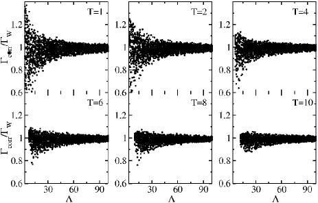
According to the Weisskopf estimate in Eq. (1), the correlation width should depend only on the number of channels and on the sum of the transmission coefficients. To test that assertion, we have for fixed values of and of with calculated the width of the autocorrelation function Eq. (6) for several sets of parameters . These are subject to the constraints and and were obtained with the help of a random–number generator. The number of sets was typically between and . We evaluated , where and take either of the channel numbers and and found that in the intermediate regime of weakly overlapping resonances, the widths of , of and of vary from set to set, in contrast to the above assertion. The deviations of the ratios from unity are of comparable size in all three cases. Therefore we show in the following only results for .
To test the dependence of on the values of associated with the incident and outgoing channels in the expression for we considered three cases. In case I, we chose arbitrarily, that is, we did not sort the transmission coefficients by size. In case II (case III) we ordered the transmission coefficients such that take the maximal values (the minimal values, respectively) of all ’s. In case II the channels and are the dominant ones, in case III they are the most weakly coupled ones. Case II is relevant for the microwave experiments described in Refs. [5, 7, 20].
In Fig. 1 we consider case I and plot for several values of given in the panels the ratio versus for the correlation function . The number of sets of chosen was . To test the statistical significance of the results we have increased the set size to and did not observe a noticeable change. Each set corresponds to a dot in the plot. The dots scatter about a mean value that is close to unity. For fixed (fixed ), the width of the cloud of dots decreases with increasing (increasing , respectively). The width indicates that in contrast to the Weisskopf formula, does depend on the values of the individual transmission coefficients. To further test this dependence we considered cases II and III. The ratios resulting from each of the 25 sets of transmission coefficients form clouds that for both cases are very narrow as compared to those shown in Fig. 1. We do not display these as they would cover the upper parts of the clouds shown in Fig. 1 in case II, the lower parts in case III.
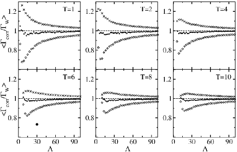
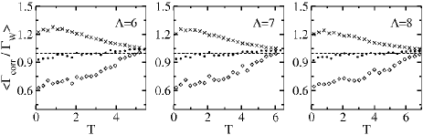
Figures 2 and 3 serve to quantify these statements. In a plot similar to that of Fig. 1, Fig. 2 shows the average of the ratios over the realizations versus for case I (center curve, circles), together with those for case II (upper curve, crosses) and case III (lower curve, diamonds). For all values of and the deviations of the average ratios from unity are largest for case III and smallest for case I. In the latter case the average ratio takes values above unity for small and tends to values close to but below unity even for large . In contrast, for case II the average ratio is larger, for case III it is smaller than unity for all values of . In all three cases, the deviations are largest for values between and . However, deviations from unity by more than percent occur only for or so. The curves rapidly tend to unity when approaches . Then all transmission coefficients take values close to unity.
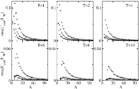
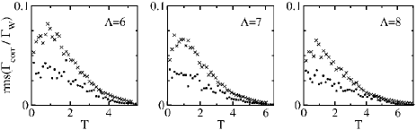
Figure 3 shows similarly the root mean square (rms) deviation of the ratio from unity (more precisely: the square root of the mean square deviation of the ratios from unity). That quantity takes the largest values for case III, and is very small unless . When approaches the rms values decrease rapidly for all three cases.
Because of the constraint only few points are at our disposal in the regime of largest deviations. For a more thorough test of the Weisskopf estimate we, therefore, also considered the case where is fixed and is varied. In Fig. 4 we show the averages of the ratios , with all transmission coefficients chosen equal, while in Figs. 5 and 6 cases I - III were considered as done above in Fig. 2. Again the deviations of from unity are largest for case III and smallest for case I. The average ratios are smaller than unity for all values of for case III (lower curve, diamonds) while for case I they are slightly smaller than unity for small and eventually reach a value slightly above unity when approaches , as is also observed in Fig. 2 for comparable values of and . For case II (upper curve, crosses) the deviations from unity are less than percent unless ; the ratio is above unity for all . The dependence of the curves on is similar to that for equally chosen transmission coefficients in Fig. 4 although for given values of and the latter deviate from unity much less than the former. As in Fig. 2 all curves in Fig. 5 tend to unity for close to .
In Fig. 6 we show the rms values for cases I and II. These are less than for all values of and that were considered. As suggested by Fig. 5 the rms values for case III are always larger than those for cases I and II but remain smaller than for . We do not show case III in order not to blur Fig. 5.
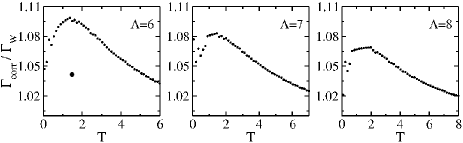
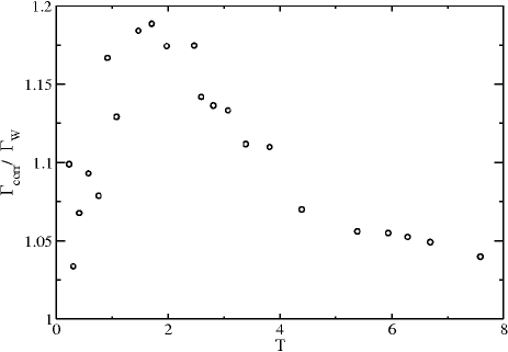
We also compared the Weisskopf estimate with data from a microwave experiment described in Refs. [5, 20]. The transmission amplitudes and the reflection amplitudes of microwaves coupled into and out of a flat resonator via two antennas were measured. The resonator had the shape of a tilted stadium billiard whose classical dynamics is chaotic [21]. The transmission coefficients associated with the two antennas were determined via the relation from the reflection spectra. Here the angular bracket denotes a frequency average. To this end the spectra, which exhibit isolated resonances for low frequencies and increasingly overlapping resonances with increasing frequency, were devided into frequency intervals of equal size. Dissipation into the walls of the resonator was accounted for by introducing weakly coupled fictitious channels with equal transmission coefficients where for . Hence channels and are the dominant ones in these experiments, as in case II. The transmission coeffcients of the absorptive channels were determined from a fit of the analytic expression for the autocorrelation function to the experimental one [7]. The width of the best fit yields while is computed from the resulting transmission coefficients and Eq. (1). From the measured spectra we thus obtained altogether values for the ratios . These are shown in Fig. 7. For they are very close to unity, as expected for a large number of weakly coupled channels. They approach a maximum for and then decrease again. For the deviations of the ratios from unity are around per cent. The ratios are larger than unity for all values of , in agreement with the numerical results for case II. Thus, in these experiments underestimates the correlation width. The deviations of the Weisskopf estimate from are similar for the sets of transmission coefficients resulting from other microwave experiments described in Ref. [22]. In another experiment [23] a superconducting chaotic microwave billiard was used, and dissipation by the walls was negligible. In that experiment three attennas were attached to the resonator so that . In Ref. [23] the transmission coefficients are determined from the partial widths of the measured resonances. Their sum yields while is determined from the experimental autocorrelation function shown in Fig. 4 of Ref. [23]. This yields , in good agreement with our numerical results for small values of and .
From the results obtained with the non-sorted transmission coefficients we conclude that the Weisskopf estimate Eq. (1) constitutes a good approximation to for practically all values of . Maximal deviations occur for small values of and unless . That statement applies also when incident and outgoing channel are the dominant ones (case II). The largest deviations are observed when these are the most weakly coupled channels (case III). In cases I and II relative deviations of from unity larger than percent are only observed for . Generally, for or for the deviations are less than percent and decrease rapidly with increasing or . We have shown that our results are relevant for the microwave experiments described in Refs. [5, 20, 22, 23]. It would be interesting to perform similar tests on the data obtained, for instance, in the experiments in Refs. [24, 25].
Acknowledgement
This work was supported through the SFB 634 by the DFG.
References
- [1] G. E. Mitchell, A. Richter, and H. A. Weidenmüller, Rev. Mod. Phys. 82 (2010) 2845, and arXiv 1001.2422
- [2] J. J. M. Verbaarschot, H. A. Weidenmüller, and M. R. Zirnbauer, Phys. Rep. 129 (1985) 367.
- [3] E. D. Davis and D. Boosé, Phys. Lett. B 211 (1988) 379.
- [4] E. D. Davis and D. Boosé, Z. Physik A 332 (1989) 427.
- [5] B. Dietz, H. L. Harney, A. Richter, F. Schäfer, and H. A. Weidenmüller, Phys. Lett. B 685 (2010) 263.
- [6] J. M. Blatt and V. F. Weisskopf, Theoretical Nuclear Physics, J. Wiley and Sons, New York 1952.
- [7] B. Dietz, T. Friedrich, H. L. Harney, M. Miski-Oglu, A. Richter, F. Schäfer, and H. A. Weidenmüller, Phys. Rev. E 81 (2010) 036205.
- [8] P. A. Moldauer, Phys. Rev. 177 (1969) 1841.
- [9] M. Simonius, Phys. Lett. B 52 (1974) 279.
- [10] Y. V. Fyodorov and B. A. Koruzhenko, Phys. Rev. Lett. 83 (1999) 65.
- [11] H. J. Sommers, Y. V. Fyodorov, and M. Titov, J. Phys. A 32 (1999) L77.
- [12] P. A. Moldauer, Phys. Rev. C 11 (1975) 426.
- [13] T. A. Brody, J. Flores, J. B. French, P. A. Mello, A. Pandey, and S. S. M. Wong, Rev. Mod. Phys. 53 (1981) 385.
- [14] G. L. Celardo, F. M. Izrailev, V. G. Zelevinsky, and G. P. Berman, Phys. Rev. E 76 (2007) 031119.
- [15] K. M. Frahm, H. Schomerus, M. Patra, and C. W. J. Beenakker, Europhys. Lett. 49 (2000) 48.
- [16] H. Schomerus, K. M. Frahm, M. Patra, and C. W. J. Beenakker, Physica A 278 (2000) 469.
- [17] T. Ericson, Phys. Rev. Lett. 5 (1960) 430 and Ann. Phys. (N.Y.) 23 (1963) 390.
- [18] J. J. M. Verbaarschot, Ann. Phys. 168 (1986) 368.
- [19] A. Müller and H. L. Harney, Z. Phys. A 337 (1990) 465.
- [20] B. Dietz, T. Friedrich, H. L. Harney, M. Miski-Oglu, A. Richter, F. Schäfer, and H. A. Weidenmüller, Phys. Rev. E 78 (2010) 055204(R).
- [21] H. Primack and U. Smilansky, J. Phys. A 27 (1994) 4439.
- [22] R. Schäfer, T. Gorin, T. H. Seligman, and H.-J. Stöckmann, J. Phys. A 36 (2003) 3289.
- [23] H. Alt, H.-D. Gräf, H. L. Harney, R. Hofferbert, H. Lengeler, A. Richter, P. Schardt, and H. A. Weidenmüller, Phys. Rev. Lett. 74 (1995) 62.
- [24] S. Hemmady, X. Zheng, T. M. Antonsen, Jr., E. Ott and S. M. Anlage, Phys. Rev. E 71 (2005) 056215.
- [25] O. Hul, O. Tymoshchuk, S. Bauch, P. M. Koch, and L. Sirko, J. Phys. A 38 (2005) 10489.