The HETDEX Pilot Survey. II. The Evolution of the Ly$\alpha$ Escape Fraction from the UV Slope and Luminosity Function of $1.9<$z$<3.8$ LAEs

Abstract

We study the escape of Ly$\alpha$ photons from Ly$\alpha$ emitting galaxies (LAEs) and the overall galaxy population using a sample of 99 LAEs at $1.9<z<3.8$ detected through integral-field spectroscopy of blank fields by the HETDEX Pilot Survey. For 89 LAEs with broad-band counterparts we measure UV luminosities and UV slopes, and estimate $E(B-V)$ under the assumption of a constant intrinsic UV slope for LAEs. These quantities are used to estimate dust-corrected star formation rates ($SFR$). Comparison between the observed Ly$\alpha$ luminosity and that predicted by the dust-corrected $SFR$ yields the Ly$\alpha$ escape fraction. We also measure the Ly$\alpha$ luminosity function and luminosity density ($\rho_{Ly\alpha}$) at $2<z<4$. Using this and other measurements from the literature at $0.3<z<7.7$ we trace the redshift evolution of $\rho_{Ly\alpha}$. We compare it to the expectations from the star-formation history of the universe and characterize the evolution of the Ly$\alpha$ escape fraction of galaxies. LAEs at $2<z<4$ selected down to a luminosity limit of $L(Ly\alpha)>3-6\times 10^{42}$ erg s^-1 (0.25 to 0.5 $L^{*}$), have a mean $\langle E(B-V)\rangle=0.13\pm 0.01$, implying an attenuation of $\sim 70$% in the UV. They show a median UV uncorrected $SFR=11$ M_⊙yr^-1, dust-corrected $SFR=34$ M_⊙yr^-1, and Ly$\alpha$ equivalent widths ($EW$s) which are consistent with normal stellar populations. We measure a median Ly$\alpha$ escape fraction of $29$%, with a large scatter and values ranging from a few percent to 100%. The Ly$\alpha$ escape fraction in LAEs correlates with $E(B-V)$ in a way that is expected if Ly$\alpha$ photons suffer from similar amounts of dust extinction as UV continuum photons. This result implies that a strong enhancement of the Ly$\alpha$ $EW$ with dust, due to a clumpy multi-phase ISM, is not a common process in LAEs at these redshifts. It also suggests that while in other galaxies Ly$\alpha$ can be preferentially quenched by dust due to its scattering nature, this is not the case in LAEs. We find no evolution in the average dust content and Ly$\alpha$ escape fraction of LAEs from $z\sim 4$ to 2. We see hints of a drop in the number density of LAEs from $z\sim 4$ to 2 in the redshift distribution and the Ly$\alpha$ luminosity function, although larger samples are required to confirm this. The mean Ly$\alpha$ escape fraction of the overall galaxy population decreases significantly from $z\sim 6$ to $z\sim 2$. Our results point towards a scenario in which star-forming galaxies build up significant amounts of dust in their ISM between $z\sim 6$ and 2, reducing their Ly$\alpha$ escape fraction, with LAE selection preferentially detecting galaxies which have the highest escape fractions given their dust content. The fact that a large escape of Ly$\alpha$ photons is reached by $z\sim 6$ implies that better constraints on this quantity at higher redshifts might detect re-ionization in a way that is uncoupled from the effects of dust.

1 Introduction

Ly$\alpha$ photons are produced in large amounts in star forming regions, therefore it was predicted nearly half a century ago that the Ly$\alpha$ emission line at 1216Å should be a signpost for star-forming galaxies at high redshift (Partridge & Peebles, 1967). Actual observations of Ly$\alpha$ emitting (LAE) galaxies at high redshift had to wait for the advent of 8-10m class telescopes (Hu et al., 1998). A little more than a decade has passed since their discovery, and thanks to a series of systematic surveys at optical and near-infrared wavelengths, large samples of LAEs, usually containing from tens to a few hundred objects, have been compiled over a wide range of redshifts from $z\sim 2$ to $z\sim 7$ (eg. Cowie & Hu, 1998; Rhoads et al., 2000; Kudritzki et al., 2000; Malhotra & Rhoads, 2002; Ouchi et al., 2003; Gawiser et al., 2006a; Ajiki et al., 2006; Gronwall et al., 2007; Ouchi et al., 2008; Nilsson et al., 2009a; Finkelstein et al., 2009; Guaita et al., 2010; Hayes et al., 2010a; Ono et al., 2010; Adams et al., 2011). Space based ultra-violet (UV) observations have also been used to study Ly$\alpha$ emitting galaxies at lower redshifts, all the way down to the local universe (Kunth et al., 1998, 2003; Hayes et al., 2005, 2007; Atek et al., 2008; Deharveng et al., 2008; Cowie et al., 2010).

The intrinsic production of both Ly$\alpha$ and UV continuum photons in a galaxy is directly proportional to the number of ionizing photons produced by young stars, which is proportional to the star formation rate ($SFR$) (Kennicutt, 1998; Schaerer, 2003). In practice, we do not expect the observed Ly$\alpha$ luminosity of galaxies to correlate well with their $SFR$ because the resonant nature of the n=1-0 transition in hydrogen makes the escape of Ly$\alpha$ photons a non-trivial radiative process.

In principle, the large number of scatterings suffered by a Ly$\alpha$ photon before escaping the neutral medium of a galaxy increase its probability, with respect to that of continuum photons outside the resonance wavelength, of being absorbed by a dust grain. Hence, we would expect even small amounts of dust in a galaxy’s inter-stellar medium (ISM) to severely decrease the equivalent width ($EW$) of the Ly$\alpha$ line (Hummer & Kunasz, 1980; Charlot & Fall, 1993). In reality the situation is far more complicated, and it is not clear how the extinction suffered by Ly$\alpha$, and that suffered by continuum photons, relate. One scenario which has been proposed by several authors (Neufeld, 1991; Haiman & Spaans, 1999; Hansen & Oh, 2006) is the possible enhancement of the Ly$\alpha$ $EW$ due to the presence of a very clumpy dust distribution in a multi-phase ISM. For this type of ISM geometry most of the dust lives in cold neutral clouds embedded in an ionized medium. In this scenario, Ly$\alpha$ photons have a high probability of being scattered in the surfaces of these clouds, spending most of their time prior to escape in the inter-cloud medium and actually suffering less dust extinction than non-resonant radiation, which can penetrate into the clouds where it has a higher chance of being absorbed or scattered by dust grains. Recently, Finkelstein et al. (2009) claimed that this process can simultaneously explain the Ly$\alpha$ fluxes and continuum spectral energy distributions of many objects in their sample of LAEs at $z\sim 4.5$.

At high redshift the Ly$\alpha$ line can also be affected by scattering in the inter-galactic medium (IGM), as escaping Ly$\alpha$ photons bluewards of the line center can be redshifted into the resonance wavelength. This effect is particularly important at $z>5$ as the density of neutral gas in the universe increases, but even at lower redshifts, when the universe is almost completely ionized, intervening Ly$\alpha$ forest absorption can occur. To first order, the IGM transmission blue-wards of Ly$\alpha$ is $\sim 90$%, 70%, and 50% at $z\sim 1.9$, 3.0, and 3.8 respectively (Madau, 1995). In the naive case where the line profile escaping a galaxy is symmetric and centered at the Ly$\alpha$ resonance, since only photons bluewards of the line are affected, we can expect attenuations of $\sim 5$%, 15%, and 25% on the emerging flux at these redshifts. In reality the process can be significantly different. While inflow of IGM gas onto galaxies can introduce further attenuation red-wards of the line resonance (Dijkstra et al., 2007), outflows in a galaxy’s ISM can redshift the emerging spectrum so as to be completely unaffected by the IGM (Verhamme et al., 2008). For example, in a sample of 11 LBGs and LAEs at $z\sim 3-5$, Verhamme et al. (2008) find no need to introduce IGM absorption to successfully fit the observed line profiles. This, combined with the inherent stochasticity of intervening absorption systems towards different lines of sight, makes Ly$\alpha$ IGM attenuation corrections very difficult and uncertain.

The kinematics of the neutral gas inside a galaxy and in its immediate surroundings also play an important role regarding the escape of Ly$\alpha$ photons (Verhamme et al., 2006; Dijkstra et al., 2006; Hansen & Oh, 2006; Dijkstra et al., 2007; Verhamme et al., 2008; Adams et al., 2009; Laursen et al., 2010; Zheng et al., 2010). Simply put, the velocity field of the neutral gas has a strong influence on the emission line profile of the Ly$\alpha$ line. Different combinations of geometry and velocity fields can “move” photons out of the resonance frequency either by blueshifting (typically due to in-falling gas) or redshifting (due to outflows) them, changing the number of scatterings photons experience before exiting the galaxy as well as their escape frequency. This process can affect the amount of dust extinction as well as the amount of potential IGM scattering those photons will suffer.

No clear agreement is found in the literature regarding the amount of dust present in the ISM of Ly$\alpha$ emitting galaxies. While most studies of narrow-band selected LAEs at $z\sim 3$ seem to indicate they are consistent with very low dust or dust-free stellar populations (Gawiser et al., 2006a, 2007; Nilsson et al., 2007; Gronwall et al., 2007; Ouchi et al., 2008), there have been recent results suggesting that the LAE population is more heterogeneous and includes more dusty and evolved galaxies, especially at lower redshifts (Lai et al., 2008; Nilsson et al., 2009a; Finkelstein et al., 2009).

We use a new sample of spectroscopically detected LAEs at $1.9<z<3.8$ from the The Hobby Eberly Telescope Dark Energy Experiment (HETDEX) Pilot Survey (Adams et al., 2011) to investigate the shape of the UV continuum of LAEs, as well as the Ly$\alpha$ luminosity function of these objects, and to address:

• The dust content of LAEs, parameterized by the dust reddening $E(B-V)$, and its evolution with redshift.

• The star-formation properties ($SFR$), the Ly$\alpha$ escape fraction in LAEs, and its evolution with redshift.

• The relation between the dust content and the escape fraction of Ly$\alpha$ photons.

• The relation between the dust extinction seen by continuum and resonant Ly$\alpha$ photons.

• The contribution of LAEs to the integrated star formation rate density at different redshifts.

• The Ly$\alpha$ escape fraction of the overall galaxy population and its evolution with redshift.

These galaxies have been detected through wide integral-field spectroscopic mapping of blank fields, using the Visible Integral-field Replicable Unit Spectrograph Prototype (VIRUS-P, Hill et al., 2008). The Pilot Survey catalog of emission line galaxies is presented in Adams et al. (2011), hereafter Paper I. The large redshift range spanned by our sample allows us to check for any potential evolution in the above properties of LAEs.

In §2 we describe the HETDEX Pilot Survey from which the sample of Ly$\alpha$ emitting galaxies is drawn. In §3 we present our sample of LAEs along with their luminosities and redshift distribution. §4 presents our measurement of the UV continuum slope and derivation of the amount of dust extinction present in these objects. Discussion of any potential evolution in the dust properties of LAEs is also in this section. We compare both uncorrected as well as dust-corrected $SFR$s derived from both UV and Ly$\alpha$ in §5, where we also compute the escape fraction of Ly$\alpha$ photons and show how it depends on the amount of dust reddening. In §6 we present the Ly$\alpha$ luminosity function and check for its possible evolution with redshift. We compare the integrated $SFR$ density derived from the Ly$\alpha$ luminosity function to that for the global galaxy population in §7. In this way we can assess the contribution of LAEs to the star-formation budget of the universe at these redshifts and estimate the Ly$\alpha$ photon escape fraction for the overall galaxy population. Finally, we summarize our results and present our conclusions in §8.

Throughout the paper we adopt a standard set of $\Lambda$CDM cosmological parameters, $H_{o}=70$ km s^-1Mpc^-1, $\Omega_{M}=0.3$, and $\Omega_{\Lambda}=0.7$ (Dunkley et al., 2009).

2 The HETDEX Pilot Survey

Ever since their discovery, the standard method for detecting and selecting LAEs has been through narrow-band imaging in a passband sampling the Ly$\alpha$ line at a given redshift. The redshift range of these type of surveys is given by the width of the narrow-band filter used, and is typically of the order of $\Delta z=0.1$. Hence, these studies are limited to very narrow and specific redshift ranges. In terms of surveyed volumes this limitation is compensated by the large fields of view of currently available optical imagers which allow for large areas of the sky ($\sim 1$deg²) to be surveyed using this technique.

An alternative technique, which has been attempted for detecting LAEs over the last few years, is to do so through blind spectroscopy. This can be done either by performing very low resolution slit-less spectroscopy (Kurk et al., 2004; Deharveng et al., 2008), blind slit spectroscopy (Martin & Sawicki, 2004; Tran et al., 2004; Rauch et al., 2008; Sawicki et al., 2008; Cassata et al., 2011), or integral-field spectroscopy (van Breukelen et al., 2005).

The success of this type of surveys has been variable. While early attempts to detect LAEs at $z\sim 6$ using slit spectroscopy failed to do so, and could only set upper limits to their number density (Martin & Sawicki, 2004; Tran et al., 2004), more recent attempts at lower redshifts ($2<z<6$) like the ones by Rauch et al. (2008) and Cassata et al. (2011), have produced large samples of objects. Similarly, an early attempt by Kurk et al. (2004) to find LAEs at $z=6.5$ using slit-less spectroscopy only yielded one detection, while more recently space-based UV slit-less spectroscopy with the GALEX telescope has allowed for the construction of a large sample of LAEs at $z\sim 0.3$ (Deharveng et al., 2008). The only attempt to detect LAEs using integral-field spectroscopy previous to this work was done by van Breukelen et al. (2005), who used the Visible Multi-Object Spectrograph (VIMOS) integral field unit (IFU) on the Very Large Telescope (VLT) to build a sample of 18 LAEs at $2.3<z<4.6$ over an area of 1.44 arcmin² corresponding to the VIMOS IFU field-of-view.

Although when doing spectroscopic searches for LAEs the wavelength range, and hence the redshift over which Ly$\alpha$ can be detected, is tens of times larger than for narrow-band imaging, surveyed volumes have been typically small due to the small areas sampled by the slits on the sky, or the small fields-of-view of most integral field units. For example, the IFU survey by van Breukelen et al. (2005) only covered $\sim 10^{4}$Mpc³ because of the small area surveyed, while the $z\simeq 3.1$ narrow-band survey by Gronwall et al. (2007) covered $\sim 10^{5}$Mpc³ over a very narrow range of $\Delta z=0.04$ because of the large $36^{\prime}\times 36^{\prime}$ area which can be imaged with the MOSAIC-II camera. It is clear that the most efficient way of building large samples of LAEs would be to conduct spectroscopic searches over large areas of the sky.

HETDEX (Hill et al., 2008) will survey $\sim 60$ deg² of sky using the Visible Integral-field Replicable Unit Spectrograph (VIRUS, Hill et al., 2010), a wide field of view ($16^{\prime}\times 16^{\prime}$) integral field spectrograph currently being built for the 9.2m Hobby Eberly Telescope (HET). HETDEX will produce a sample of $\sim 8\times 10^{5}$ LAEs at $1.9<z<3.5$ over a volume of 8.7 Gpc³. The power-spectrum of the spatial distribution of these objects will be used to set a percent level constrain on the dark energy equation of state parameter $w$ at these high redshifts (Hill et al., 2008). A prototype of the instrument, VIRUS-P, is currently the largest field-of-view IFU in existence, and has been used over the last 3 years to conduct a Pilot Survey for LAEs from which the sample used in this work is taken from (Paper I). The Pilot Survey, described below, samples the $1.9<z<3.8$ range, and covers a volume of $\sim 10^{6}$ Mpc³ over an area of 169 arcmin². This volume is ten times larger than the one covered in Gronwall et al. (2007) and Guaita et al. (2010), three times larger than the one covered by Nilsson et al. (2009a), and of comparable size to the one sampled at $z=3.1$ by Ouchi et al. (2008) but over an area 20 times smaller, exemplifying the power of integral field spectroscopy to search for emission line galaxies over large volumes.

The HETDEX Pilot Survey obtained integral field spectroscopy over $\sim$169.23 arcmin² of blank sky in four extra-galactic fields (COSMOS: 71.6 arcmin², GOODS-N: 35.5 arcmin², MUNICS-S2: 49.9 arcmin², and XMM-LSS: 12.3 arcmin²; Scoville et al., 2007; Dickinson et al., 2003; Drory et al., 2001; Pierre et al., 2004) using VIRUS-P on the 2.7m Harlan J. Smith telescope at McDonald Observatory. The goal of the survey is to conduct an unbiased search for spectroscopically-detected emission line galaxies over a wide range of redshifts. Although a powerful dataset itself, the Pilot Survey also provides a proof of concept and a crucial test-bench for the planned HETDEX survey.

The observations and data reduction, as well as the detection and classification of emission line galaxies, are presented in Paper I, and we refer the reader to it for a more detailed description of the survey design. Briefly, each field is mapped by a mosaic of $1.7^{\prime}\times 1.7^{\prime}$ VIRUS-P pointings (27, 13, 16, and 4 pointings in COSMOS, GOODS-N, MUNICS-S2, and XMM-LSS respectively). The VIRUS-P IFU consists of an square array of 246 fibers, each 4.235^′′ in diameter, sampling the field with a 1/3 filling factor. While a set of three dithered exposures covers the field-of-view almost completely, we observed each pointing at six dithered positions, ensuring complete coverage and improving the spatial sampling of the field and the astrometric accuracy of our detections. For each pointing, we obtained spectra at 1,476 ($6\times 246$) positions, with any point on the sky being typically sampled by 2 overlapping fibers. Overall, the Pilot Survey consists of $\sim$88,000 individual spectra over 169 arcmin² of blank sky. Each spectrum covers the 3600Å-5800Å wavelength range with $\sim 5$Å FWHM resolution ($\sigma_{inst}\sim 130$ km s^-1 at 5000Å).

After the data are reduced and a 1D flux-calibrated spectrum is extracted for each fiber position, we search the “blank” spectra for emission lines using an automated procedure (Paper I). Line detections are associated, when possible, with counterparts in broad-band images available for all four fields. The VIRUS-P wavelength range allows the detection of common strong emission lines present in star-forming galaxies such as Ly$\alpha$ at $1.9<z<3.8$, [OII]$\lambda$3727 at $z<0.56$, H$\beta$ at $z<0.19$, [OIII]$\lambda$4959 at $z<0.17$, [OIII]$\lambda$5007 at $z<0.16$, as well as typical AGN lines like CIV$\lambda$1549 at $1.3<z<2.7$, CIII]$\lambda$1909 at $0.9<z<2.0$, and MgII$\lambda$2798 at $0.3<z<1.1$.

Source classification is based on the presence of multiple spectral lines when available. In the case of single line detections, the spectral classification is considerably more challenging. For LAEs, only the Ly$\alpha$ line appears in our wavelength range, so we expect single line detections for our objects of interest. Nevertheless, [OII] emitters at $0.19<z<0.56$ will also appear as single line detections in the VIRUS-P spectra. Even [OII] emitters at $z<0.19$ that have unfavorable emission line ratios can appear as single line detections if H$\beta$ and the [OIII] doublet are below the noise level. Our 5Å FWHM spectral resolution is not high enough to resolve the [OII]$\lambda$3727 doublet, so we cannot rely on the line profile to classify these objects. While galaxies detected in redder lines such as H$\beta$ and [OIII]$\lambda$5007 can also appear as single line detections depending on their redshifts and line ratios, the volume over which we sample these galaxies is $\sim 400$ times smaller than the volume over which we sample LAEs, and $\sim 20$ times smaller than the volume over which we sample [OII] emitters. Hence, contamination from H$\beta$ and [OIII] emitters is negligible.

The classification of single line detections is thoroughly discussed in Paper I, and is based on an $EW$ criterion, where objects showing rest-frame $EW(Ly\alpha)>20$Å are classified as LAEs (for 4 objects the $EW>20$Å criterion was bypassed due to the existence of further evidence pointing towards their LAE nature; see Paper I). This $EW$ constraint effectively reduces the contamination from low-z interlopers to a negligible level. A total of 105 Ly$\alpha$ detections are present in the Pilot Survey catalog presented in Paper I. Of these, 6 show X-ray counterparts indicating an AGN nature, leaving a final sample of 99 “normal” star-forming LAEs. In Paper I we also present a thorough assessment of the completeness and spurious source contamination in our catalog, based on simulated data. The completeness is used in §6 to estimate the Ly$\alpha$ luminosity function. In our sample of LAEs we expect a 4-10% contamination from spurious sources. The sample used in this work is presented in Table 1.

3 LAE Sample

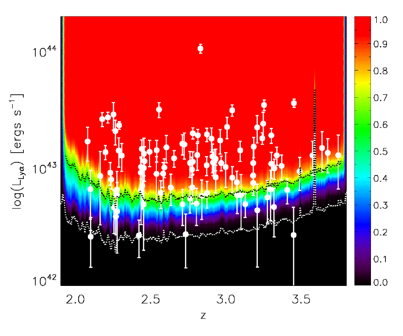
Figure 1: Limiting Ly$\alpha$ luminosity ($5\sigma$) as a function of redshift for the survey. The survey depth varies across the observed area due to changes in atmospheric transparency, Galactic extinction, and instrumental configuration. Hence, the background color indicates the fraction of the total survey area over which a given limit is reached. White points mark the redshift and Ly$\alpha$ luminosities (with error-bars) of the 99 objects classified as LAEs. The dotted black and white lines show the mean and best limits over the whole survey respectively. Even below this last limit, the completeness of the survey is not zero, explaining why we see 2 points below this curve.

The 99 LAEs in the sample span a range in luminosities of ${\rm log}(L_{Ly\alpha})=42.42-44.03$, and have a median luminosity of ${\rm log}(\tilde{L}_{Ly\alpha})=43.03$. Figure 1 shows the survey 5$\sigma$ limiting Ly$\alpha$ luminosity as a function of redshift, together with the luminosities and redshifts of all LAEs in the sample. The depth of the observations is variable across the survey area and dependent on the observing conditions, the airmass at which the observations were taken, the Galactic dust extinction towards different fields, and the instrumental configuration. Colors in Figure 1 correspond to the fraction of the total surveyed area for which the spectra reaches the corresponding limit in luminosity. While VIRUS-P has its lower throughput in the blue end of the wavelength range, the smaller luminosity distance at lower redshifts compensates for this fact, providing a relatively flat luminosity limit throughout the entire redshift range. As mentioned above, detailed simulations quantifying the completeness and spurious detection ratio for the whole survey are presented in Paper I. A good understanding of the completeness of the survey is essential in order to calculate the Ly$\alpha$ luminosity function. As shown in Paper I, the completeness at the 5$\sigma$ flux limit shown in Figure 1 is 33%, reaching 50% at 5.5$\sigma$ and 90% at 7.5$\sigma$.

The redshift distribution of LAEs in our sample is shown in Figure 2 (errorbars show Poisson statistical uncertainties). The detected galaxies span a range in redshift of $2.079<z<3.745$, with a median redshift of $\tilde{z}=2.811$, properly sampling the $1.9<z<3.8$ range over which they could be detected. Figure 2 also shows the predicted redshift distribution of LAEs in the Pilot Survey calculated by integrating the Gronwall et al. (2007) luminosity function of narrow-band selected LAEs at $z=3.1$ above the Pilot Survey flux limits shown in Figure 1, and correcting for the survey completeness. The agreement is excellent at high redhsift ($z>3$), but we observe a drop in the number of LAEs at lower redhsifts from what is predicted by a non-evolving luminosity function. Recent narrow-band studies of $z\sim 2$ LAEs show hints for both an increase (Guaita et al., 2010) and decrease (Nilsson et al., 2009a) of the LAE number density from $z=3$ to $z=2$. As stated by the authors themselves, neither of these studies probe a large enough volume to allow for a significant detection of the evolution in the LAE number density. In our surveyed volume, which is a few times larger than the volumes surveyed in those studies, we find some evidence for a decrease in the number density of LAEs from $z\sim 4$ to $z\sim 2$, although as discussed in §6, the statistical uncertainties remain too large to make a definitive statement. In any case, this type of evolution is expected if the escape fraction of Ly$\alpha$ photons from galaxies decreases towards lower redshifts. In §7 we find evidence that this effect indeed occurs, which supports the observed drop in the LAE number density.

4 The UV slope of Lyman alpha emitters

The UV continuum slope has been shown to be a powerful tool for estimating the amount of dust extinction in star-forming galaxies in the local universe (Meurer et al., 1995, 1999) as well as at high redshift (Daddi et al., 2004; Bouwens et al., 2009; Reddy et al., 2010). Direct observations of the ultra-violet spectral energy distribution of local star-forming galaxies have demonstrated that in the 1000Å-3000Å range, they are very well described by a power-law spectrum of the form $f_{\lambda}\propto\lambda^{\beta}$ (Calzetti et al., 1994). Differential dust extinction (reddening) makes the power-law slope correlate well with the amount of dust extinction in galaxies.

Measuring the spectral slope of the UV SED of LAEs at $1.9<z<3.8$ provides a direct measurement of their dust content, and its evolution with time. Knowledge of the amount of dust extinction in LAEs allows us to correct UV measured $SFRs$. An unbiased measurement of the $SFR$ in these objects is not only important regarding the star-formation properties of these galaxies, but can also be used, together with the observed Ly$\alpha$ luminosities, to estimate the escape fraction of Ly$\alpha$ photons from the ISM of these high redshift systems, and to study a possible evolution in this quantity.

4.1 Measurement of the UV continuum Slopes, UV Luminosities, and Ly$\alpha$ EWs

We identify continuum counterparts of spectroscopically detected LAEs in our sample using publicly available broad-band optical images sampling the rest-frame UV SED of the objects. Multi-band aperture photometry is then used to measure their UV continuum slope ($\beta$) and UV luminosity as described below.

For the purpose of measuring $\beta$ we use the B, r⁺, i⁺, and z⁺ images of the COSMOS and GOODS-N fields presented in Capak et al. (2004) and Capak et al. (2007), the g, r, i, and z images of the XMM-LSS field from the Canada-France-Hawaii Telescope Legacy Survey (CFHTLS, Mellier et al., 2008) W1 field, and the g, i, and z MUNICS-Deep images presented in Paper I. The identification and association with broad-band counterparts of our emission line detected objects makes use of a maximum likelihood algorithm which is described in detail in Paper I. Briefly, our astrometric uncertainty and the typical surface density of galaxies as a function of continuum brightness is used to identify the most likely broad-band counterpart for each LAE. The possibility of the emission-line source having no counterpart in the broad-band imaging is also considered. This can happen if the source is fainter than the sensitivity of the images or if the source is spurious. The no counterpart option is adopted if the probability exceeds that of all other possible counterparts. Only 9 out of 99 (9%) objects show no broad-band counterparts. This number is in good agreement with the 4-10% contamination expected from spurious detections in our LAE sample (Paper I, §3), although these objects could in principle be real and have very high $EW$s. In Paper I we showed that only one of them has significantly high $EW$ given the limits that can be put using the depth of the broad-band images, while the large majority (8/9) show low signal-to-noise (S/N) detections ($<6.5$) where the false detection ratio is the highest. For simplicity we omit these “no counterpart” sources from our analysis as we expect the large majority of them to be false detections. We also reject one other object (HPS-89) from our analysis because its broad-band counterpart photometry is catastrophically affected by a bright neighbor.

Fluxes are measured in optimal $1.4\times$FWHM diameter color apertures, and scaled to total fluxes for each object using the ratio between V-band (g-band for MUNICS) fluxes measured in the color aperture and aperture-corrected fluxes measured in a SExtractor (Bertin & Arnouts, 1996) defined Kron aperture (Gawiser et al., 2006a; Blanc et al., 2008). Any contribution from the measured Ly-alpha line to the broad-band fluxes is removed. While we do take into account IGM absorption when fitting for the UV slope, we decide to omit the U-band in the fits because in our redshift range the band includes the Lyman 912Å break. Since IGM absorption is expected to be stochastic, an average line-of-sight correction might not apply to single objects. This leaves us with a B-band through z-band SED for each object.

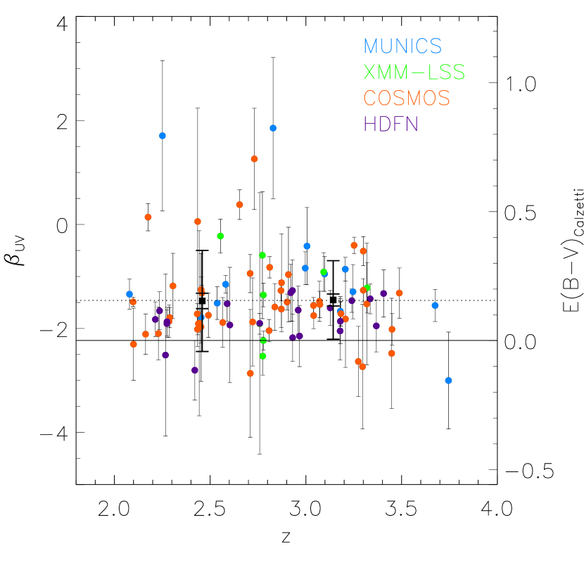
Figure 3: UV continuum slope as a function of redshift for the 89 LAEs with broad-band optical counterparts. Objects are color coded by field. The right axis shows the equivalent E(B-V) assuming a Calzetti et al. (2000) attenuation law. The horizontal lines mark the assumed intrinsic UV slope corresponding to a dust-free stellar population ($\beta_{0}=-2.23$, solid line), and the mean for the whole sample (dotted line). Also shown are the mean UV slopes for two redshift bins at $1.9<z<2.8$ and $2.8<z<3.8$ (black squares), with two sets of error-bars corresponding to the standard deviation in $\beta$ within each bin (large error-bars) and the formal error in the mean (small error-bars).

The approximate rest-frame wavelength range sampled by the above bands shifts from 1500Å-3000Å at $z=1.9$ to 900Å-1900Å at $z=3.8$, so only the B-band is affected by Lyman forest absorption at the higher redshift end of our range. Following a similar methodology as that described in Meurer et al. (1999) and Reddy et al. (2010), we compute the UV continuum slope for each object by fitting the rest-frame UV SED with a power-law spectrum of the form $f_{\lambda}\propto\lambda^{\beta}$ corrected for IGM absorption at the corresponding redshift of each object using a Madau (1995) prescription. All available bands redwards the Lyman break are used to perform the fit. When an object is not detected in a particular band, we properly include the upper limit in flux given by the photometric uncertainty in the $\chi^{2}$ minimization in order to not censor our data. The error in $\beta$ is estimated from Monte Carlo simulations of 100 realizations of the UV SED, where the fluxes in each band are varied within their photometric errors. This fitting also provides the UV luminosities at 1216Å and 1500Å which are used to estimate the Ly$\alpha$ $EW$ and the $SFR$, respectively. All these quantities are reported in Table 1. Figure 3 shows the UV continuum slope $\beta$ as a function of redshift for the 89 objects having continuum counterparts.

In principle, the UV slope can depend not only on the amount of dust extinction, but also on the age, metallicity, and initial mass function (IMF) giving rise to the stellar population. Extensive work can be found in the literature regarding these effects on the observed UV slope of star-forming galaxies. Leitherer & Heckman (1995) showed that for both instantaneous bursts and constant star formation synthetic stellar populations, changes of the order of $\Delta\beta=\pm 0.2$ around a typical value of $\beta\sim-2.3$ are introduced by variations in age (1 Myr to 1 Gyr) and metallicity ($0.1\;Z_{\odot}$ to $2\;Z_{\odot}$). They also find the UV slope to be largely insensitive to the assumed IMF. This result is in good agreement with the work of Bouwens et al. (2009), who demonstrate that the UV slope dependence on dust is dominant over that on age, metallicty and IMF. They use Bruzual & Charlot (2003) models to show that changes by a factor of two in age and metallicity introduce changes of $\Delta\beta\lesssim 0.1$. Schaerer & Pelló (2005) also present a similar result. In Figure 1 of their paper it can be seen that for a range in ages of 1 Myr to 1 Gyr (encompassing the expected age range for LAEs), and metallicities between 1/50 Z_⊙ and solar, both constant SFR population synthesis models, and single bursts younger than 10 Myr (time over which they can produce significant Ly$\alpha$ emission) show variations in their UV slopes of $\Delta\beta=\pm 0.2$ ($\Delta E(B-V)=0.04$). These systematics are smaller than the typical uncertainty in the measurement of $\beta$ for LAEs in our sample. Therefore, by assuming a constant value for the intrinsic (dust-free) UV slope across our LAE sample, we can robustly estimate the amount of dust reddening directly from the observed values of $\beta$ given an attenuation law.

The right axis of Figure 3 shows the corresponding value of the reddening $E(B-V)$, calculated assuming an intrinsic UV slope $\beta_{0}=-2.23$ for a dust-free stellar population (Meurer et al., 1999), and a Calzetti et al. (2000) extinction law. The value of $\beta_{0}$ is derived from a fit to the relation between the IR to UV ratio and $\beta$ in a sample of local starburst galaxies (Meurer et al., 1999), and reproduces the observed relation at $z\sim 2$ (Reddy et al., 2010). Although Reddy et al. (2010) found young ($<100$ Myr) $z\sim 2$ galaxies to lie slightly below the Meurer et al. (1999) relation, and closer to that of Pettini et al. (1998), these two relations converge at low extinction and imply basically indistinguishable values for $\beta_{0}$. In order to take into account age and metallicity induced uncertainties in our error budget for the dust reddening, we sum in quadrature a systematic error of $\Delta\beta=\pm 0.2$ ($\Delta E(B-V)=0.04$) to the uncertainty in $\beta$, and propagate it into the error in $E(B-V)$. Measured values for the dust reddening and it associated uncertainty are reported in Table 1.

4.2 Dust Properties of LAEs and comparison to Previous Measurements

Our LAEs show a mean UV continuum slope $\langle\beta\rangle=-1.5\pm 0.1$ (formal error on the mean) corresponding to a mean $\langle E(B-V)\rangle=0.16\pm 0.02$ (median $\tilde{E}(B-V)=0.13$). The measured slopes span a relatively broad range of $-3<\beta<+2$, with the large majority (83/89, 93%) of the objects having $\beta<0$ ($E(B-V)<0.45$). All objects with $\beta<\beta_{0}$ (i.e. bluer than the assumed intrinsic dust-free slope) are consistent with $\beta=\beta_{0}$ (i.e. $E(B-V)=0$) within 1$\sigma$.

These slopes and reddenings are in rough agreement with previous measurements of narrow-band detected LAE broad-band colors. For $z=2.1$ LAEs, Guaita et al. (2010) find a typical $(B-R)\simeq 0.2$ ($\beta=-1.5$ using equation 3 in Nilsson et al. (2009a)) and a relatively uniform distribution in the $-0.5<(B-R)<1$ ($-3.3<\beta<0.7$) range. Similarly, at $z=2.3$, Nilsson et al. (2009a) find a median $(B-V)=0.14$ corresponding to $\beta=-1.4$, with the bulk of their LAEs having $-3.0<\beta<2.0$. At $z=2.2$ Hayes et al. (2010a) used SED fitting to find that LAEs in their sample have a range in $E(B-V)=0-0.4$. At higher redshifts, usually lower levels of extinction are measured. At $z=3.1$ Nilsson et al. (2007) find $A_{V}=0.26^{+0.11}_{-0.17}$ from fitting the stacked SED of 23 LAEs in the GOODS-S field, corresponding to $E(B-V)=0.06^{+0.03}_{-0.04}$ (assuming a Calzetti attenuation law). Verhamme et al. (2008), using Monte Carlo Ly$\alpha$ radiative transfer fitting of the line profiles of 11 $z\sim 3-5$ LBGs (8 of them also LAEs) from Tapken et al. (2007), find that the color excess spans a range of $E(B-V)=0.05-0.2$. Gawiser et al. (2006a) report that the best-fit SED to the stacked optical photometry of $z=3.1$ LAEs in their sample has $A_{V}=0^{+0.1}_{-0.0}$, corresponding to $E(B-V)<0.03$.

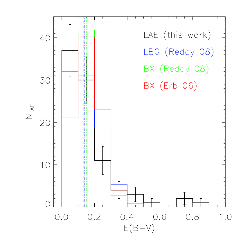
Figure 4: $E(B-V)$ distribution of LAEs in our sample (Poisson error-bars), together with that of BX/LBGs taken from Erb et al. (2006) and Reddy et al. (2008) (solid histograms). The median of each distribution is marked by the vertical dashed lines.

For comparison, similar ranges in $\beta$ and $E(B-V)$ as those seen here have been measured for LBGs (e.g. Shapley et al., 2001; Erb et al., 2006; Reddy et al., 2008). Figure 4 shows the $E(B-V)$ distribution of LAEs in our sample, compared with that of UV continuum selected galaxies at $1.9<z<2.7$ (BX galaxies) and at $2.7<z<3.4$ (LBGs) from Erb et al. (2006) and Reddy et al. (2008). The $E(B-V)$ distributions for the continuum-selected galaxies are different from those presented in the original papers in that we have set all their $E(B-V)<0$ values to zero for proper comparison with our sample. It can be seen that both the shape and median value of the $E(B-V)$ distribution of LAEs and BX/LBGs are relatively similar (medians are indicated by the dashed lines in Figure 4). This result, together with the fact that LAEs and BX/LBGs seem to overlap in the two-color BX/LBG selection diagram (Guaita et al., 2010; Gawiser et al., 2006a), implies that both populations have relatively similar spectral continuum properties in the UV. Nevertheless, Figure 4 shows an LAE distribution that is peaked at lower $E(B-V)$ than the BX/LBG distributions, and also that Ly$\alpha$ selection might allow for the inclusion of some highly reddened objects, although the reality of these red LAEs will be questioned in the next section. These galaxies, if real, are excluded of UV-selected samples by construction, since the color cuts in those selections reject object with $E(B-V)\gtrsim 0.5$ (Daddi et al., 2004; Blanc et al., 2008).

The observed UV slopes imply that LAEs present low levels of dust extinction. One third (30/89) of the LAEs in our sample are consistent with being dust-free ($E(B-V)=0$) to 1$\sigma$, with the fraction going up to 60% within the 2$\sigma$ uncertainty. Still, a significant fraction of LAEs show non negligible amounts of dust. As will be shown in §5, dust in LAEs should not be neglected; doing so would strongly underestimate the $SFR$ in these objects. Dust also plays a dominant role in setting the escape fraction of Ly$\alpha$ photons, as we will discuss in §5.4.

4.3 Evolution of the Dust Properties of LAEs

At first sight, Figure 3 shows different behaviors in the dust-content distribution of LAEs at the high and low redshift ends of our sample. At $z<3$ we see the emergence of a small population of LAEs (6/89) with red UV slopes ($\beta>0$). This objects, if real, could represent an interesting population of dusty star forming galaxies in which some physical mechanisms allows for the escape of Ly$\alpha$ photons. We have reasons to question the reality of these objects (see below). Furthermore, in this section we show that their presence does not affect the average properties of the LAE population which is dominated by UV-blue LAEs.

To test for any evolution on the dust-content of LAEs with redshift we divided the sample in two redshift bins: low-$z$ ($1.9<z\leq 2.8$) and high-$z$ ($2.8<z<3.8$). The division corresponds to the median redshift of the whole sample, and divides the survey volume in two roughly equal sub-volumes. The corresponding age of the universe at $z=3.8$, 2.8, and 1.9 is $\sim$1.6, 2.3, and 3.4 Gyr. The median Ly$\alpha$ luminosity of the two sub-samples equals that of the whole sample (log$L_{Ly\alpha}=$43.0).

The mean UV slopes of the high and low redshift samples are shown in Figure 3. Error-bars show the formal error on the mean and the standard deviation for each sample including $\sim$68% of the objects. The mean value of $E(B-V)$ stays constant with values $0.16\pm 0.03$ and $0.17\pm 0.02$ for the low and high redshift bins respectively. The scatter around these values is large and the means are statistically consistent with each other, and with the mean of the full sample. Therefore, we do not detect any significant evolution in the average UV slope and dust reddening of LAEs from $z\sim 4$ to $z\sim 2$.

The lack of evolution in the mean dust-content of LAEs implies that this rare population of very high $E(B-V)$ objects emerging at $z<3$, if real, does not affect the average properties of the overall population due to their reduced number. The dust content of the bulk of the LAE population remains relatively constant across the $2<z<4$ range.

Doubt regarding the validity of the UV slope measurements for these objects, and their classification as LAEs arises from looking at the distribution of rest-frame Ly$\alpha$ $EWs$ for our sample. Figure 5 shows the $EW$ distribution for both UV-blue ($\beta<0$) and UV-red ($\beta\geq 0$) LAEs together with the one for the whole sample. The Ly$\alpha$ $EW$ is measured as described in §4.1, and hence can differ from the values presented in Paper I. It is evident from Figure 5 that UV-blue LAEs dominate the overall population since they present a practically indistinguishable $EW$ distribution (well fitted by an exponential with an e-folding parameter $w_{0}=74\pm 7$) from that of the full sample ($w_{0}=77\pm 7$). UV-red LAEs on the other hand, in addition to being rare in numbers, present a very different distribution in rest-frame $EW$, characterized by the presence of many extremely high $EW$ ($>500$Å) objects. Two of these UV-red objects are in the MUNICS field where we lack deep X-ray data to reject AGNs from our sample (one of these sources shows significantly extended Ly$\alpha$ emission and is a good candidate for an extended Ly$\alpha$ nebula, or Ly$\alpha$ Blob as discussed in Paper I). The remaining four objects have low association probabilities ($\leq 0.6$) with their broad-band counterparts, casting doubt on the validity of our UV slope and $EW$ measurements for these objects. Further follow-up observations are necessary to confirm the nature of these detections.

If real, these UV-red LAEs would have an extreme nature, being very dusty and highly star-forming. We remove these six objects from all the subsequent analysis, and for the rest of the paper we focus only on the results regarding the dominant UV-blue LAE population. It must be kept in mind that if these objects happen to be real LAEs, no strong evidence for a bimodality in the dust content or $SFR$ of LAEs is found in our data. The $\beta>0$ cut used to separate this population of objects is solely based on the fact that $\beta>0$ objects are absent at $z>3$ in our sample. After removing these objects from our sample, we find a mean dust-reddening for LAEs of $\langle E(B-V)\rangle=0.13\pm 0.01$, corresponding to an average dust attenuation of $\sim 70$% at 1500Å.

5 UV versus Ly$\alpha$ $SFR$s and the Escape Fraction of Ly$\alpha$ Photons

In this section we use the dust extinction values derived from the UV continuum slope in the previous section to estimate the dust-corrected $SFR$ of LAEs in our sample. A comparison between the observed Ly$\alpha$ luminosity and the intrinsic Ly$\alpha$ luminosity implied by the dust-corrected $SFR$ allows estimation of the escape fraction of Ly$\alpha$ photons from these galaxies. Throughout this analysis we have decided to neglect the effects of the IGM. As stated in §1, at these redshifts we expect attenuations for Ly$\alpha$ of no more than 5-25%, which is within our typical uncertainty for the Ly$\alpha$ luminosity. Furthermore, if outflows are common in LAEs, as many lines of evidence suggest, then IGM scattering at these redshifts may become even less important as most Ly$\alpha$ photons leave galaxies red-shifted from the resonance wavelength (see discussion and references in §1). We start by comparing the observed (not corrected for dust) $SFRs$ derived from the UV and Ly$\alpha$ luminosities, then introduce the dust corrections, and finally estimate the escape fraction of Ly$\alpha$ photons and study how it relates to the amount of dust reddening.

5.1 Estimation of the Star Formation Rate and the observed $SFR(Ly\alpha)$ to $SFR(UV)$ ratio.

The UV monochromatic luminosity at 1500Å ($L_{\nu,1500}$) for each object is taken from the fits described in §4. In order to calculate the $SFR$ we use a standard Kennicutt (1998) conversion

$$SFR(UV)\;[{\rm M_{\odot}yr^{-1}}]=1.4\times 10^{-28}L_{\nu,1500}[\rm{erg\;s^{-1}Hz^{-1}}]$$ (1)

which assumes a Salpeter IMF with mass limits 0.1 to 100 M_⊙. The Ly$\alpha$ derived $SFRs$ were calculated using the standard Kennicutt (1998) conversion factor for H$\alpha$ and assuming the intrinsic Ly$\alpha$ to H$\alpha$ ratio of 8.7 from Case B recombination theory (Brocklehurst, 1971; Osterbrock & Ferland, 2006), so

$$SFR(Ly\alpha)\;[{\rm M_{\odot}yr^{-1}}]=7.9\times 10^{-42}\frac{L_{Ly\alpha}}{8.7}[\rm{erg\;s^{-1}}]$$ (2)

Figure 6 shows $SFR(Ly\alpha)$ versus $SFR(UV)$ for our 83 objects. Without accounting for dust we measure median $SFRs$ of 11 M_⊙yr^-1 and 10 M_⊙yr^-1 from UV continuum and Ly$\alpha$ respectively. Although these agree with what is typically quoted for LAEs in the literature, we consider them to be underestimated by roughly a factor of $\sim 3-4$ because of the lack of a dust extinction correction.

We observe a median ratio $SFR(Ly\alpha)/SFR(UV)=0.83$. Single objects present a large scatter around the median, with values ranging from 0.2 to 5.9. Since the UV $SFR$ conversion factor is valid for galaxies with constant star formation over $100$ Myr or more, while the one for Ly$\alpha$ is valid at much younger ages of $\sim 10$ Myr (Kennicutt, 1998), young galaxies can have intrinsic $SFR(Ly\alpha)$ to $SFR(UV)$ ratios higher than unity. The dashed lines in Figure 6 show the allowed range for dust-free constant star-formation stellar populations with metallicities from 1/50 Z_⊙ to solar and ages from 1 Myr to 1 Gyr from Schaerer (2003). A Ly$\alpha$ escape fraction of less than unity can push objects above this range. All the objects in our sample show $SFR(Ly\alpha)$ to $SFR(UV)$ ratios (or roughly equivalently Ly$\alpha$ $EW$s), which are consistent within 1$\sigma$ with those of normal stellar populations (i.e lower than $\sim 4$).

The observed median ratio between these two quantities is in rough agreement with previous measurements found in the literature. At $z\sim 2.1$, Guaita et al. (2010) measures a mean $SFR(Ly\alpha)$ to $SFR(UV)$ ratio of 0.66 for narrow-band selected LAEs, consistent with the 0.56 value measured by Nilsson et al. (2009a) at $z\sim 2.3$. Gronwall et al. (2007) find LAEs at $z\sim 3.1$ to span a similar range in the $SFR(Ly\alpha)$-$SFR(UV)$ plane as the one observed here, and while they quote a mean ratio of 0.33, a revised value of $\sim 1$ is actually a better estimate for their sample . Ouchi et al. (2008) measures a ratio of 1.2 in their $z\simeq 3.1$ sample of LAEs. Recently Dijkstra & Westra (2010) conducted a statistical study of the relation between these two quantities. Compiling a number of LAE samples at $3.0\lesssim z\lesssim 6.5$, they find 68% of LAEs to show $SFR(Ly\alpha)/SFR(UV)=0.9^{+1.6}_{-0.5}$, in agreement with our observations.

There is reason to expect evolution in $SFR(Ly\alpha)/SFR(UV)$ with redshift. First, if the dust content of galaxies changes with redshift, and Ly$\alpha$ and UV photons suffer different amounts of extinction, we should see a redshift dependence in the ratio. Also, if the Ly$\alpha$ line suffer from significant IGM absorption, the dependence of the IGM opacity with redshift should affect the $SFR(Ly\alpha)$ to $SFR(UV)$ ratio. In Figure 7 we present the $SFR(Ly\alpha)$ to $SFR(UV)$ ratio, as well as the rest-frame Ly$\alpha$ $EW$ as a function of redshift. While these two quantities are roughly equivalent, $SFR(UV)$ is calculated from the UV monochromatic luminosity at 1500Å, while the $EW$ uses the monochromatic luminosity at 1216Å, therefore the ratio between them has a mild dependence on the UV slope. Because of this dependence, we chose to present both quantities in Figures 7 and 8.

Over the $2<z<4$ range, we do not observe evolution at a significant level in the Ly$\alpha$ $EW$ or the ratio between the Ly$\alpha$ and UV $SFR$s. For our low and high redshift bins we measure median $EW$s of $87\pm 63$Å and $53\pm 26$Å respectively (median absolute deviation errors). A Kolgomorov Smirnof (KS) test to the cumulative $EW$ distributions for the low and high redshift sub-samples allows the hypothesis of them being drawn from the same parent distribution to 2$\sigma$. In terms of $SFR(Ly\alpha)/SFR(UV)$, the measured median ratios are 1.1 and 0.7 for the low and high redshift sub-samples. The fact that we do not observe a significant decrease in the typical $EW$ of LAEs supports our assumption of neglecting IGM absorption in our analysis.

We also analyze the relation between $SFR(Ly\alpha)/SFR(UV)$ and the dust reddening $E(B-V)$ derived from the UV slope. If UV and Ly$\alpha$ photons suffer from similar amounts of extinction, the above ratio should be independent of the amount of dust present in the galaxy. This is indeed the case for our LAEs, as can be seen in Figure 8, where the relation for the two quantities (as well as that between $EW$ and $E(B-V)$) is shown. Throughout the entire range $0<E(B-V)<0.45$ the ratio between Ly$\alpha$ and UV derived $SFRs$ stays flat with objects scattered around the median value. A similar behavior is seen for the $EW$.

5.2 Dust Corrected $SFRs$ and Estimation of the Ly$\alpha$ Escape Fraction

We now correct the UV luminosity of our objects using the values of $E(B-V)$ estimated in §4 and a Calzetti et al. (2000) attenuation law. This approach provides a better estimate of the true $SFR$ in the galaxies. Figure 9 shows a comparison between the dust-corrected $SFR(UV)_{corr}=SFR(UV)\times 10^{(0.4k_{1500}E(B-V))}$, and the uncorrected $SFR(Ly\alpha)$. Error-bars include the uncertainty in the dust correction which has been propagated from the uncertainty in the measurement of the UV continuum slope $\beta$. Note that the axes in Figure 9 are different from those in Figure 6. LAEs in our sample have a median dust-corrected $\tilde{SFR}(UV)=34$ M_⊙yr^-1, a factor of $\sim 3$ higher than the uncorrected median value, and show intrinsic $SFRs$ ranging from 1 to 1500 M_⊙yr^-1.

The escape fraction of Ly$\alpha$ photons is given by the ratio between the Ly$\alpha$ derived $SFR$ and the extinction corrected UV $SFR$.

$$f_{esc}(Ly\alpha) = \frac{L(Ly\alpha)_{observed}}{L(Ly\alpha)_{intrinsic}}$$

$$= \frac{SFR(Ly\alpha)}{SFR(UV)\times 10^{(0.4k_{1500}E(B-V))}}$$

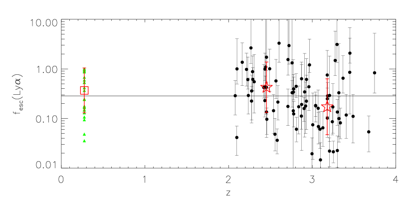
Figure 10: Escape fraction of Ly$\alpha$ photons as a function of redshift for the 83 LAEs in the final sample. The solid horizontal line denotes the median escape fraction of 29%. Also shown is the median escape fraction for the two redshift bins at $1.9<z<2.8$ and $2.8<z<3.8$ (open red stars), with error-bars corresponding to the standard deviation of log($f_{esc}$) within each bin. The escape fractions of LAEs at $z=0.3$ with their median from Atek et al. (2009) (green triangles, red open square) are also displayed.

Measured values of $f_{esc}(Ly\alpha)$ are reported in Table 1. Figure 10 presents the Ly$\alpha$ escape fraction of our LAEs as a function of redshift (black circles). A broad range in the escape fraction (2% to 100%) is observed. LAEs in our sample show a median escape fraction $\tilde{f}_{esc}(Ly\alpha)=0.29\pm 0.04$, and a mean escape fraction $\langle f_{esc}(Ly\alpha)\rangle=0.55\pm 0.08$ (formal error on the mean). All objects showing $f_{esc}(Ly\alpha)>1$ are consistent with $f_{esc}(Ly\alpha)=1$ to 1.5$\sigma$.

A recent study by Hayes et al. (2010a) used a pair of optical and NIR narrow-band filters to sample the Ly$\alpha$ and H$\alpha$ lines over the same volume. By comparing the Ly$\alpha$ and H$\alpha$ luminosities of a sample of 38 LAEs at $z=2.2$, they derived a lower limit of 0.32 for the average Ly$\alpha$ escape fraction of LAEs, a value consistent with our measured average. Another estimation of the Ly$\alpha$ escape fraction was done by Verhamme et al. (2008) using an independent method on their spectroscopic sample of 11 high-$z$ galaxies (8 of which are LAEs). Fitting the Ly$\alpha$ emission line velocity profiles using Monte Carlo radiative transfer simulations yielded best-fit values for $f_{esc}(Ly\alpha)$ between 0.02 and 1, with a median value of 0.17, in good agreement with our observed median value. The agreement between these three independent estimations using a different set of techniques is encouraging.

A median (mean) escape fraction of $\sim 20$% ($\sim 50$%) is one order of magnitude higher than that adopted in the semi-analytical models of Le Delliou et al. (2005), in which a 2% escape fraction combined with a top-heavy IMF is used to match the output of the models to the observed Ly$\alpha$ and UV luminosity function of LAEs at different redshifts. We observe a much larger escape fraction, and our measured $EW$s can be explained by standard stellar populations with normal IMFs. Also, the large scatter seen in Figure 10 implies that using a single value of $f_{esc}(Ly\alpha)$ to model the LAE galaxy population is not a realistic approach.

It is important to remark that estimating the escape fraction directly from the observed $SFR(Ly\alpha)/SFR(UV)$ ratio, by assuming LAEs are dust-free galaxies, would imply a significant overestimation of its value. For example, the best-fit SED to the stacked optical photometry of $z=3.1$ LAEs in Gawiser et al. (2006a), which has $A_{V}=0^{+0.1}_{-0.0}$, implies a best-fit escape fraction of 0.8 (although the uncertainty in the fit allows for a escape fraction $>0.2$, in agreement with our results). Similarly, the ratios measured by Ouchi et al. (2008), Nilsson et al. (2009a), and Guaita et al. (2010) imply escape fractions in the 0.5 to 1.0 range if dust is not considered. As discussed above, if we were to completely neglect dust extinction we, would measure a value of 0.87 for our sample.

5.3 Evolution of the Ly$\alpha$ Escape Fraction in LAEs

No significant evolutionary trend is present across the $1.9<z<3.8$ range of our objects in Figure 10, where the median escape fractions for the two $1.9<z<2.8$ and $2.8<z<3.8$ redshift bins (red open stars in Figure 10) are consistent with the median for the whole sample. In order to investigate if the Ly$\alpha$ escape fraction of LAEs evolves over a larger baseline in cosmic time, we also show results found in the literature at a lower redshift. At higher redshifts the Ly$\alpha$ escape fraction for LAEs remains poorly constrained, although attempts to measure it exist in the literature (eg. Ono et al., 2010)

At low redshift Atek et al. (2009) performed optical spectroscopy on a sample of $z\simeq 0.3$ LAEs (Deharveng et al., 2008) and used the H$\alpha$ luminosity, in combination with dust extinctions derived from the Balmer decrement, to estimate the Ly$\alpha$ escape fraction of these objects. A similar range in the escape fraction is observed for $z\simeq 0.3$ and $2<z<4$ LAEs, with the former showing values ranging from 0.03 to 1, implying that there has not been significant evolution in $f_{esc}(Ly\alpha)$ over the $\sim$8 Gyr from $z\sim 3$ to $z\sim 0.3$. At very high redshifts ($z=5.7$ and 6.6) Ono et al. (2010) has estimated the Ly$\alpha$ escape fraction of a sample of a few hundred narrow-band selected LAEs using a similar method to the one used here, except that their intrinsic $SFRs$ were measured by SED fitting. Their escape fractions are consistent with our measured values at $2<z<4$, although their error-bars are large. Therefore we detect no significant evolution in $f_{esc}(Ly\alpha)$ over the $0.3<z<6.6$ range.

This lack of evolution in the Ly$\alpha$ escape fraction of LAEs must be interpreted with caution, since nothing ensures that the LAE selection technique recovers the same galaxy populations at these very distant epochs in the universe. Furthermore, since the selection is based on the strength of the Ly$\alpha$ line relative to the the underlying continuum (i.e. the $EW$ of the line), the technique will tend to favor galaxies with high Ly$\alpha$ escape fractions, as long as they satisfy the brightness cut of the survey, at any redshift. Therefore, the lack of evolution in $f_{esc}(Ly\alpha)$ cannot be interpreted as constancy in the physical conditions in the ISM of these galaxies. For example, while at low redshift the escape fraction is most likely dominated by dust absorption, at $z\sim 6$ it is most likely dominated by IGM attenuation.

5.4 The Relation between $f_{esc}$(Ly$\alpha$) and Dust

As discussed in §1, a major subject of debate regarding the escape of Ly$\alpha$ photons from star-forming galaxies is the role played by dust. It is not clear whether the resonant nature of the transition produces Ly$\alpha$ photons to be extincted more, less, or in the same amount as continuum photons outside the resonance. For example, while Ly$\alpha$ photons should originate in the same regions as H$\alpha$ photons, we have no reason to expect the extinction seen by Ly$\alpha$ photons to follow the nebular extinction relation $E(B-V)_{stars}=0.44E(B-V)_{gas}$ seen for non-resonant hydrogen transitions in star-forming galaxies at $z=0$ (Calzetti, 1997), since resonant scatter makes the optical paths seen by Ly$\alpha$ completely different from the one seen by other lines like H$\alpha$ or H$\beta$. Furthermore, it has not been established if the above relation holds at high redshift or not.

In order to test this issue we parameterize the ratio between the dust opacity seen by Ly$\alpha$ and that which continuum photons at the same wavelength would see in the absence of the transition. Following Finkelstein et al. (2008), we adopt the parameter $q=\tau_{Ly\alpha}/\tau_{\lambda=1216}$, where $\tau_{\lambda}=k_{\lambda}E(B-V)/1.086$ and $k_{\lambda}$ is assumed to be a Calzetti et al. (2000) dust attenuation law. $E(B-V)$ is always taken to be the stellar color excess derived from the UV slope.

A value of $q\sim 0$ implies that Ly$\alpha$ photons suffer very little extinction by dust, as is expected in an extremely clumpy multi-phase ISM. Large values ($q\gg 1$) represent cases in which scattering of Ly$\alpha$ photons introduces a strong increase in the dust attenuation as is expected in a more homogeneous ISM. As discussed in §1, not only the structure of the ISM determines the value of $q$, but also the kinematics of the ISM, since favorable configurations (eg. an expanding shell of neutral gas which allows backscattering) can reduce the amount of dust extinction seen by Ly$\alpha$ photons. All these processes are coupled in determining the value of $q$, and discriminating between them requires a joint analysis of the UV, Ly$\alpha$, and H$\alpha$ luminosities, the dust extinction either from the shape of the UV continuum or from Balmer decrements, and the profiles of the latter two emission lines. Until such data exist, interpretation is difficult, but we can still gain insights about the escape of Ly$\alpha$ photons and the dust properties of LAEs from the measured value of $q$.

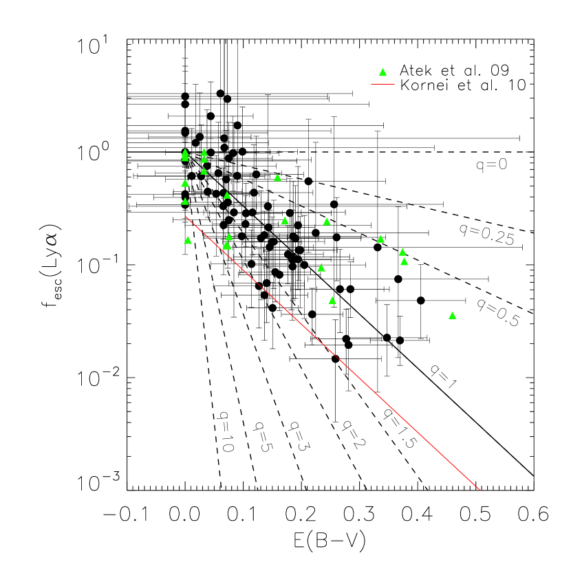
Figure 11: Ly$\alpha$ escape fraction as a function of E(B-V). Dashed lines show the expected correlation for different values of the parameter $q=\tau_{Ly\alpha}/\tau_{\lambda=1216}$. The red line displays the relation for LBGs showing Ly$\alpha$ in emmission from Kornei et al. (2010). Green triangles show the values for $z\simeq 0.3$ LAEs from Atek et al. (2009).

In Figure 11 we present the Ly$\alpha$ escape fraction versus the dust reddening $E(B-V)$ for our sample of LAEs. A clear correlation between the escape fraction and the amount of dust extinction is seen. Also shown are the expected correlations for different values of the parameter $q$. The LAE population falls along the $q=1$ relation. The median for the whole sample is $\tilde{q}=0.99\pm 0.44$ (median absolute deviation error), implying that in most LAEs the Ly$\alpha$ emission suffers a very similar amount of dust extinction to that experienced by UV continuum light.

Our results show good agreement with those of Hayes et al. (2010a). In their work, 5 out of 6 LAEs at $z=2.2$ detected in both Ly$\alpha$ and H$\alpha$ show escape fractions and dust reddenings consistent with the $q=1$ relation. The same is true for the large majority of their LAEs with no H$\alpha$ detections for which they could only provide lower limits to the escape fraction. Our LAEs at $2<z<4$ also occupy the same region in the $E(B-V)$ vs. $f_{esc}(Ly\alpha)$ plane as the low redshift LAEs ($z\simeq 0.3$ Atek et al., 2009) shown as green triangles in Figure 11. This implies that not only the Ly$\alpha$ escape fraction in LAEs does not evolve with redshift as shown in §5.3, but its dependence on the dust content of the ISM remains the same from $z=4$ to 0.3.

The LAE selection criteria imply that these objects are chosen to be the galaxies with the largest Ly$\alpha$ escape fractions given their Ly$\alpha$ luminosities and dust content at any redshift. Most likely, a combination of ISM geometry and kinematics favors the escape of Ly$\alpha$ photons in these galaxies as compared to the common galaxy population at any redshift. Hence, when examining Figure 11 we should think of LAEs as the upper envelope of the escape fraction distribution at any E(B-V). For example, Kornei et al. (2010) found that LBGs with Ly$\alpha$ emission typically lie below the $q=1$ relation. In their work they parameterized the difference in the extinction seen by Ly$\alpha$ and continuum photons by the “relative escape fraction”, $f_{esc,rel}$, which relates to $q$ by the following relation

$$q=\frac{log(f_{esc,rel})}{0.4k_{\lambda=1216}E(B-V)}$$ (4)

They find LBGs to have $\langle f_{esc,rel}\rangle=0.27$ (which does not include LBGs showing Ly$\alpha$ in absorption). We present this relation for LBGs as a red line in Figure 11. This finding supports our previous point, namely that LAEs are the upper envelope to the overall galaxy population in the $E(B-V)$ vs. $f_{esc}(Ly\alpha)$ plane.

Our result should not be interpreted as evidence against the existence of a clumpy multiphase ISM in LAEs, since in the presence of a completely homogeneous ISM we expect $q>1$. Nevertheless, our result indicates that either a clumpy ISM, a favorable kinematic configuration of the ISM, or a combination of both, can reduce the amount of dust seen by scattering Ly$\alpha$ photons only up to the point where they encounter the same level of dust opacity as the continuum. Since LAEs by definition will be the galaxies with the largest Ly$\alpha$ escape fractions at any value of $E(B-V)$, the absence of a significant number of points at low values of $q$ in Figure 11 suggests that enhancement of the Ly$\alpha$ $EW$s due to clumpiness in the ISM is not a common process in galaxies.

6 The Ly$\alpha$ Luminosity Function

It has been well established in the literature that the Ly$\alpha$ luminosity function does not show significant evolution from $z=3$ to 6 (Shimasaku et al., 2006; Tapken et al., 2006; Ouchi et al., 2008). On the other hand, a strong decrease of roughly one order of magnitude is seen in the abundance of LAEs from $z\sim 3$ down to $z\sim 0.3$ (Deharveng et al., 2008). At what point in cosmic time this decrease starts to take place, and how well it traces the $SFR$ history of the universe, is unknown. Recently there have been reports of possible evolution in the number density of LAEs between $z\sim 3$ and $z\sim 2$ (Nilsson et al., 2009a), but, as stated by the same authors, these results might be affected by cosmic sample variance over the surveyed volumes. Furthermore, Cassata et al. (2011) find no evolution in the luminosity function across these epochs in their sample of spectroscopically detected LAEs. The existence of evolution in the luminosity function (or number density) of LAEs down to these lower redshifts is still a subject of debate.

By examining the redshift distribution of our LAEs (Figure 2), we found indications that their number density might be decreasing towards lower redshifts ($z<3$) in our sample (§3). In this section we measure the Ly$\alpha$ luminosity function of LAEs, and study any potential evolution down to $z\sim 2$. We restrict the measurement of the luminosity function to LAEs in the COSMOS and GOODS-N fields, which account for 81% (80/99) of the total sample. Both MUNICS and XMM-LSS lack deep X-ray data comparable to the one available in COSMOS and GOODS-N, so it is not possible to identify AGNs in those fields.

6.1 Measurement of the Luminosity Function

To measure the luminosity function we adopt a $1/V_{max}$ formalism similar to the one used by Cassata et al. (2011). We compute the volume density of objects in bins of $\Delta log(L)=0.125$ dex, as the sum of the inverse of the maximum volumes over which each object in the luminosity bin could have been detected in our survey. As discussed in §3, the depth of the observations is variable across the surveyed area. The whole survey covers 169 arcmin², corresponding to 60 VIRUS-P pointings. Each pointing was covered by six dithered observations, which accounts for 360 independent observations each reaching different depths. The noise spectrum for each IFU fiber in each of these observations is an output of our data processing pipeline, and can be directly translated into an effective line luminosity limit for Ly$\alpha$ at each redshift (see Figure 1).

For each object, $V_{max}$ is given by

$$V_{max}=\displaystyle\sum_{i}V_{max,i}$$ (5)

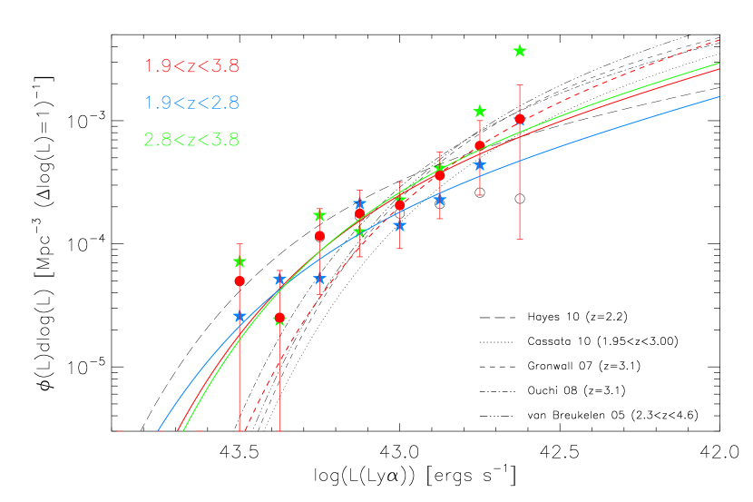
Figure 12: Ly$\alpha$ luminosity function of the HETDEX Pilot Survey sample of 80 LAEs in COSMOS and HDF-N, shown before and after applying the completeness correction (open black and filled red circles respectively). Poisson error-bars are included. Also displayed are the completeness corrected luminosity function for the two redshift bins at $1.9<z<2.8$ and $2.8<z<3.8$ (blue and green stars respectively), and the luminosity functions of van Breukelen et al. (2005); Gronwall et al. (2007); Ouchi et al. (2008); Hayes et al. (2010a),and Cassata et al. (2011). Schechter fits to the full sample, as well as the low-z and high-z samples, are also presented (solid red, blue, and green curves respectively). The red dashed line denotes the best Schechter fit to the $L(Ly\alpha)\leq 10^{43}$erg s^-1 bins.

where $V_{max,i}$ is the integral of the co-moving volume over all the redshifts at which the object could have been detected (i.e. where the luminosity limit is lower than the objects luminosity) for each observation $i$. Summing over the inverse of $V_{max}$ for all objects in each luminosity bin then yields the luminosity function shown as open black circles in Figure 12.

As mentioned briefly in §3 and discussed extensively in Paper I, the effects of incompleteness are important over all luminosities in our survey. Completeness is a direct function of the S/N at which the emission line is detected in our spectra. Since the limiting luminosity is not constant at all redshifts (Figure 1), objects of the same luminosity can be detected with high significance, and hence high completeness, at certain redshifts and with low significance and low completeness at others. This is different than, for example, imaging surveys where objects are detected in a narrow redshift range, and the S/N is close to a unique function of the luminosity. In those cases, incompleteness becomes only important in low luminosity bins, where the objects flux approach the depth of the images. In our case, we must account for incompleteness over the whole luminosity range if we want to get a proper estimate of the luminosity function.

In Paper I we present a detailed completeness analysis of our survey based on simulations of the recovery fraction of synthetic emission lines at different S/N in our spectra. Using these recovery fractions we correct the observed Ly$\alpha$ luminosity function calculated as described above. The resulting completeness-corrected luminosity function is shown by the red filled circles in Figure 12. Error-bars shows Poisson uncertainties only, and correspond to a lower limit for the error since they do not include cosmic variance, although Ouchi et al. (2008) show that for volumes such as the one surveyed here ($\sim 10^{6}$ Mpc³), cosmic sample variance uncertainties are not significantly higher than Poisson errors.

We fit the observed Ly$\alpha$ luminosity function using a Schechter (1976) function of the following form

$$\phi(L)dL=\phi^{*}(L/L^{*})^{\alpha}\;exp(-L/L^{*})\;d(L/L^{*})$$ (6)

Since the depth of our observations ($\sim 5\times 10^{-17}$ erg s^-1cm^-2 in line flux) is somewhat limited, we do not consider our data to be sufficiently deep to constrain the faint-end slope ($\alpha$) of the luminosity function. We consider the best available constraint on $\alpha$ to come from the spectroscopic survey recently performed by Cassata et al. (2011). They measure $\alpha\simeq-1.7$ using a survey which reaches more than one order of magnitude deeper than ours in terms of limiting line flux ($\sim 1.5\times 10^{-18}$ erg s^-1cm^-2). We take their measured $\alpha$ as our fixed fiducial value for the faint-end slope of the luminosity function, but also report results assuming $\alpha=-1.5$, since that is the value most commonly used in the literature (Gronwall et al., 2007; Ouchi et al., 2008). Our results do not depend significantly on the assumed value of $\alpha$.

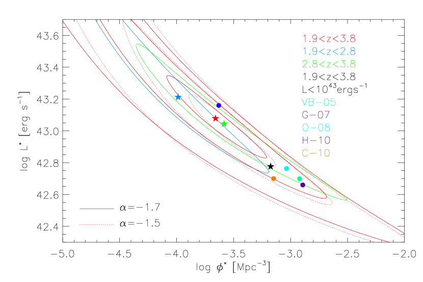
Figure 13: Contours show 1, 2, and 3$\sigma$ confidence limits for the luminosity function parameters $L^{*}$ and $\phi^{*}$. Stars show our results for the full sample and the two redshift bins at $1.9<z<2.8$ and $2.8<z<3.8$. The parameters estimated by van Breukelen et al. (2005); Gronwall et al. (2007); Ouchi et al. (2008); Hayes et al. (2010a), and Cassata et al. (2011) are also presented (filled circles).

The best-fit Schechter luminosity function ($\alpha=-1.7$) is shown by the solid red line in Figure 12, and 1, 2, and 3$\sigma$ confidence limits for the parameters are shown in Figure 13. The best fit parameters for $\alpha=-1.7$ and -1.5 are reported in the first two rows of Table 2.

6.2 Comparison with Previous Measurements

Figure 12 also shows the Ly$\alpha$ luminosity functions measured by several authors at similar redshifts. The overall agreement with previous measurements is good. The Ly$\alpha$ luminosity functions of van Breukelen et al. (2005); Gronwall et al. (2007); Ouchi et al. (2008); Hayes et al. (2010a), and Cassata et al. (2011) measured at $2.3<z<4.6$, $z=3.1$, $z=3.1$, $z=2.2$, and $1.95<z<3$ respectively, agree with our observed values to within $\sim 1\sigma$ (Poisson) at all luminosities. The Hayes et al. (2010a) measurement shows better agreement with our data at the bright end of the luminosity function. This is in fact surprising, as their measurement was performed over a smaller volume ($5.4\times 10^{3}$ Mpc³) and a fainter range in luminosities ($2\times 10^{41}-5\times 10^{42}$ erg s^-1) than the other mentioned works.

Our best-fit Schechter function appears to be flatter than previous measurements over a similar range in luminosities. Figure 13 shows that this difference is because we derive a higher $L^{*}$ and a lower $\phi^{*}$ than previous authors (except Hayes et al. (2010a) who found a very similar value for $\phi^{*}$ but a larger value for $L^{*}$). The best-fit parameters measured by van Breukelen et al. (2005); Gronwall et al. (2007); Ouchi et al. (2008); Hayes et al. (2010a), and Cassata et al. (2011) fall within our 2$\sigma$ confidence contour. This last work is the only one of the mentioned luminosity function measurements in which $\alpha=-1.7$. For all the other measurements, the faint-end slope was either assumed or measured to be $-1.5$ except for van Breukelen et al. (2005) who used $-1.6$. For better comparison, Figure 13 also shows uncertainty contours for our fit assuming $\alpha=-1.5$ (dotted contours). As mentioned above, the value of $\alpha$ does not change our results in any significant way.

The $L^{*}$ and $\phi^{*}$ parameters are strongly correlated with each other, so the $2\sigma$ discrepancy with previous measurements is not surprising as it follows the sense of the correlation. Most importantly, we survey a very large volume and hence are able to find rare high luminosity objects. The luminosity functions derived in these studies typically stop at $\sim 10^{43}$ erg s^-1, while we find objects up to three times brighter luminosities. If we fit a Schechter function to only bins with $L(Ly\alpha)\leq 10^{43}$ erg s^-1, we obtain the luminosity function shown as a dashed red line in Figure 12, which is in much better agreement with previous measurements (black star in Figure 13 and third row in Table 2).

6.3 Evolution of the Ly$\alpha$ Luminosity Function

As mentioned above, evidence suggests that the Ly$\alpha$ luminosity function does not significantly evolve between $z\sim 3$ and $z\sim 6$. While at the high end of this redshift range ($z\gtrsim$5) IGM absorption might become important and the lack of evolution might imply an increase in the intrinsic Ly$\alpha$ luminosity function (Cassata et al., 2011), at least between $z\sim 4$ and $z\sim 3$ the lack of intrinsic evolution seems well supported as changes in IGM transmission are negligible (Ouchi et al., 2008). We can extend these studies to lower redshifts and ask: Does the luminosity function show any significant evolution down to $z\sim 2$?

To test for possible evolution, we have again divided our sample in the two redshift bins defined in §4, one at low-redshift ($1.9<z<2.8$), and another one at high-redshift ($2.8<z<3.8$). We measure the luminosity function in each of these bins independently. The results are shown in Figure 12, best fit parameters are presented in Table 2, and 1$\sigma$ confidence limits are shown in Figure 13. At $L(Ly\alpha)\leq 10^{43}$ erg s^-1, where cosmic variance is lower than at higher luminosities, the low-$z$ luminosity function seems to be systematically lower than the high-$z$ luminosity function by a factor about $\sim 2$, in agreement with what we observed in §3 when comparing the redshift distribution of our objects to the predictions for a non evolving luminosity function. Still, both the high-$z$ and low-$z$ luminosity functions fall within their mutual Poisson uncertainties, and there is overlap between the 1$\sigma$ confidence limits in their best-fit Schechter parameters (Figure 13).

We conclude that we find indications for evolution in the luminosity function over the $2\lesssim z\lesssim 4$ range, with a decrease towards lower redshifts, but only at a low significance level. Larger samples, such as the ones HETDEX will produce in its few firsts months of operation, will be required to confirm this. If real, this evolution implies that the large drop in the Ly$\alpha$ luminosity function, evident at $z\simeq 0.3$, starts to occur at $z>2$. Another way of searching for evolution in the Ly$\alpha$ luminosity function is to integrate it, and compare the implied Ly$\alpha$ luminosity density at each redshift. This is the subject of the next section.

7 Evolution of the Ly$\alpha$ Luminosity Density and the Global Escape Fraction of Ly$\alpha$ Photons.

In §5.2 we measured the median escape fraction of Ly$\alpha$ photons at $2<z<4$ in LAEs to be $\sim 30$%. This does not represent the median escape fraction of the whole galaxy population at those redshifts, since LAEs will, by definition, be biased towards having high $f_{esc}(Ly\alpha)$. On the other hand, we can integrate the Ly$\alpha$ luminosity function measured in the previous section to estimate the Ly$\alpha$ luminosity density ($\rho_{Ly\alpha}$) at these redshifts. Comparing this observed luminosity density with that predicted from the global $SFR$ density ($\rho_{SFR}$) for the entire galaxy population provides an estimate of the global escape fraction of Ly$\alpha$ photons and its evolution with redshift. The above approach is equivalent to taking the ratio between the $SFR$ density implied by the observed Ly$\alpha$ luminosity density using Equation 2 ($\rho_{SFR,Ly\alpha}$), and the total $\rho_{SFR}$. This method has been applied by Cassata et al. (2011). In this work we extend their analysis which included the Cassata et al. (2011) data at $2<z<6.6$, the measurement of Gronwall et al. (2007) at $z=3.1$, and the data of Ouchi et al. (2008) at $z=3.1$, 3.7, and 5.7. We add the HETDEX Pilot Survey data points at $1.9<z<3.8$, as well as the $z\sim 0.3$ LAE data from Deharveng et al. (2008) and Cowie et al. (2010), the $z=2.2$ data of Hayes et al. (2010a), the $z=4.5$ measurement by Dawson et al. (2007), the measurement at $z=5.7$ of Shimasaku et al. (2006), the $z=6.5$ data from Kashikawa et al. (2006), the data of Ouchi et al. (2010) at z=6.6, and the $z=7.7$ measurement of Hibon et al. (2010). A similar dataset has been analyzed in this way in a recent submission by Hayes et al. (2010b), although using a different set of H$\alpha$ and UV luminosity functions at different redshifts to estimate the total SFR density.

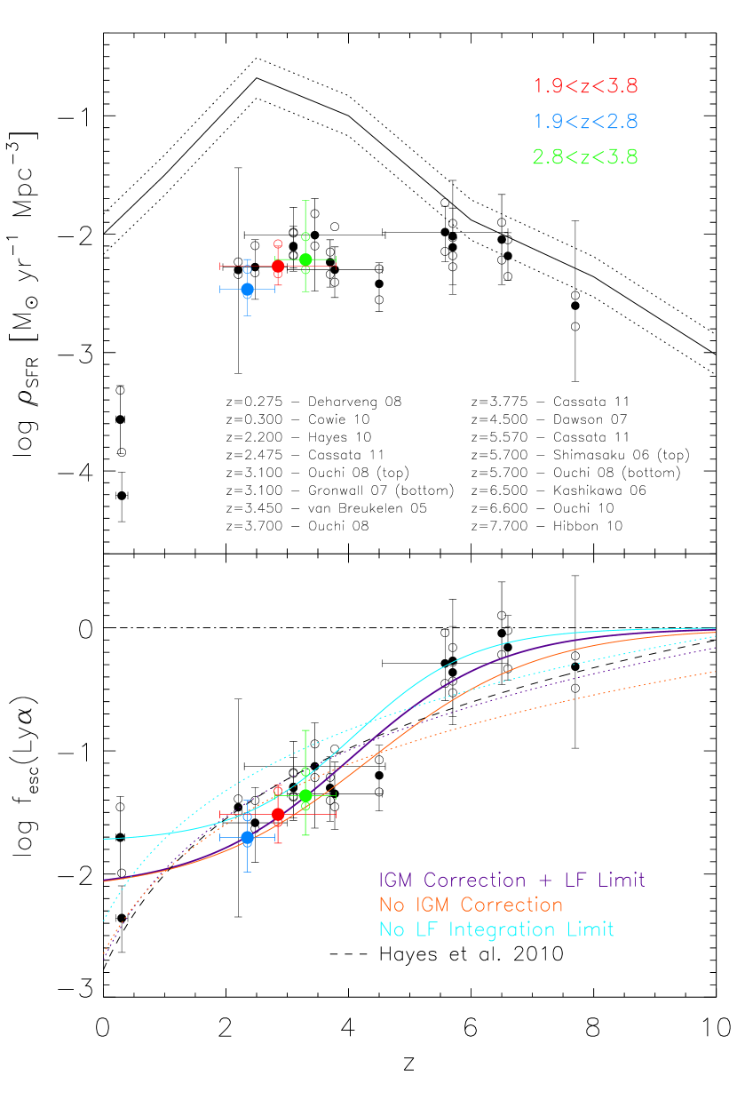
Figure 14: Top panel: $SFR$ density ($\rho_{SFR}$) as a function of redshift. The solid and dotted lines show the total $\rho_{SFR}$ from Bouwens et al. (2010b) and its typical uncertainty of 0.17 dex. Blue, green, and red filled circles show $\rho_{SFR,Ly\alpha}$ derived from the Ly$\alpha$ luminosity function in the two redshift bins at $1.9<z<2.8$ and $2.8<z<3.8$, as well as for the full sample. Black filled circles show the derived densities at different redshifts from the luminosity functions of van Breukelen et al. (2005); Shimasaku et al. (2006); Kashikawa et al. (2006); Gronwall et al. (2007); Dawson et al. (2007); Ouchi et al. (2008); Deharveng et al. (2008); Ouchi et al. (2010); Cowie et al. (2010); Hayes et al. (2010a); Hibon et al. (2010), and Cassata et al. (2011). Raw values computed without applying an IGM correction are shown by the open circles below each measurement. Values computed integrating the Ly$\alpha$ luminosity functions all the way down to $L(Ly\alpha)=0$ are shown by the open circles above each measurement. Bottom panel: Escape fraction of Ly$\alpha$ photons for the overall galaxy population, derived from the ratio between the Ly$\alpha$ derived $\rho_{SFR,Ly\alpha}$ and the total value at each redshift. The dashed line marks an escape fraction of 100%. Solid lines shows our best fit to the data given by Equation 6, while dotted lines show the best fit powerlaw functions. Purple, orange, and cyan colors indicate fits to the escape fraction measurements including an IGM correction and an integration limit for the luminosity function, ignoring the IGM correction, and ignoring the luminosity function integration limit respectively. The black dashed line shows the result of Hayes et al. (2010b).

The top panel in Figure 14 shows $\rho_{SFR,Ly\alpha}$ derived from the observed Ly$\alpha$ luminosity density using Equation 2. We present our results for the full sample and for the low-$z$ and high-$z$ bins of the HETDEX Pilot Survey (red, blue, and green filled circles), as well as the compilation of data points calculated from the Ly$\alpha$ luminosity functions at $0.3<z<7.7$ mentioned above (black filled circles). Vertical error-bars are estimated from the published uncertainties in $L^{*}$ and $\phi^{*}$, and horizontal error-bars show the redshift range of the different samples (omitted for narrow-band surveys). Also presented is the latest estimate of the total $SFR$ density history of the universe from Bouwens et al. (2010b), which has been derived from the best to date collection of dust extinction corrected UV luminosity functions at a series of redshifts between 0 and 8, and shows a typical uncertainty of 0.17 dex (Bouwens et al., 2010b, and reference therein).

A source of systematic error in measuring the Ly$\alpha$ luminosity density comes from the choice of the luminosity limit down to which the integration of the luminosity function is performed. An excellent discussion on this issue can be found in Hayes et al. (2010b). With the goal of estimating the volumetric Ly$\alpha$ escape fraction by comparison to the UV derived SFR density, we should ideally choose an integration limit consistent with the one used by Bouwens et al. (2010b) to integrate their UV luminosity functions. In this way we can ensure both measurements are roughly tracing the same galaxies. In the case of Ly$\alpha$ and UV luminosity functions this is nontrivial, as the exact number will depend on the, mostly unconstrained, shape of the Ly$\alpha$ escape fraction distribution for galaxies as a function UV luminosity. In lack of a better choice, we follow the approach of Hayes et al. (2010b), and integrate the Ly$\alpha$ luminosity functions down to the same fraction of $L^{*}$ as the UV luminosity function were integrated (0.06$L_{z=3}^{*}$ in the case of Bouwens et al. (2010b)). For consistency with Hayes et al. (2010b), and in order to allow for a better comparison with their results, we define this limit using the Gronwall et al. (2007) luminosity function at $z=3.1$, for which the integration limit becomes $0.06L_{G07}^{*}=2.66\times 10^{41}$ erg s^-1. For all the data points in Figure 14 we also shows the same measurements obtained by integrating the luminosity functions down to zero luminosity (upper open circles). The unlimited integration typically overestimates the luminosity (SFR) density by $\sim 60$%. This provides a notion of the maximum impact that the choice of this integration limit has on the measured value of the luminosity density.

A second source of systematic error in the above measurement comes from the role that IGM scattering has at reducing the observed Ly$\alpha$ flux of sources at very high redshifts. Although all our previous analysis neglected the effects of IGM scattering on the Ly$\alpha$ line, this approach was only well justified at our redshifts of interest ($z<4$), where IGM scattering is negligible for our purposes (see discussion in §1 and §5). To study the escape of Ly$\alpha$ photons from galaxies across a larger redshift range, we should try to incorporate the effect of the IGM, which is not negligible for the measurements at very high redshift ($z\sim 6$). As discussed in §1, the effects of the ISM and IGM kinematics in and around galaxies makes this correction very difficult (Dijkstra et al., 2007; Verhamme et al., 2008). To first order, we have applied a correction using the Madau (1995) average Ly$\alpha$ forest opacity, and assuming that only half of the Ly$\alpha$ line flux suffers this attenuation. The filled symbols in Figure 14 include this correction. Raw measurements done without applying this correction are also shown in Figure 14 as the open circles below each data point. While this correction can become large ($\sim 50$%) at the highest redshifts, it impact is still within the 1$\sigma$ uncertainties coming from the luminosity function measurements.

In accordance with the low significance hint of evolution presented in §6.3, in the $2<z<4$ range, all the estimates of $\rho_{SFR,Ly\alpha}$ agree with each other within 1$\sigma$. However, by examining the overall trend of the data points, and keeping in mind the ones at higher and lower redshifts, there are clearly indications for evolution in the $SFR$ density derived from Ly$\alpha$ from $z\sim 7$ down to $z\sim 0.3$, with a steady decrease towards lower redshifts across the $2<z<4$ range. Although the uncertainties in the $2<z<4$ range are large, allowing any two datapoints to be consistent with each other, the overall trend implies a decrease in $\rho_{Ly\alpha}$ of roughly a factor of $\sim 2$ from $z=4$ to 2. We stress the need for larger samples of LAEs at these redshifts to better constrain this evolution.

The bottom panel of Figure 14 shows the global average escape fraction of Ly$\alpha$ photons, which is given by the ratio between $\rho_{SFR,Ly\alpha}$ and $\rho_{SFR}$ at any given redshift. The average escape fraction derived from our Ly$\alpha$ luminosity function over the whole $1.9<z<3.8$ range is ($3.0^{+2.3}_{-1.2}$)%. Errors include 1$\sigma$ uncertainties in the luminosity function parameters and the 0.17 dex uncertainty in the total SFR density from Bouwens et al. (2010b). For our $1.9<z<2.8$ and $2.8<z<3.8$ bins we derived a mean Ly$\alpha$ escape fraction for the overall galaxy population of $(2.0^{+2.0}_{-0.9})$% and $(4.3^{+10.3}_{-2.2})$% respectively. This amount of evolution is not statistically significant, but we believe it to be real in the context of the overall trend seen in Figure 14. It also does not contradict the lack of evolution in the escape fraction for LAEs observed in §5.2, since, as mentioned above, the LAE selection tends to identify galaxies with high $f_{esc}(Ly\alpha)$ at any redshift, independent of the value of the escape fraction of the total galaxy population. The median dust extinction of a factor of $\sim 3$ measured in §4.2 implies that LAEs contribute roughly 10% of the total star formation at $2<z<4$. This contribution rises to 80% by $z\sim 6$, implying that galaxies at these redshifts must have very low amounts of dust in their ISM, which is consistent with the very blue UV slopes of continuum selected galaxies at these high redshifts (Bouwens et al., 2010a; Finkelstein et al., 2010). The observed behavior is also consistent with the results of Stark et al. (2010), who find the fraction of LBGs showing high $EW$ Ly$\alpha$ emission to roughly double from $z=4$ to 6. A similar result was also reported by Ouchi et al. (2008), who measure a significant level of evolution in the UV luminosity function between their $z=3.7$ and $z=6.6$ samples of LAEs, which was not traced by the Ly$\alpha$ luminosity function.

The above escape fractions are in agreement with the result of Hayes et al. (2010a), who measured an overall Ly$\alpha$ escape fraction of $(5.3\pm 3.8)$% at $z=2.2$ by comparing the Ly$\alpha$ and H$\alpha$ luminosity function of narrow-band selected emission line galaxies over the same co-moving volume. On the other hand, by applying the same method used here Cassata et al. (2011) measured an average escape fraction of $\sim$20% at $z=2.5$. The difference is easily explained by the fact that the latter authors compared their observed Ly$\alpha$ derived $SFR$ density (which agrees with our value) to the total $SFR$ density uncorrected by dust, which underestimates the true value at these redshifts.

It is evident that a strong decrease in the Ly$\alpha$ escape fraction of galaxies occurred between $z\sim 6$, and $z\sim 2$. In order to quantify this decrease we fit the data points in the lower panel of Figure 14 using two different functional forms. First, we fit a power-law of the form

$${\rm log}(f_{esc}(z))={\rm log}(f_{esc}(0))+\xi\;{\rm log}(1+z)$$ (7)

This is the same parametrization used by Hayes et al. (2010b) to fit the history of the global Ly$\alpha$ escape fraction. Best fit parameters are presented in Table 3. In order to provide a quantitative assessment of the impact of systematic errors in the measurement, we not only fit our best estimates of the escape fraction at each redshift, but also the values calculated ignoring the luminosity function integration limit, and the IGM correction. The best fitting power-laws for these three sets of data points are shown as dotted lines in Figure 14. For comparison with the results of Hayes et al. (2010b), we should consider our raw measurement without including the effects of the IGM, as a correction of this type was not done in their work. They find best fit values of ${\rm log}(f_{esc}(0))=-2.8\pm 0.1$, and $\xi=2.6\pm 0.2$, in excellent agreement with our result.

While the power-law model provides a reasonable fit to the data, it seems to systematically overestimate the measured values of $f_{esc}(Ly\alpha)$ in the $2<z<5$ range, and underestimate them in the $5<z<8$ range. The data points in Figure 14 seem to indicate a sudden drop, or transition in the escape fraction between $z=6$ and 2. A similar transition, in a coincident redshift range, is observed in the dust extinction derived from the UV slope of continuum selected galaxies (Bouwens et al., 2009). Given the important role that dust has at regulating the escape of Ly$\alpha$ photons, it would not be surprising if the dust content and the Ly$\alpha$ escape fraction of galaxies present a similar evolution with redshift. In order to quantify this behavior we also fit a transition model of the following form,

$${\rm log}(f_{esc}(z))=\frac{{\rm log}(f_{esc}(0))}{2}\;(1-{\rm tanh}(\theta(z-z_{tr}))$$ (8)

where $z_{tr}$ is the transition redshift at which the decrease in the escape fraction takes place ($f_{esc}=1$ for $z\gg z_{tr}$), and the parameter $\theta$ determines the sharpness of the transition. Best-fit parameters to the measured escape fraction at each redshift, and the values without IGM correction, and without a luminosity function integration limit are presented in Table 3. Our best-fit transition model, implies a very high Ly$\alpha$ escape fraction of $\sim 80$% at $z\sim 6$, which drops softly from $z\sim 6$ to $z\sim 2$, with a characteristic transition redshift at $z_{tr}=4.0\pm 0.5$, in order to reach a value of $\sim 1$% in the local universe.

By analyzing the values in Table 3, It can be seen that, given the current uncertainties, the IGM correction and the choice of the luminosity function integration limit do not induce major changes in the best-fit parameters, especially in the case of the power-law exponent. The largest effect is that of the integration limit on the escape fraction at $z=0$. The reason for this is that low $L^{*}$ values are measured for the Ly$\alpha$ luminosity functions at low redshift. Therefore, the integration limit lays closer to $L^{*}$ at these redshifts, making the value of the luminosity density more dependent on it.

Equation 8 predicts the average Ly$\alpha$ luminosity of star-forming galaxies at any redshift given their average $SFR$, and it might prove useful for semi-analytic models of galaxy formation attempting to reproduce the Ly$\alpha$ luminosity function. However, the escape fraction shows a very large scatter for single objects, and it might be systematically different for galaxy populations selected using different methods. Therefore, this relation should be used with caution, and only in an statistical manner. Also, this equation is only valid over the redshift range in which observations are available, and to the extent that current uncertainties allow. For example, given the current uncertainties, we do not consider the escape fraction to be properly constrained at $z>6.6$. While it is tempting to interpret the slight drop seen in the last data point at $z=7.7$ as a possible reduction in Ly$\alpha$ transmission due to the neutralization of the IGM as we walk into the end of re-ionization, the error-bars are too large to allow for any significant conclusions.

8 Conclusions

For a sample of LAEs at $1.9<z<3.8$, detected by means of blind integral field spectroscopy of blank extragalactic fields having deep broad-band optical imaging, we were able to measure the basic quantities $SFR$, $E(B-V)$, UV luminosity, Ly$\alpha$ $EW$, and $f_{esc}(Ly\alpha)$. From these quantities and the correlations observed between them we conclude:

• Over the $2<z<4$ range LAEs show no evolution in the average dust content of their ISM, parameterized by the dust reddening $E(B-V)$, and measured from the UV continuum slope. These objects show a mean $\langle E(B-V)\rangle=0.13\pm 0.01$, implying that dust absorbs $\sim 70$% of the UV photons produced in these galaxies. While one third of LAEs down to our luminosity limit are consistent with being dust-free, the level of dust extinction measured for the rest of the sample is significant, and should not be neglected.

• At $z<3$, we see the possible appearance of a rare (6/89 objects) population of highly reddened ($E(B-V)>0.45$) LAEs, typically showing high Ly$\alpha$ $EW$s. Two of these objects are in the MUNICS field where we do not have deep X-ray data to reject AGNs from our sample. The remaining four objects show low association probabilities ($\leq 0.6$) with their broad-band counterparts, casting doubt on the validity of our UV slope and $EW$ measurements. The presence of these objects in the sample does not affect significantly the average dust properties of LAEs at the low redshift end of our range. If real, these objects are of great interest since their presence could indicate that the fraction of dusty LAEs grows towards lower redshifts. Followup of these objects is necessary to confirm this.

• The Ly$\alpha$ $EW$s of LAEs in our sample are consistent with the expectations for normal stellar populations with metallicities within 1/50 $Z_{\odot}$ and solar. We do not find it necessary to invoke a top-heavy IMF, the presence of population III stars, or an enhancement of the $EW$ due to a clumpy dust distribution in a multi-phase ISM, to explain the observed $EW$s.

• LAEs in our sample show a median uncorrected UV derived $SFR\simeq 11$ M_⊙yr^-1. Correcting the UV luminosities for dust extinction increases this median value to $SFR\simeq 34$ M_⊙yr^-1, implying that assuming LAEs to be dust-free galaxies can translate into large underestimates of their $SFR$s. The ratio between the observed (i.e. uncorrected for dust) UV and Ly$\alpha$ derived $SFRs$ shows a median value of 0.83. Neither this ratio, nor the Ly$\alpha$ $EW$, show significant evolution with redshift across the $2<z<4$ range. These two quantities also show no dependence with $E(B-V)$, implying that the ratio between the amount of dust extinction seen by Ly$\alpha$ photons and that seen by UV photons is independent of the dust-content of the galaxies’ ISM. This finding is at odds with the expectation of models in which a clumpy distribution of dust in a multi-phase ISM promotes the escape of Ly$\alpha$ photons over that of UV continuum photons. It also implies that some combination of ISM geometry and kinematics reduces the amount of extinction seen by Ly$\alpha$ photons from that expected in a static and homogeneous ISM, but only up to the point where it is similar to that experienced by continuum photons.

• The escape fraction of Ly$\alpha$ photons from LAEs, given by the ratio between the observed Ly$\alpha$ luminosity and that predicted from the dust-corrected UV $SFR$, shows a median value of 29%. A large scatter is seen around this number, with objects ranging from a few percent to 100%. Both the median value, and the range of observed escape fractions in LAEs, show no evolution across the $2<z<4$ range sampled by our objects, and does not seem to evolve all the way down to $z=0.3$. Since LAE selection is biased to include objects of high escape fractions at any combination of dust content, redshift and survey limiting luminosity, it is not surprising that this parameter shows little or no evolution. This lack of evolution in LAEs does not imply that the Ly$\alpha$ escape fraction for the overall galaxy population is not evolving.

• The Ly$\alpha$ escape fraction of LAEs shows a clear correlation with $E(B-V)$. The correlation follows what is expected for a value of $q=1$, where $q$ is the ratio between the dust opacity seen by Ly$\alpha$ and that seen by continuum photons. This behavior is consistent with what is observed for LAEs at $z=0.3$, implying that not only the value of the escape fraction, but also its dependence with dust content, do not evolve with redshift. While other galaxies not identified by the LAE selection can have $q>1$, and show low Ly$\alpha$ $EW$s, lack of Ly$\alpha$ emission, and even Ly$\alpha$ in absorption, the lack of objects with $q\ll 1$ confirms that preferential escape of Ly$\alpha$ photons over continuum photons in the presence of a clumpy dust distribution is not a common process in galaxies.

We also measure the Ly$\alpha$ luminosity function across our redshift range. Integration of the luminosity function yields a measurement of the Ly$\alpha$ luminosity density in our sampled volume. Using our data, and a compilation of measurements of the Ly$\alpha$ luminosity function at different redshifts from the literature, we are able to trace the evolution of $\rho_{Ly\alpha}$ with redshift from $z=0.3$ to $z=7.7$. Comparing the observed value of $\rho_{Ly\alpha}$ with the expected density implied by the $SFR$ history of the universe, allows a measurement of the evolution of the average Ly$\alpha$ escape fraction for the overall galaxy population in this redshift range. From these measurements we conclude the following:

• The observed Ly$\alpha$ luminosity function is well matched to previous measurements in the literature, especially in the $L(Ly\alpha)\leq 10^{43}$ erg s^-1 range typically measured by previous studies. Given the large volume sampled by the HETDEX Pilot Survey, we are able to find many objects above this luminosity. Both the redshift distribution and the luminosity function show hints of a decrease in the number density of LAEs of roughly a factor of 2 from $z=4$ to $2$, although this decrease is not statistically significant and larger samples are required before it can be confirmed. In any case, this decrease goes in the right direction and is consistent with what is expected from the observed drop in the Ly$\alpha$ escape fraction for the overall galaxy population.

• The Ly$\alpha$ luminosity density is observed to increase steadily from $z=0.3$ to $z\simeq 2$, following the behavior of the $SFR$ history of the universe. Over this range, the average Ly$\alpha$ escape fraction increases very slowly from $\sim 1$% to $\sim 5$%. At $z\gtrsim 2$ the increase in $\rho_{Ly\alpha}$ starts to flatten, and a decline is observed around $z\sim 6$. This behavior is accompanied by a decrease in $\rho_{SFR}$ immediately after $z=2$, implying that over the $2<z<6$ range, the average Ly$\alpha$ escape fraction in galaxies increases steadily from the $\sim 5$% up to $\sim 80$% by $z=6$. Current measurements of the luminosity function at higher redshifts do not constrain the behavior of the escape fraction beyond $z=6.6$. This drop in the average escape fraction of Ly$\alpha$ photons with cosmic time is consistent with the increase in the dust-content of star forming galaxies, which is expected from the chemical enrichment of these objects as star formation proceeds, and is observed as a reddening in the UV slope of star forming galaxies towards lower redshifts (Bouwens et al., 2010a; Finkelstein et al., 2010)

• Equation 8 provides a useful analytical form which describes the history of the average Ly$\alpha$ escape fraction of galaxies as a function of redshift. This equation can prove useful to predict the expected average Ly$\alpha$ luminosity of galaxies in numerical simulations and semi-analytical models. The reader must keep in mind that galaxies do not show a single value of the escape fraction at any given redshift, but rather a relatively broad (and mostly unconstrained) distribution, so this equation can only be used in a statistical sense. It must also be kept in mind that the behavior of the escape fraction at $z>6.6$ is still unconstrained.

These last few points have interesting consequences regarding the potential that observations of LAEs at very high redshifts ($z\geq 7$) have to detect the effects of cosmic re-ionization. Our results imply that at these redshifts, dust is no longer an important factor setting the average escape fraction of Ly$\alpha$ photons in galaxies. Therefore, a significant drop in the Ly$\alpha$ escape fraction could be more easily interpreted as being caused by an increased neutral fraction in the IGM.

We thank David Doss, Brian Roman, Kevin Meyer, John Kuehne, and all the staff at McDonald Observatory for their invaluable help during the observations. The UV measured SFR history of the universe shown in Figure 14 was kindly provided by Richard Bouwens. We thank Hakim Atek for providing his escape fraction measurements for the $z=0.3$ LAEs. The construction of VIRUS-P was possible thanks to the generous support of the Cynthia & George Mitchell Foundation. Salary and travel support for students was provided by the Texas Norman Hackerman Advanced Research Program under grants ARP 003658-0005-2006 and 003658-0295-2007. Guillermo A. Blanc thanks the financial support of Sigma Xi, The Scientific Research Society. We also thank Mathew Hayes, Christian Tapken, Alice Shapley, and the anonymous referee of this publication, for useful comments and discussions which helped improve the quality of this work. This research has made use of NASA’s Astrophysics Data System, and of the NASA/IPAC Extragalactic Database (NED) which is operated by the Jet Propulsion Laboratory, California Institute of Technology, under contract with the National Aeronautics and Space Administration.

Figure 2: Redshift distribution of the 99 LAEs in the Pilot Survey (solid histogram). Error-bars represent Poisson uncertainties only. Also shown is the incompleteness-corrected predicted redshift distribution (dotted line) given by our flux limit and assuming the Gronwall et al. (2007) Ly$\alpha$ luminosity function with no evolution over $2<z<4$.

Figure 5: Rest-frame Ly$\alpha$ $EW$ distribution of LAEs in our sample (dashed black histogram). The distributions for low ($E(B-V)<0.45$) and high ($E(B-V)>0.45$) reddening objects are shown (blue and red histograms respectively). Also shown are the best-fit exponential distribution ($N\propto\exp{[-EW/w_{0}]}$) to the whole sample ($w_{0}=77\pm 7$Å, solid black line) and the low reddening sample ($w_{0}=74\pm 7$Å, dotted blue line).

Figure 6: UV versus Ly$\alpha$ derived $SFRs$ for the 83 LAEs in the final sample. Values are not corrected for dust extinction. The solid line shows the median $SFR$(Ly$\alpha$) to $SFR(UV)$ ratio of 0.83. The expected range for dust-free normal stellar populations is marked by the dashed lines. Dotted lines mark ratios of 0.01, 0.1, 1, 10, and 100.

Figure 7: Rest-frame Ly$\alpha$ $EW$, and $SFR(Ly\alpha)$ to $SFR(UV)$ ratio (not corrected for dust) as a function of redshift. The median $EW$ of 71Å  and ratio of 0.83 are marked by solid horizontal lines. The dotted lines on the top panel indicate the maximum $EW$ range for young normal stellar populations with metallicities between solar and one 1/50 solar from Schaerer (2003). Dotted lines in the bottom panel display the allowed range in the $SFR(Ly\alpha)$ to $SFR(UV)$ ratio for dust-free normal stellar populations. The open boxes show the median $EW$ and ratio for the two redshift bins at $1.9<z<2.8$ and $2.8<z<3.8$.

Figure 8: Rest-frame Ly$\alpha$ $EW$ and $SFR(Ly\alpha)$ to $SFR(UV)$ ratio (not corrected for dust) as a function of E(B-V). Symbols are the same as in Figure 7.

Figure 9: Same as Figure 6, but with $SFR(UV)$ corrected for dust. Error-bars include the uncertainty in the correction. The solid line marks the median escape fraction of 29%.

Table 1: Properties of HETDEX Pilot Survey LAEs

ID	$z$	$L(Ly\alpha$)	$L_{\nu,1500\AA}$	$\beta$	$E(B-V)$	$f_{esc}(Ly\alpha)$	$EW_{0}(Ly\alpha)$
		$10^{42}$erg s-1	$10^{28}$ erg s-1 Hz-1		mag		Å
HPS-3	3.09	14.4$\pm$2.8	12.1$\pm$1.6	-0.9$\pm$0.4	0.27$\pm$0.08	0.06${}^{+0.08}_{-0.04}$	73$\pm$16
HPS-6	2.78	20.1$\pm$2.2	19.5$\pm$1.6	-1.4$\pm$0.2	0.18$\pm$0.06	0.12${}^{+0.10}_{-0.06}$	58$\pm$8
HPS-11	2.78	11.5$\pm$2.5	18.7$\pm$1.1	-2.2$\pm$0.2	0.00$\pm$0.05	0.40${}^{+0.28}_{-0.09}$	28$\pm$6
HPS-13	3.32	10.1$\pm$2.0	9.3$\pm$1.9	-1.2$\pm$0.5	0.20$\pm$0.11	0.10${}^{+0.17}_{-0.07}$	62$\pm$16
HPS-17	2.78	6.9$\pm$1.9	13.2$\pm$1.5	-2.5$\pm$0.4	0.00$\pm$0.08	0.34${}^{+0.43}_{-0.10}$	23$\pm$6
HPS-22	2.77	9.8$\pm$2.7	1.9$\pm$1.0	-0.6$\pm$1.2	0.33$\pm$0.25	0.14${}^{+1.39}_{-0.14}$	340$\pm$187
HPS-25	2.55	32.1$\pm$4.7	9.1$\pm$1.2	-0.2$\pm$0.3	0.41$\pm$0.08	0.05${}^{+0.05}_{-0.03}$	252$\pm$50
HPS-34	2.76	11.2$\pm$2.8	11.7$\pm$1.0	-1.9$\pm$0.2	0.07$\pm$0.06	0.33${}^{+0.25}_{-0.16}$	47$\pm$12
HPS-51	3.10	5.9$\pm$2.9	22.4$\pm$2.6	-1.0$\pm$0.3	0.26$\pm$0.08	0.01${}^{+0.02}_{-0.01}$	16$\pm$8
HPS-53	3.57	13.0$\pm$4.2	-	-	-	-	-
HPS-62	2.08	17.1$\pm$5.5	6.9$\pm$0.8	-1.3$\pm$0.3	0.18$\pm$0.07	0.29${}^{+0.29}_{-0.17}$	139$\pm$49
HPS-82	2.25	29.1$\pm$7.7	1.4$\pm$0.7	1.7$\pm$1.4	0.79$\pm$0.29	0.01${}^{+0.11}_{-0.01}$	2213$\pm$1548
HPS-84	3.25	24.3$\pm$6.1	15.1$\pm$3.8	-1.3$\pm$0.5	0.19$\pm$0.11	0.17${}^{+0.33}_{-0.12}$	91$\pm$30
HPS-89	2.54	14.4$\pm$3.0	-	-	-	-	-
HPS-91	3.00	10.3$\pm$3.4	23.7$\pm$3.2	-0.8$\pm$0.3	0.28$\pm$0.08	0.02${}^{+0.02}_{-0.01}$	27$\pm$9
HPS-92	3.67	13.6$\pm$4.4	44.9$\pm$5.7	-1.6$\pm$0.3	0.14$\pm$0.07	0.05${}^{+0.06}_{-0.03}$	16$\pm$5
HPS-93	2.26	20.9$\pm$5.0	-	-	-	-	-
HPS-95	2.45	13.4$\pm$4.8	2.1$\pm$0.6	-1.8$\pm$1.2	0.09$\pm$0.25	1.72${}^{+17.09}_{-1.18}$	322$\pm$155
HPS-99	3.01	22.8$\pm$4.7	6.0$\pm$2.2	-0.4$\pm$0.7	0.37$\pm$0.16	0.07${}^{+0.25}_{-0.06}$	258$\pm$102
HPS-109	3.21	22.5$\pm$5.9	47.5$\pm$5.6	-0.9$\pm$0.2	0.28$\pm$0.06	0.02${}^{+0.02}_{-0.01}$	29$\pm$8
HPS-111	3.18	11.2$\pm$3.7	24.0$\pm$2.9	-1.7$\pm$0.3	0.11$\pm$0.07	0.10${}^{+0.10}_{-0.06}$	24$\pm$8
HPS-124	3.74	13.0$\pm$6.3	10.1$\pm$3.7	-3.0$\pm$0.9	0.00$\pm$0.19	0.83${}^{+4.39}_{-0.51}$	51$\pm$27
HPS-126	2.83	106.7$\pm$9.1	3.5$\pm$3.2	1.9$\pm$1.4	0.82$\pm$0.28	0.01${}^{+0.10}_{-0.01}$	3338$\pm$3038
HPS-127	2.54	9.0$\pm$3.6	10.2$\pm$0.8	-1.5$\pm$0.3	0.15$\pm$0.08	0.14${}^{+0.16}_{-0.09}$	48$\pm$19
HPS-142	2.58	9.1$\pm$2.2	20.2$\pm$1.1	-1.1$\pm$0.2	0.22$\pm$0.05	0.04${}^{+0.03}_{-0.02}$	26$\pm$6
HPS-144	2.73	2.7$\pm$1.3	1.0$\pm$0.5	1.3$\pm$1.0	0.70$\pm$0.20	0.00${}^{+0.01}_{-0.00}$	270$\pm$187
HPS-145	2.18	26.5$\pm$3.6	5.4$\pm$0.5	0.1$\pm$0.3	0.48$\pm$0.07	0.03${}^{+0.03}_{-0.02}$	380$\pm$66
HPS-150	2.90	18.1$\pm$4.2	17.7$\pm$1.2	-1.5$\pm$0.2	0.15$\pm$0.05	0.16${}^{+0.11}_{-0.07}$	55$\pm$13
HPS-153	2.71	16.3$\pm$3.2	5.1$\pm$1.0	-0.9$\pm$0.4	0.26$\pm$0.08	0.18${}^{+0.22}_{-0.10}$	198$\pm$50
HPS-154	2.87	6.2$\pm$1.6	2.5$\pm$1.0	-1.1$\pm$0.9	0.22$\pm$0.19	0.19${}^{+1.03}_{-0.17}$	148$\pm$64
HPS-160	2.43	6.6$\pm$3.2	0.4$\pm$0.4	0.1$\pm$2.2	0.46$\pm$0.44	0.14${}^{+9.03}_{-0.15}$	1306$\pm$1732
HPS-161	3.25	35.1$\pm$3.7	31.6$\pm$2.4	-0.4$\pm$0.2	0.37$\pm$0.05	0.02${}^{+0.01}_{-0.01}$	76$\pm$9
HPS-164	2.45	10.1$\pm$5.3	7.4$\pm$0.8	-1.3$\pm$0.2	0.20$\pm$0.06	0.14${}^{+0.13}_{-0.09}$	79$\pm$42
HPS-168	3.45	36.4$\pm$3.0	7.5$\pm$1.1	-2.0$\pm$0.3	0.04$\pm$0.07	2.08${}^{+2.10}_{-0.76}$	238$\pm$35
HPS-174	3.45	2.7$\pm$2.0	2.1$\pm$0.9	-2.5$\pm$1.1	0.00$\pm$0.22	0.85${}^{+5.94}_{-0.73}$	58$\pm$45
HPS-182	2.43	10.4$\pm$2.2	4.5$\pm$0.4	-2.0$\pm$0.3	0.04$\pm$0.08	0.99${}^{+1.11}_{-0.40}$	114$\pm$27
HPS-183	2.16	8.6$\pm$5.3	3.2$\pm$0.4	-2.1$\pm$0.4	0.03$\pm$0.09	1.36${}^{+1.98}_{-0.90}$	128$\pm$82
HPS-184	3.21	4.4$\pm$3.0	4.4$\pm$1.5	-1.8$\pm$0.9	0.08$\pm$0.19	0.29${}^{+1.53}_{-0.26}$	51$\pm$36
HPS-189	2.45	4.9$\pm$2.9	4.5$\pm$0.6	-2.0$\pm$0.3	0.05$\pm$0.07	0.43${}^{+0.50}_{-0.31}$	54$\pm$32
HPS-190	2.28	6.0$\pm$1.6	-	-	-	-	-
HPS-194	2.29	23.5$\pm$1.8	10.6$\pm$0.8	-1.8$\pm$0.2	0.09$\pm$0.06	0.62${}^{+0.44}_{-0.26}$	114$\pm$13
HPS-196	2.65	12.3$\pm$2.0	7.4$\pm$1.0	0.4$\pm$0.3	0.53$\pm$0.07	0.01${}^{+0.01}_{-0.00}$	134$\pm$27
HPS-197	2.44	7.1$\pm$2.6	2.2$\pm$1.0	-1.9$\pm$1.8	0.07$\pm$0.36	1.09${}^{+32.85}_{-0.70}$	160$\pm$93
HPS-205	2.91	12.7$\pm$3.5	2.1$\pm$0.9	-1.0$\pm$0.9	0.26$\pm$0.19	0.34${}^{+1.71}_{-0.30}$	372$\pm$174
HPS-207	2.71	5.0$\pm$1.7	2.1$\pm$0.8	-2.9$\pm$1.2	0.00$\pm$0.25	1.54${}^{+15.26}_{-0.80}$	97$\pm$46
HPS-210	3.49	9.5$\pm$3.0	9.6$\pm$2.4	-1.3$\pm$0.5	0.18$\pm$0.11	0.11${}^{+0.19}_{-0.08}$	56$\pm$20
HPS-213	3.30	11.0$\pm$2.8	11.6$\pm$1.3	-0.5$\pm$0.3	0.35$\pm$0.07	0.02${}^{+0.02}_{-0.01}$	63$\pm$17
HPS-214	3.30	6.6$\pm$3.1	1.4$\pm$0.5	-2.7$\pm$1.2	0.00$\pm$0.24	3.11${}^{+28.94}_{-1.77}$	202$\pm$102
HPS-223	2.31	12.9$\pm$3.5	2.0$\pm$0.5	-1.2$\pm$0.6	0.21$\pm$0.13	0.55${}^{+1.41}_{-0.42}$	373$\pm$142
HPS-229	3.04	31.6$\pm$3.5	30.5$\pm$1.9	-1.6$\pm$0.2	0.14$\pm$0.05	0.18${}^{+0.12}_{-0.07}$	55$\pm$6
HPS-231	2.72	16.1$\pm$4.1	1.8$\pm$0.5	-1.9$\pm$0.8	0.07$\pm$0.18	2.95${}^{+12.73}_{-1.71}$	459$\pm$190
HPS-244	2.10	2.6$\pm$1.2	1.7$\pm$0.4	-2.3$\pm$0.7	0.00$\pm$0.15	1.00${}^{+3.04}_{-0.50}$	71$\pm$38
HPS-249	3.27	5.7$\pm$2.2	2.5$\pm$0.8	-2.6$\pm$0.7	0.00$\pm$0.14	1.48${}^{+4.30}_{-0.75}$	98$\pm$44
HPS-251	2.29	14.3$\pm$4.0	5.2$\pm$0.5	-1.9$\pm$0.3	0.07$\pm$0.08	0.88${}^{+0.95}_{-0.51}$	140$\pm$43
HPS-253	3.18	15.4$\pm$3.0	12.9$\pm$1.4	-1.7$\pm$0.2	0.10$\pm$0.06	0.29${}^{+0.24}_{-0.14}$	62$\pm$13
HPS-256	2.49	13.9$\pm$3.5	3.5$\pm$0.6	-1.7$\pm$0.4	0.10$\pm$0.09	1.01${}^{+1.49}_{-0.65}$	206$\pm$65
HPS-258	2.81	19.3$\pm$2.4	13.8$\pm$0.9	-0.8$\pm$0.2	0.28$\pm$0.06	0.06${}^{+0.05}_{-0.03}$	88$\pm$12
HPS-263	2.43	9.2$\pm$3.0	9.7$\pm$0.6	-1.7$\pm$0.2	0.10$\pm$0.06	0.23${}^{+0.18}_{-0.12}$	49$\pm$16
HPS-266	2.20	13.8$\pm$1.9	-	-	-	-	-
HPS-269	2.57	6.2$\pm$1.6	3.6$\pm$0.5	-1.9$\pm$0.5	0.07$\pm$0.10	0.57${}^{+0.98}_{-0.32}$	87$\pm$26
HPS-273	3.64	15.0$\pm$5.7	-	-	-	-	-
HPS-274	2.87	10.7$\pm$2.0	9.8$\pm$0.9	-1.3$\pm$0.2	0.19$\pm$0.06	0.11${}^{+0.08}_{-0.05}$	62$\pm$12
HPS-283	3.30	19.3$\pm$2.8	14.4$\pm$1.6	-1.3$\pm$0.2	0.20$\pm$0.06	0.14${}^{+0.11}_{-0.06}$	76$\pm$13
HPS-286	2.23	9.2$\pm$2.0	7.6$\pm$1.5	-2.1$\pm$0.5	0.03$\pm$0.11	0.61${}^{+1.13}_{-0.21}$	59$\pm$18
HPS-287	3.32	4.7$\pm$2.1	2.4$\pm$0.9	-1.5$\pm$1.2	0.14$\pm$0.24	0.33${}^{+2.88}_{-0.29}$	107$\pm$55
HPS-288	3.04	8.4$\pm$2.1	12.0$\pm$1.2	-1.8$\pm$0.3	0.10$\pm$0.06	0.18${}^{+0.16}_{-0.09}$	36$\pm$9
HPS-292	2.87	19.6$\pm$2.6	6.3$\pm$0.8	-1.6$\pm$0.4	0.12$\pm$0.08	0.63${}^{+0.75}_{-0.35}$	166$\pm$30
HPS-296	2.84	5.8$\pm$2.2	6.3$\pm$1.0	-1.6$\pm$0.4	0.13$\pm$0.10	0.17${}^{+0.28}_{-0.12}$	49$\pm$19
HPS-306	2.44	14.8$\pm$2.9	11.8$\pm$0.8	-1.9$\pm$0.2	0.07$\pm$0.05	0.43${}^{+0.29}_{-0.19}$	62$\pm$13
HPS-310	3.07	7.6$\pm$1.9	7.2$\pm$1.2	-1.5$\pm$0.4	0.15$\pm$0.09	0.16${}^{+0.21}_{-0.10}$	58$\pm$16
HPS-313	2.10	6.7$\pm$3.0	24.9$\pm$0.8	-1.5$\pm$0.1	0.15$\pm$0.04	0.04${}^{+0.03}_{-0.02}$	14$\pm$6
HPS-314	2.63	6.9$\pm$2.1	-	-	-	-	-
HPS-315	3.07	5.9$\pm$1.8	14.7$\pm$1.5	-1.5$\pm$0.3	0.14$\pm$0.07	0.07${}^{+0.06}_{-0.04}$	21$\pm$6
HPS-316	2.81	13.1$\pm$3.4	13.2$\pm$1.1	-2.0$\pm$0.2	0.04$\pm$0.06	0.44${}^{+0.36}_{-0.18}$	48$\pm$13
HPS-318	2.46	11.6$\pm$3.8	13.4$\pm$0.8	-1.3$\pm$0.1	0.18$\pm$0.05	0.10${}^{+0.07}_{-0.05}$	49$\pm$16
HPS-327	2.25	4.7$\pm$1.9	-	-	-	-	-
HPS-338	2.60	15.2$\pm$4.0	1.7$\pm$0.9	-1.9$\pm$1.1	0.06$\pm$0.23	3.30${}^{+25.40}_{-1.94}$	452$\pm$260
HPS-341	2.93	8.4$\pm$2.3	8.0$\pm$1.2	-2.2$\pm$0.5	0.01$\pm$0.10	0.61${}^{+1.00}_{-0.20}$	50$\pm$15
HPS-360	2.92	11.5$\pm$3.0	7.1$\pm$2.0	-1.3$\pm$0.5	0.19$\pm$0.12	0.18${}^{+0.37}_{-0.13}$	91$\pm$33
HPS-370	3.18	8.7$\pm$2.5	5.2$\pm$1.3	-2.0$\pm$0.6	0.04$\pm$0.12	0.75${}^{+1.61}_{-0.34}$	81$\pm$28
HPS-372	2.76	5.5$\pm$1.4	1.4$\pm$1.3	-1.9$\pm$2.5	0.07$\pm$0.51	1.32${}^{+165.25}_{-0.94}$	194$\pm$183
HPS-373	2.91	11.3$\pm$2.6	-	-	-	-	-
HPS-389	2.59	10.2$\pm$1.9	7.9$\pm$1.1	-1.5$\pm$0.3	0.14$\pm$0.08	0.21${}^{+0.25}_{-0.12}$	70$\pm$16
HPS-391	2.96	17.4$\pm$4.1	8.4$\pm$2.0	-1.6$\pm$0.5	0.12$\pm$0.10	0.44${}^{+0.72}_{-0.29}$	110$\pm$34
HPS-395	2.27	6.6$\pm$2.8	10.2$\pm$1.2	-1.9$\pm$0.3	0.07$\pm$0.07	0.22${}^{+0.22}_{-0.14}$	32$\pm$14
HPS-402	2.97	11.2$\pm$1.6	5.1$\pm$1.2	-2.1$\pm$0.6	0.02$\pm$0.13	1.20${}^{+2.78}_{-0.36}$	105$\pm$28
HPS-403	3.18	7.5$\pm$1.6	9.6$\pm$1.9	-1.9$\pm$0.4	0.08$\pm$0.10	0.25${}^{+0.38}_{-0.14}$	39$\pm$10
HPS-415	3.37	10.5$\pm$2.5	6.1$\pm$1.2	-2.0$\pm$0.5	0.06$\pm$0.11	0.65${}^{+1.19}_{-0.32}$	86$\pm$25
HPS-419	2.24	8.1$\pm$1.4	6.0$\pm$0.8	-1.7$\pm$0.4	0.12$\pm$0.08	0.29${}^{+0.36}_{-0.17}$	71$\pm$15
HPS-420	2.93	12.1$\pm$2.5	5.5$\pm$1.7	-1.3$\pm$0.6	0.19$\pm$0.13	0.22${}^{+0.52}_{-0.16}$	125$\pm$47
HPS-426	3.41	6.6$\pm$1.6	6.4$\pm$1.5	-1.3$\pm$0.5	0.18$\pm$0.10	0.12${}^{+0.19}_{-0.08}$	58$\pm$18
HPS-428	3.34	13.0$\pm$2.3	22.0$\pm$2.3	-1.4$\pm$0.3	0.16$\pm$0.07	0.08${}^{+0.08}_{-0.04}$	32$\pm$16
HPS-434	2.27	3.9$\pm$1.2	1.0$\pm$0.4	-2.5$\pm$1.6	0.00$\pm$0.32	2.65${}^{+51.32}_{-1.36}$	180$\pm$139
HPS-436	2.42	2.7$\pm$1.0	4.1$\pm$0.7	-2.8$\pm$0.6	0.00$\pm$0.12	0.42${}^{+0.94}_{-0.16}$	27$\pm$10
HPS-447	3.13	5.0$\pm$1.1	14.8$\pm$2.1	-1.6$\pm$0.3	0.13$\pm$0.08	0.06${}^{+0.07}_{-0.04}$	17$\pm$4
HPS-462	2.21	27.4$\pm$2.9	8.3$\pm$0.8	-1.8$\pm$0.3	0.08$\pm$0.08	0.98${}^{+1.10}_{-0.53}$	169$\pm$27
HPS-466	3.24	18.2$\pm$2.1	31.3$\pm$3.4	-1.5$\pm$0.2	0.15$\pm$0.06	0.09${}^{+0.07}_{-0.04}$	32$\pm$4
HPS-467	2.80	5.0$\pm$1.8	-	-	-	-	-
HPS-474	2.28	4.3$\pm$2.4	3.9$\pm$0.4	-1.9$\pm$0.3	0.07$\pm$0.07	0.36${}^{+0.39}_{-0.27}$	56$\pm$32

Table 2: Ly$\alpha$ luminosity function Best Fit Schechter Parameters, Luminosity and $SFR$ Density

Sample	$\alpha$	$\phi^{*}$	L∗	$\rho_{Ly\alpha}$	$\rho_{SFR,Ly\alpha}$
		$10^{-4}$Mpc-3	$10^{43}$erg s-1	$10^{39}$erg s-1Mpc-3	$10^{-3}$M⊙yr-1Mpc-3
$1.9<z<3.8$	$-1.7$	$2.2_{-1.3}^{+3.9}$	$1.20_{-0.52}^{+1.02}$	$5.1_{-1.6}^{+2.5}$	$4.6_{-1.4}^{+2.2}$
$1.9<z<3.8$	$-1.5$	$2.9_{-1.7}^{+4.4}$	$1.01_{-0.41}^{+0.67}$	$4.3_{-1.3}^{+2.0}$	$3.9_{-1.2}^{+1.8}$
$1.9<z<3.8$, $L(Ly\alpha)\leq 10^{43}$	$-1.7$	$6.7_{-5.9}^{+30.6}$	$0.60_{-0.33}^{+2.99}$	$6.8_{-2.7}^{+7.6}$	$6.2_{-2.5}^{+6.9}$
$1.9<z<2.8$	$-1.7$	$1.0_{-0.9}^{+5.4}$	$1.63_{-1.08}^{+9.46}$	$3.4_{-1.4}^{+2.7}$	$3.1_{-1.3}^{+2.4}$
$2.8\leq z<3.8$	$-1.7$	$2.6_{-2.2}^{+28.3}$	$1.11_{-0.74}^{+2.40}$	$5.5_{-2.6}^{+12.0}$	$5.0_{-2.3}^{+10.9}$

Table 3: Ly$\alpha$ Escape Fraction History Best Fit Paramenters

Function	Data Points	${\rm log}(f_{esc}(0))$	$\xi$	$z_{tr}$	$\theta$	$\chi_{red}^{2}$
	IGM corr + LF limit	$-2.7\pm 0.2$	$2.4\pm 0.3$	-	-	$1.1$
Power Law	No IGM corr	$-2.7\pm 0.2$	$2.2\pm 0.3$	-	-	$1.0$
	No LF limit	$-2.4\pm 0.2$	$2.2\pm 0.3$	-	-	$1.2$
	IGM corr + LF limit	$-2.1\pm 0.3$	-	$4.0\pm 0.5$	$0.4\pm 0.1$	$0.41$
Transition	No IGM corr	$-2.2\pm 0.3$	-	$4.3\pm 0.6$	$0.4\pm 0.1$	$0.38$
	No LF limit	$-1.7\pm 0.2$	-	$4.1\pm 0.4$	$0.5\pm 0.2$	$0.39$

References

- Adams et al. (2011) Adams, J. J., et al. 2011, ApJS, 192, 5
- Adams et al. (2009) Adams, J. J., Hill, G. J., & MacQueen, P. J. 2009, ApJ, 694, 314
- Ajiki et al. (2006) Ajiki, M., Mobasher, B., Taniguchi, Y., Shioya, Y., Nagao, T., Murayama, T., & Sasaki, S. S. 2006, ApJ, 638, 596
- Atek et al. (2009) Atek, H., Kunth, D., Schaerer, D., Hayes, M., Deharveng, J. M., Östlin, G., & Mas-Hesse, J. M. 2009, A&A,
- Atek et al. (2008) Atek, H., Kunth, D., Hayes, M., Östlin, G., & Mas-Hesse, J. M. 2008, A&A, 488, 491
- Bertin & Arnouts (1996) Bertin, E., & Arnouts, S. 1996, A&AS, 117, 393
- Blanc et al. (2008) Blanc, G. A., et al. 2008, ApJ, 681, 1099
- Bouwens et al. (2010b) Bouwens, R. J., et al. 2010, ApJ, 709, L133
- Bouwens et al. (2010a) Bouwens, R. J., et al. 2010, ApJ, 708, L69
- Bouwens et al. (2009) Bouwens, R. J., et al. 2009, ApJ, 705, 936
- Brocklehurst (1971) Brocklehurst, M. 1971, MNRAS, 153, 471
- Bruzual & Charlot (2003) Bruzual, G., & Charlot, S. 2003, MNRAS, 344, 1000
- Calzetti et al. (2000) Calzetti, D., Armus, L., Bohlin, R. C., Kinney, A. L., Koornneef, J., & Storchi-Bergmann, T. 2000, ApJ, 533, 682
- Calzetti (1997) Calzetti, D. 1997, AJ, 113, 162
- Calzetti et al. (1994) Calzetti, D., Kinney, A. L., & Storchi-Bergmann, T. 1994, ApJ, 429, 582
- Capak et al. (2004) Capak, P., et al. 2004, AJ, 127, 180
- Capak et al. (2007) Capak, P., et al. 2007, ApJS, 172, 99
- Cassata et al. (2011) Cassata, P., et al. 2011, A&A, 525, A143
- Charlot & Fall (1993) Charlot, S., & Fall, S. M. 1993, ApJ, 415, 580
- Cowie & Hu (1998) Cowie, L. L., & Hu, E. M. 1998, AJ, 115, 1319
- Cowie et al. (2010) Cowie, L. L., Barger, A. J., & Hu, E. M. 2010, ApJ, 711, 928
- Daddi et al. (2004) Daddi, E., Cimatti, A., Renzini, A., Fontana, A., Mignoli, M., Pozzetti, L., Tozzi, P., & Zamorani, G. 2004, ApJ, 617, 746
- Dawson et al. (2007) Dawson, S., Rhoads, J. E., Malhotra, S., Stern, D., Wang, J., Dey, A., Spinrad, H., & Jannuzi, B. T. 2007, ApJ, 671, 1227
- Deharveng et al. (2008) Deharveng, J.-M., et al. 2008, ApJ, 680, 1072
- Dickinson et al. (2003) Dickinson, M., Giavalisco, M., & GOODS Team 2003, The Mass of Galaxies at Low and High Redshift, 324
- Dijkstra & Westra (2010) Dijkstra, M., & Westra, E. 2010, MNRAS, 401, 2343
- Dijkstra et al. (2007) Dijkstra, M., Lidz, A., & Wyithe, J. S. B. 2007, MNRAS, 377, 1175
- Dijkstra et al. (2006) Dijkstra, M., Haiman, Z., & Spaans, M. 2006, ApJ, 649, 14
- Drory et al. (2001) Drory, N., Feulner, G., Bender, R., Botzler, C. S., Hopp, U., Maraston, C., Mendes de Oliveira, C., & Snigula, J. 2001, MNRAS, 325, 550
- Dunkley et al. (2009) Dunkley, J., et al. 2009, ApJS, 180, 306
- Erb et al. (2006) Erb, D. K., Steidel, C. C., Shapley, A. E., Pettini, M., Reddy, N. A., & Adelberger, K. L. 2006, ApJ, 646, 107
- Finkelstein et al. (2008) Finkelstein, S. L., Rhoads, J. E., Malhotra, S., Grogin, N., & Wang, J. 2008, ApJ, 678, 655
- Finkelstein et al. (2009) Finkelstein, S. L., Rhoads, J. E., Malhotra, S., & Grogin, N. 2009, ApJ, 691, 465
- Finkelstein et al. (2010) Finkelstein, S. L., Papovich, C., Giavalisco, M., Reddy, N. A., Ferguson, H. C., Koekemoer, A. M., & Dickinson, M. 2010, ApJ, 719, 1250
- Gawiser et al. (2007) Gawiser, E., et al. 2007, ApJ, 671, 278
- Gawiser et al. (2006a) Gawiser, E., et al. 2006, ApJS, 162, 1
- Gawiser et al. (2006b) Gawiser, E., et al. 2006, ApJ, 642, L13
- González et al. (2010) González, V., Labbé, I., Bouwens, R. J., Illingworth, G., Franx, M., Kriek, M., & Brammer, G. B. 2010, ApJ, 713, 115
- Gronwall et al. (2007) Gronwall, C., et al. 2007, ApJ, 667, 79
- Guaita et al. (2010) Guaita, L., et al. 2010, ApJ, 714, 255
- Haiman & Spaans (1999) Haiman, Z., & Spaans, M. 1999, ApJ, 518, 138
- Hansen & Oh (2006) Hansen, M., & Oh, S. P. 2006, MNRAS, 367, 979
- Hayes et al. (2010b) Hayes, M., Schaerer, D., Ostlin, G., Mas-Hesse, J. M., Atek, H., & Kunth, D. 2010, arXiv:1010.4796
- Hayes et al. (2010a) Hayes, M., et al. 2010, Nature, 464, 562
- Hayes et al. (2007) Hayes, M., Östlin, G., Atek, H., Kunth, D., Mas-Hesse, J. M., Leitherer, C., Jiménez-Bailón, E., & Adamo, A. 2007, MNRAS, 382, 1465
- Hayes et al. (2005) Hayes, M., Östlin, G., Mas-Hesse, J. M., Kunth, D., Leitherer, C., & Petrosian, A. 2005, A&A, 438, 71
- Hibon et al. (2010) Hibon, P., et al. 2010, A&A, 515, A97
- Hill et al. (2010) Hill, G. J., et al. 2010, Proc. SPIE, 7735,
- Hill et al. (2008) Hill G. J., et al. 2008, Proc. SPIE, Vol. 7014, 701470 (2008); DOI:10.1117/12.790235
- Hu et al. (1998) Hu, E. M., Cowie, L. L., & McMahon, R. G. 1998, ApJ, 502, L99
- Hummer & Kunasz (1980) Hummer, D. G., & Kunasz, P. B. 1980, ApJ, 236, 609
- Kashikawa et al. (2006) Kashikawa, N., et al. 2006, ApJ, 648, 7
- Kennicutt (1998) Kennicutt, R. C., Jr. 1998, ARA&A, 36, 189
- Kornei et al. (2010) Kornei, K. A., Shapley, A. E., Erb, D. K., Steidel, C. C., Reddy, N. A., Pettini, M., & Bogosavljević, M. 2010, ApJ, 711, 693
- Kudritzki et al. (2000) Kudritzki, R.-P., et al. 2000, ApJ, 536, 19
- Kunth et al. (2003) Kunth, D., Leitherer, C., Mas-Hesse, J. M., Östlin, G., & Petrosian, A. 2003, ApJ, 597, 263
- Kunth et al. (1998) Kunth, D., Mas-Hesse, J. M., Terlevich, E., Terlevich, R., Lequeux, J., & Fall, S. M. 1998, A&A, 334, 11
- Kurk et al. (2004) Kurk, J. D., Cimatti, A., di Serego Alighieri, S., Vernet, J., Daddi, E., Ferrara, A., & Ciardi, B. 2004, A&A, 422, L13
- Lai et al. (2008) Lai, K., et al. 2008, ApJ, 674, 70
- Laursen et al. (2010) Laursen, P., Sommer-Larsen, J., & Razoumov, A. O. 2010, arXiv:1009.1384
- Leitherer & Heckman (1995) Leitherer, C., & Heckman, T. M. 1995, ApJS, 96, 9
- Le Delliou et al. (2005) Le Delliou, M., Lacey, C., Baugh, C. M., Guiderdoni, B., Bacon, R., Courtois, H., Sousbie, T., & Morris, S. L. 2005, MNRAS, 357, L11
- Madau (1995) Madau, P. 1995, ApJ, 441, 18
- Malhotra & Rhoads (2002) Malhotra, S., & Rhoads, J. E. 2002, ApJ, 565, L71
- Martin & Sawicki (2004) Martin, C. L., & Sawicki, M. 2004, ApJ, 603, 414
- Meurer et al. (1995) Meurer, G. R., Heckman, T. M., Leitherer, C., Kinney, A., Robert, C., & Garnett, D. R. 1995, AJ, 110, 2665
- Meurer et al. (1999) Meurer, G. R., Heckman, T. M., & Calzetti, D. 1999, ApJ, 521, 64
- Mellier et al. (2008) Mellier et al. 2008, http://terapix.iap.fr/cplt/oldSite/Descart/CFHTLS-T0005-Release.pdf
- Neufeld (1991) Neufeld, D. A. 1991, ApJ, 370, L85
- Nilsson et al. (2009a) Nilsson, K. K., Tapken, C., Møller, P., Freudling, W., Fynbo, J. P. U., Meisenheimer, K., Laursen, P., Östlin, G. 2009, A&A, 498, 13
- Nilsson & Møller (2009) Nilsson, K. K., & Møller, P. 2009, A&A, 508, L21
- Nilsson et al. (2007) Nilsson, K. K., et al. 2007, A&A, 471, 71
- Oesch et al. (2009) Oesch, P. A., et al. 2009, ApJ, 690, 1350
- Osterbrock & Ferland (2006) Osterbrock, D. E., & Ferland, G. J. 2006, Astrophysics of gaseous nebulae and active galactic nuclei, 2nd. ed. by D.E. Osterbrock and G.J. Ferland. Sausalito, CA: University Science Books, 2006,
- Ono et al. (2010) Ono, Y., Ouchi, M., Shimasaku, K., Dunlop, J., Farrah, D., McLure, R., & Okamura, S. 2010, arXiv:1004.0963
- Ouchi et al. (2010) Ouchi, M., et al. 2010, arXiv:1007.2961
- Ouchi et al. (2008) Ouchi, M., et al. 2008, ApJS, 176, 301
- Ouchi et al. (2003) Ouchi, M., et al. 2003, ApJ, 582, 60
- Partridge & Peebles (1967) Partridge, R. B., & Peebles, P. J. E. 1967, ApJ, 147, 868
- Pettini et al. (1998) Pettini, M., Kellogg, M., Steidel, C. C., Dickinson, M., Adelberger, K. L., & Giavalisco, M. 1998, ApJ, 508, 539
- Pierre et al. (2004) Pierre, M., et al. 2004, Journal of Cosmology and Astroparticle Physics, 9, 11
- Rauch et al. (2008) Rauch, M., et al. 2008, ApJ, 681, 856
- Reddy et al. (2010) Reddy, N. A., Erb, D. K., Pettini, M., Steidel, C. C., & Shapley, A. E. 2010, ApJ, 712, 1070
- Reddy et al. (2008) Reddy, N. A., Steidel, C. C., Pettini, M., Adelberger, K. L., Shapley, A. E., Erb, D. K., & Dickinson, M. 2008, ApJS, 175, 48
- Rhoads et al. (2000) Rhoads, J. E., Malhotra, S., Dey, A., Stern, D., Spinrad, H., & Jannuzi, B. T. 2000, ApJ, 545, L85
- Sawicki et al. (2008) Sawicki, M., et al. 2008, ApJ, 687, 884
- Schaerer (2003) Schaerer, D. 2003, A&A, 397, 527
- Schaerer & Pelló (2005) Schaerer, D., & Pelló, R. 2005, MNRAS, 362, 1054
- Schechter (1976) Schechter, P. 1976, ApJ, 203, 297
- Scoville et al. (2007) Scoville, N., et al. 2007, ApJS, 172, 1
- Shapley et al. (2001) Shapley, A. E., Steidel, C. C., Adelberger, K. L., Dickinson, M., Giavalisco, M., & Pettini, M. 2001, ApJ, 562, 95
- Shimasaku et al. (2006) Shimasaku, K., et al. 2006, PASJ, 58, 313
- Stark et al. (2010) Stark, D. P., Ellis, R. S., Chiu, K., Ouchi, M., & Bunker, A. 2010, MNRAS, 1345
- Steidel et al. (2003) Steidel, C. C., Adelberger, K. L., Shapley, A. E., Pettini, M., Dickinson, M., & Giavalisco, M. 2003, ApJ, 592, 728
- Tapken et al. (2006) Tapken, C., et al. 2006, A&A, 455, 145
- Tapken et al. (2007) Tapken, C., Appenzeller, I., Noll, S., Richling, S., Heidt, J., Meinköhn, E., & Mehlert, D. 2007, A&A, 467, 63
- Tran et al. (2004) Tran, K.-V. H., Lilly, S. J., Crampton, D., & Brodwin, M. 2004, ApJ, 612, L89
- van Breukelen et al. (2005) van Breukelen, C., Jarvis, M. J., & Venemans, B. P. 2005, MNRAS, 359, 895
- Verhamme et al. (2008) Verhamme, A., Schaerer, D., Atek, H., & Tapken, C. 2008, A&A, 491, 89
- Verhamme et al. (2006) Verhamme, A., Schaerer, D., & Maselli, A. 2006, A&A, 460, 397
- Zheng et al. (2010) Zheng, Z., Cen, R., Trac, H., & Miralda-Escudé, J. 2010, ApJ, 716, 574