Efficient Approximation of Optimal Control for Continuous-Time Markov Games

Abstract

We study the time-bounded reachability problem for continuous-time Markov decision processes (CTMDPs) and games (CTMGs). Existing techniques for this problem use discretisation techniques to break time into discrete intervals, and optimal control is approximated for each interval separately. Current techniques provide an accuracy of $O(\varepsilon^{2})$ on each interval, which leads to an infeasibly large number of intervals. We propose a sequence of approximations that achieve accuracies of $O(\varepsilon^{3})$, $O(\varepsilon^{4})$, and $O(\varepsilon^{5})$, that allow us to drastically reduce the number of intervals that are considered. For CTMDPs, the performance of the resulting algorithms is comparable to the heuristic approach given by Buckholz and Schulz [6], while also being theoretically justified. All of our results generalise to CTMGs, where our results yield the first practically implementable algorithms for this problem. We also provide positional strategies for both players that achieve similar error bounds.

1 Introduction

Probabilistic models are being used extensively in the formal analysis of complex systems, including networked, distributed, and most recently, biological systems. Over the past 15 years, probabilistic model checking for discrete-time Markov decision processes (MDPs) and continuous-time Markov chains (CTMCs) has been successfully applied to these rich academic and industrial applications [9, 8, 11, 3]. However, the theory for continuous-time Markov decision processes (CTMDPs), which mix the non-determinism of MDPs with the continuous-time setting of CTMCs, is less well developed.

This paper studies the time-bounded reachability problem for CTMDPs and their extension to continuous-time Markov games, which is a model with both helpful and hostile non-determinism. This problem is of paramount importance for model checking applications [5]. The non-determinism in the system is resolved by providing a scheduler. The time-bounded reachability problem is to determine or to approximate, for a given set of goal locations $G$ and time bound $T$, the maximal (or minimal) probability of reaching $G$ before the deadline $T$ that can be achieved by a scheduler.

Early work on this problem focused on restricted classes of schedulers, such schedulers without any access to time in systems with uniform transition rates [1]. Recently however, results have been proved for the more general class of late schedulers [15], which will be studied in this paper. The different classes of schedulers are contrasted by Neuhäußer et. al. [14], and they show that late schedulers are the most powerful class. Several algorithms have been given to approximate the time-bounded reachability probabilities for CTMDPs using this scheduler class [5, 7, 15, 18].

The current state-of-the-art techniques for solving this problem are based on different forms of discretisation. This technique splits the time bound $T$ into small intervals of length $\varepsilon$. Optimal control is approximated for each interval separately, and these approximations are combined to produce the final result. Current techniques can approximate optimal control on an interval of length $\varepsilon$ with an accuracy of $O(\varepsilon^{2})$. However, to achieve a precision of $\pi$ with these techniques, one must choose $\varepsilon\approx\pi/T$, which leads to $O(T^{2}/\pi)$ many intervals. Since the desired precision is often high (it is common to require that $\pi\leq 10^{-6}$), this leads to an infeasibly large number of intervals that must be considered by the algorithms.

A recent paper of Buckholz and Schulz [6] has addressed this problem for practical applications, by allowing the interval sizes to vary. In addition to computing an approximation of the maximal time-bounded reachability probability, which provides a lower bound on the optimum, they also compute an upper bound. As long as the upper and lower bounds do not diverge too far, the interval can be extended indefinitely. In practical applications, where the optimal choice of action changes infrequently, this idea allows their algorithm to consider far fewer intervals while still maintaining high precision. However, from a theoretical perspective, their algorithm is not particularly satisfying. Their method for extending interval lengths depends on a heuristic, and in the worst case their algorithm may consider $O(T^{2}/\pi)$ intervals, which is not better than other discretisation based techniques.

Our contribution.

In this paper we present a method of obtaining larger interval sizes that satisfies both theoretical and practical concerns. Our approach is to provide more precise approximations for each $\varepsilon$ length interval. While current techniques provide an accuracy of $O(\varepsilon^{2})$, we propose a sequence of approximations, called double $\varepsilon$-nets, triple $\varepsilon$-nets, and quadruple $\varepsilon$-nets, with accuracies $O(\varepsilon^{3})$, $O(\varepsilon^{4})$, and $O(\varepsilon^{5})$, respectively. Since these approximations are much more precise on each interval, they allow us to consider far fewer intervals while still maintaining high precision. For example, Table 1 gives the number of intervals considered by our algorithms, in the worst case, for a normed CTMDP with time bound $T=10$.

Technique	Error	$\pi=10^{-7}$	$\pi=10^{-9}$	$\pi=10^{-11}$
Current techniques	$O(\varepsilon^{2})$	$1,000,000,000$	$100,000,000,000$	$10,000,000,000,000$
Double $\varepsilon$-nets	$O(\varepsilon^{3})$	$81,650$	$816,497$	$8,164,966$
Triple $\varepsilon$-nets	$O(\varepsilon^{4})$	$3,219$	$14,939$	$69,337$
Quadruple $\varepsilon$-nets	$O(\varepsilon^{5})$	$605$	$1,911$	$6,043$

Table 1: The number of intervals needed by our algorithms for precisions $10^{-7},10^{-9}$, and $10^{-11}$.

Of course, in order to become more precise, we must spend additional computational effort. However, the cost of using double $\varepsilon$-nets instead of using current techniques requires only an extra factor of $\log|\Sigma|$, where $\Sigma$ is the set of actions. Thus, in almost all cases, the large reduction in the number of intervals far outweighs the extra cost of using double $\varepsilon$-nets. Our worst case running times for triple and quadruple $\varepsilon$-nets are not so attractive: triple $\varepsilon$-nets require an extra $|L|\cdot|\Sigma^{2}|$ factor over double $\varepsilon$-nets, where $L$ is the set of locations, and quadruple $\varepsilon$-nets require yet another $|L|\cdot|\Sigma^{2}|$ factor over triple $\varepsilon$-nets. However, these worst case running times only occur when the choice of optimal action changes frequently, and we speculate that the cost of using these algorithms in practice is much lower than our theoretical worst case bounds. Our experimental results with triple $\varepsilon$-nets support this claim.

An added advantage of our techniques is that they can be applied to continuous-time Markov games as well as to CTMDPs. Buckholz and Schulz restrict their analysis to CTMDPs. Therefore, to the best of our knowledge, we present the first practically implementable approximation algorithms for the time-bounded reachability problem in CTMGs. Each approximation also provides positional strategies for both players that achieve similar error bounds.

2 Preliminaries

Definition 1

A continuous-time Markov game (or simply Markov game) is a tuple $({L},{L}_{r},{L}_{s},\Sigma,\mathbf{R},\mathbf{P},\nu)$, consisting of a finite set ${L}$ of locations, which is partitioned into locations ${L}_{r}$ (controlled by a reachability player) and ${L}_{s}$ (controlled by a safety player), a finite set $\Sigma$ of actions, a rate matrix $\mathbf{R}:({L}\times\Sigma\times{L})\to\mathbb{Q}_{\geqslant 0}$, a discrete transition matrix $\mathbf{P}:({L}\times\Sigma\times{L})\to\mathbb{Q}\cap[0,1]$, and an initial distribution $\nu\in\mathit{Dist}({L})$.

We require that the following side-conditions hold: For all locations $l\in{L}$, there must be an action $a\in\Sigma$ such that $\mathbf{R}(l,a,{L}):=\sum_{l^{\prime}\in{L}}\mathbf{R}(l,a,l^{\prime})>0$, which we call enabled. We denote the set of enabled actions in $l$ by $\Sigma(l)$. For a location $l$ and actions $a\in\Sigma(l)$, we require for all locations $l^{\prime}$ that $\mathbf{P}(l,a,l^{\prime})=\frac{\mathbf{R}(l,a,l^{\prime})}{\mathbf{R}(l,a,{L})}$, and we require $\mathbf{P}(l,a,l^{\prime})=0$ for non-enabled actions. We define the size $|\mathcal{M}|$ of a Markov game as the number of non-zero rates in the rate matrix $\mathbf{R}$.

A Markov game is called uniform with uniform transition rate $\lambda$, if $\mathbf{R}(l,a,{L})=\lambda$ holds for all locations $l$ and enabled actions $a\in\Sigma(l)$. We further call a Markov game normed, if its uniformisation rate is $1$. Note that for normed Markov games we have $\mathbf{R}=\mathbf{P}$. We will present our results for normed Markov games only. The following lemma states that our algorithms for normed Markov games can be applied to solve general Markov games.

Lemma 1

We can adapt an $O(f(\mathcal{M}))$ time algorithm for normed Markov games to solve general Markov games in time $O(f(\mathcal{M})+|L|)$.

We are particularly interested in Markov games with a single player, which are continuous-time Markov decision processes (CTMDPs). In CTMDPs all positions belong to the reachability player (${L}={L}_{r}$), or to the safety player (${L}={L}_{s}$), depending on whether we analyse the maximum or minimum reachability probability problem.

Figure 1: Left: a normed Markov game. Right: the function $f$ within $[0,4]$ for $l_{R}$ and $l_{S}$.

As a running example, we will use the normed Markov game shown in the left half of Figure 1. Locations belonging to the safety player are drawn as circles, and locations belonging to the reachability player are drawn as rectangles. The self-loops of the normed Markov game are omitted. The locations $G$ and $\bot$ are absorbing, and there is only a single enabled action for $l$. It therefore does not matter which player owns $l$, $G$, and $\bot$.

2.0.1 Schedulers and Strategies

We consider Markov games in a time interval $[0,T]$ with $T\in\mathbb{R}_{\geq 0}$. The non-determinism in the system needs to be resolved by a pair of strategies for the two players which together form a scheduler for the whole system. Formally, a strategy is a function in $\mathit{Paths}_{r/s}\times[0,T]\rightarrow\Sigma$, where $\mathit{Paths}_{r}$ and $\mathit{Paths}_{s}$ are the sets of finite paths $l_{0}\xrightarrow{a_{0},t_{0}}l_{1}\dots\xrightarrow{a_{n-1},t_{n-1}}l_{n}$ with $l_{n}\in L_{r}$ and $l_{n}\in L_{s}$, respectively, and we use $\mathcal{S}_{r}$ and $\mathcal{S}_{s}$ to denote the strategies of reachability player and the strategies of safety player, respectively. (For technical reasons one has to restrict the schedulers to those which are measurable. This restriction, however, is of no practical relevance. In particular, simple piecewise constant timed-positional strategies ${L}\times[0,T]\to\Sigma$ suffice for optimal scheduling [17, 15, 2], and all schedulers that occur in this paper are from the particularly tame class of cylindrical schedulers [17].)

If we fix a pair $(\mathcal{S}_{r},\mathcal{S}_{s})$ of strategies, we obtain a deterministic stochastic process, which is in fact a time inhomogeneous Markov chain, and we denote it by $\mathcal{M}_{\mathcal{S}_{r,s}}$. For $t\leq T$, we use $Pr_{\mathcal{S}_{r+s}}(t)$ to denote the transient distribution at time $t$ over $S$ under the scheduler $(\mathcal{S}_{r},\mathcal{S}_{s})$.

Given a Markov game $\mathcal{M}$, a goal region $G\subseteq{L}$, and a time bound $T\in\mathbb{R}_{\geq 0}$, we are interested in the optimal probability of being in a goal state at time $T$ (and the corresponding pair of optimal strategies). This is given by:

$$\sup_{\mathcal{S}_{r}\in\text{TP}}\inf_{\mathcal{S}_{s}\in\text{TP}}\sum_{l\in G}Pr_{\mathcal{S}_{r+s}}(l,T),\vspace{-1mm}$$

where $Pr_{\mathcal{S}_{r+s}}(l,T):=Pr_{\mathcal{S}_{r+s}}(T)(l)$. It is commonly referred to as the maximum time-bounded reachability probability problem in the case of CTMDPs with a reachability player only. For $t\leq T$, we define $f:{L}\times\mathbb{R}_{\geq 0}\to[0,1]$, to be the optimal probability to be in the goal region at the time bound $T$, assuming that we start in location $l$ and that $t$ time units have passed already. By definition, it holds then that $f(l,T)=1$ if $l\in G$ and $f(l,T)=0$ if $l\not\in G$. Optimising the vector of values $f(\cdot,0)$ then yields the optimal value and its optimal piecewise deterministic strategy.

Let us return to the example shown in Figure 1. The right half of the Figure shows the optimal reachability probabilities, as given by $f$, for the locations $l_{R}$ and $l_{S}$ when the time bound $T=4$. The points $t_{1}\approx 1.123$ and $t_{2}\approx 0.609$ represent the times at which the optimal strategies change their decisions. Before $t_{1}$ it is optimal for the reachability player to use action $b$ at $l_{R}$, but afterwards the optimal choice is action $a$. Similarly, the safety player uses action $b$ before $t_{2}$, and switches to $a$ afterwards.

2.0.2 Characterisation of $f$

We define a matrix $\mathbf{Q}$ such that $\mathbf{Q}(l,a,l^{\prime})=\mathbf{R}(l,a,l^{\prime})$ if $l^{\prime}\neq l$ and $\mathbf{Q}(l,a,l)=-\sum_{l^{\prime}\neq l}\mathbf{R}(l,a,l^{\prime})$. The optimal function $f$ can be characterised as the following set of differential equations [2], see also [13, 12]. For each $l\in L$ we define $f(l,T)=1$ if $l\in G$, and $0$ if $l\not\in G$. Otherwise, for $t<T$, we define:

$$-\dot{f}(l,t)=\operatorname*{\mathsf{opt}}_{a\in\Sigma(l)}\sum_{l^{\prime}\in{L}}\mathbf{Q}(l,a,l^{\prime})\cdot f(l^{\prime},t),\vspace{-1mm}$$ (1)

where ${\mathsf{opt}}\in\{\max,\min\}$ is $\max$ for reachability player locations and $\min$ for safety player locations. We will use the ${\mathsf{opt}}$-notation throughout this paper.

Using the matrix $\mathbf{R}$, Equation (1) can be rewritten to:

$$-\dot{f}(l,t)=\operatorname*{\mathsf{opt}}_{a\in\Sigma(l)}\sum_{l^{\prime}\in{L}}\mathbf{R}(l,a,l^{\prime})\cdot\left(f(l^{\prime},t)-f(l,t)\right)$$ (2)

For uniform Markov games, we simply have $\mathbf{Q}(l,a,l)=\mathbf{R}(l,a,l)-\lambda$, with $\lambda=1$ for normed Markov games. This also provides an intuition for the fact that uniformisation does not alter the reachability probability: the rate $\mathbf{R}(l,a,l)$ does not appear in (1).

3 Approximating Optimal Control for Normed Markov Games

In this section we describe $\varepsilon$-nets, which are a technique for approximating optimal values and strategies in a normed continuous-time Markov game. Thus, throughout the whole section, we fix a normed Markov game $\mathcal{M}=({L},{L}_{r},{L}_{s},\Sigma,\mathbf{R},\mathbf{P},\nu)$.

Our approach to approximating optimal control within the Markov game is to break time into intervals of length $\varepsilon$, and to approximate optimal control separately in each of the $\lceil\frac{T}{\varepsilon}\rceil$ distinct intervals. Optimal time-bounded reachability probabilities are then computed iteratively for each interval, starting with the final interval and working forwards in time. The error made by the approximation in each interval is called the step error. In Section 3.1 we show that if the step error in each interval is bounded, then the global error made by our approximations is also bounded.

Our results begin with a simple approximation that finds the optimal action at the start of each interval, and assumes that this action is optimal for the duration of the interval. We refer to this as the single $\varepsilon$-net technique, and we will discuss this approximation in Section 3.2. While it only gives a simple linear function as an approximation, this technique gives error bounds of $O(\varepsilon^{2})$, which is comparable to existing techniques.

However, single $\varepsilon$-nets are only a starting point for our results. Our main observation is that, if we have a piecewise polynomial approximation of degree $c$ that achieves an error bound of $O(\varepsilon^{k})$, then we can compute a piecewise polynomial approximation of degree $c+1$ that achieves an error bound of $O(\varepsilon^{k+1})$. Thus, starting with single $\varepsilon$-nets, we can construct double $\varepsilon$-nets, triple $\varepsilon$-nets, and quadruple $\varepsilon$-nets, with each of these approximations becoming increasingly more precise. The construction of these approximations will be discussed in Sections 3.3 and 3.4.

In addition to providing an approximation of the time-bounded reachability probabilities, our techniques also provide positional strategies for both players. For each level of $\varepsilon$-net, we will define two approximations: the function $p_{1}$ is the approximation for the time-bounded reachability probability given by single $\varepsilon$-nets, and the function $g_{1}$ gives the reachability probability obtained by following the positional strategy that is derived from $p_{1}$. This notation generalises to deeper levels of $\varepsilon$-nets: the functions $p_{2}$ and $g_{2}$ are produced by double $\varepsilon$-nets, and so on.

We will use ${\mathcal{E}}(k,\varepsilon)$ to denote the difference between $p_{k}$ and $f$. In other words, ${\mathcal{E}}(k,\varepsilon)$ gives the difference between the approximation $p_{k}$ and the true optimal reachability probabilities. We will use ${\mathcal{E}}_{s}(k,\varepsilon)$ to denote the difference between $g_{k}$ and $f$. We defer formal definition of these measures to subsequent sections. Our objective in the following subsections is to show that the step errors ${\mathcal{E}}(k,\varepsilon)$ and ${\mathcal{E}}_{s}(k,\varepsilon)$ are in $O(\varepsilon^{k+1})$, with small constants.

3.1 Step Error and Global Error

In subsequent sections we will prove bounds on the $\varepsilon$-step error that is made by our approximations. This is the error that is made by our approximations in a single interval of length $\varepsilon$. However, in order for our approximations to be valid, they must provide a bound on the global error, which is the error made by our approximations over every $\varepsilon$ interval. In this section, we prove that, if the $\varepsilon$-step error of an approximation is bounded, then the global error of the approximation is bounded by the sum of these errors.

We define $f:[0,T]\rightarrow[0,1]^{|L|}$ as the vector valued function $f(t)\mapsto\bigotimes_{l\in{L}}f(l,t)$ that maps each point of time to a vector of reachability probabilities, with one entry for each location. Given two such vectors $f(t)$ and $p(t)$, we define the maximum norm $\|f(t)-p(t)\|=\max\{|f(l,t)-p(l,t)|\mid l\in{L}\}$, which gives the largest difference between $f(l,t)$ and $p(l,t)$.

We also introduce notation that will allow us to define the values at the start of an $\varepsilon$ interval. For each interval $[t-\varepsilon,t]$, we define $f_{x}^{t}:[t-\varepsilon,t]\rightarrow[0,1]^{|L|}$ to be the function obtained from the differential equations (1) when the values at the time $t$ are given by the vector $x\in[0,1]^{|L|}$. More formally, if $\tau=t$ then we define $f_{x}^{t}(\tau)=x$, and if $t-\varepsilon\leq\tau<t$ and $l\in L$ then we define:

$$-\dot{f}_{x}^{t}(l,\tau)=\operatorname*{\mathsf{opt}}_{a\in\Sigma(l)}\sum_{l^{\prime}\in L}\mathbf{Q}(l,a,l^{\prime})f_{x}^{t}(l^{\prime},\tau).$$ (3)

The following lemma states that if the $\varepsilon$-step error is bounded for every interval, then the global error is simply the sum of these errors.

Lemma 2

Let $p$ be an approximation of $f$ that satisfies $\|f(t)-p(t)\|\leq\mu$ for some time point $t\in[0,T]$. If $\|f_{p(t)}^{t}(t-\varepsilon)-p(t-\varepsilon)\|\leq\nu$ then we have $\|f(t-\varepsilon)-p(t-\varepsilon)\|\leq\mu+\nu$.

3.2 Single $\varepsilon$-Nets

In single $\varepsilon$-nets, we compute the gradient of the function $f$ at the end of each interval, and we assume that this gradient remains constant throughout the interval. This yields a linear approximation function $p_{1}$, which achieves a local error of $\varepsilon^{2}$.

We now define the function $p_{1}$. For initialisation, we define $p_{1}(l,T)=1$ if $l\in G$ and $p_{1}(l,T)=0$ otherwise. Then, if $p_{1}$ is defined for the interval $[t,T]$, we will use the following procedure to extend it to the interval $[t-\varepsilon,T]$. We first determine the optimising enabled actions for each location for $f_{p_{1}(t)}^{t}$ at time $t$. That is, we choose, for all $l\in{L}$ and all $a\in\Sigma(l)$, an action:

$$a_{l}^{t}\in\operatorname*{\arg\mathsf{opt}}_{a\in\Sigma(l)}\sum_{l^{\prime}\in L}\mathbf{Q}(l,a,l^{\prime})\cdot p_{1}(l^{\prime},t).$$ (4)

We then fix $c_{l}^{t}=\sum_{l^{\prime}\in L}\mathbf{Q}(l,a_{l}^{t},l^{\prime})\cdot p_{1}(l^{\prime},t)$ as the descent of $p_{1}(l,\cdot)$ in the interval $[t-\varepsilon,t]$. Therefore, for every $\tau\in[0,\varepsilon]$ and every $l\in{L}$ we have:

$$-\dot{p}_{1}(l,t-\tau)=c_{l}^{t}\quad\mbox{ and }\quad p_{1}(l,t-\tau)=p_{1}(l,t)+\tau\cdot c_{l}^{t}.$$

Let us return to our running example. We will apply the approximation $p_{1}$ to the example shown in Figure 1. We will set $\varepsilon=0.1$, and focus on the interval $[1.1,1.2]$ with initial values $p_{1}(G,1.2)=1$, $p_{1}(l,1.2)=0.244$, $p_{1}(l_{R},1.2)=0.107$, $p_{1}(l_{S},1.2)=0.075$, $p_{1}(\bot,1.2)=0$. These are close to the true values at time $1.2$. Note that the point $t_{1}$, which is the time at which the reachability player switches the action played at $l_{R}$, is contained in the interval $[1.1,1.2]$. Applying Equation (4) with these values allows us to show that the maximising action at $l_{R}$ is $a$, and the minimising action at $l_{S}$ is also $a$. As a result, we obtain the approximation $p_{1}(l_{R},t-\tau)=0.0286\tau+0.107$ and $p_{1}(l_{S},t-\tau)=0.032\tau+0.075$.

We now prove error bounds for the approximation $p_{1}$. Recall that ${\mathcal{E}}(1,\tau)$ denotes the difference between $f$ and $p_{1}$ after $\tau$ time units. We can now formally define this error, and prove the following bounds.

Lemma 3

If $\varepsilon\leq 1$, then ${\mathcal{E}}(1,\varepsilon):=\|f_{p_{1}(t)}^{t}(t-\varepsilon)-p_{1}(t-\varepsilon)\|\leq\varepsilon^{2}$.

The approximation $p_{1}$ can also be used to construct strategies for the two players with similar error bounds. We will describe the construction for the reachability player. The construction for the safety player can be derived analogously.

The strategy for the reachability player is to play the action chosen by $p_{1}$ during the entire interval $[t-\varepsilon,t]$. We will define a system of differential equations $g_{1}(l,\tau)$ that describe the outcome when the reachability fixes this strategy, and when the safety player plays an optimal counter strategy. For each location $l$, we define $g_{1}(l,t)=f_{p_{1}(t)}^{t}(l,t)$, and we define $g_{1}(l,\tau)$, for each $\tau\in[t-\varepsilon,t]$, as:

$$-\dot{g_{1}}(l,\tau) =\sum_{l^{\prime}\in{L}}\mathbf{Q}(l,a_{l}^{t},l^{\prime})\cdot g_{1}(l^{\prime},\tau) l\in{L}_{r}$$ if , (5)

$$-\dot{g_{1}}(l,\tau) =\min_{a\in\Sigma(l)}\sum_{l^{\prime}\in{L}}\mathbf{Q}(l,a,l^{\prime})\cdot g_{1}(l^{\prime},\tau) l\in{L}_{s}$$ if . (6)

We can prove the following bounds for ${\mathcal{E}}_{s}(1,\varepsilon)$, which is the difference between $g_{1}$ and $f^{t}_{p_{1}(t)}$ on an interval of length $\varepsilon$.

Lemma 4

We have ${\mathcal{E}}_{s}(1,\varepsilon):=\|g_{1}(t-\varepsilon)-f^{t}_{p_{1}(t)}(t-\varepsilon)\|\leq 2\cdot\varepsilon^{2}$.

Lemma 3 gives the $\varepsilon$-step error for $p_{1}$, and we can apply Lemma 2 to show that the global error is bounded by $\varepsilon^{2}\cdot\frac{T}{\varepsilon}=\varepsilon T$. If $\pi$ is the required precision, then we can choose $\varepsilon=\frac{\pi}{T}$ to produce an algorithm that terminates after $\frac{T}{\varepsilon}\approx\frac{T^{2}}{\pi}$ many steps. Hence, we obtain the following known result.

Theorem 3.1

For a normed Markov game $\mathcal{M}$ of size $|\mathcal{M}|$, we can compute a $\pi$-optimal strategy and determine the quality of $\mathcal{M}$ up to precision $\pi$ in time $O(|\mathcal{M}|\cdot T\cdot\frac{T}{\pi})$.

3.3 Double $\varepsilon$-Nets

In this section we show that only a small amount of additional computation effort needs to be expended in order to dramatically improve over the precision obtained by single $\varepsilon$-nets. This will allow us to use much larger values of $\varepsilon$ while still retaining our desired precision.

In single $\varepsilon$-nets, we computed the gradient of $f$ at the start of each interval and assumed that the gradient remained constant for the duration of that interval. This gave us the approximation $p_{1}$. The key idea behind double $\varepsilon$-nets is that we can use the approximation $p_{1}$ to approximate the gradient of $f$ throughout the interval.

We define the approximation $p_{2}$ as follows: we have $p_{2}(l,T)=1$ if $l\in G$ and $0$ otherwise, and if $p_{2}(l,\tau)$ is defined for every $l\in L$ and every $\tau\in[t,T]$, then we define $p_{2}(l,\tau)$ for every $\tau\in[t-\varepsilon,t]$ as:

$$-\dot{p}_{2}(l,\tau)=\operatorname*{\mathsf{opt}}_{a\in\Sigma(l)}\sum_{l^{\prime}\in{L}}\mathbf{R}(l,a,l^{\prime})\cdot\left(p_{1}(l^{\prime},\tau)-p_{1}(l,\tau)\right)\quad\forall l\in{L}.$$ (7)

By comparing Equations (7) and (2), we can see that double $\varepsilon$-nets uses $p_{1}$ as an approximation for $f$ during the interval $[t-\varepsilon,t]$. Furthermore, in contrast to $p_{1}$, note that the approximation $p_{2}$ can change it’s choice of optimal action during the interval. The ability to change the choice of action during an interval is the key property that allows us to prove stronger error bounds than previous work.

Lemma 5

If $\varepsilon\leq 1$ then ${\mathcal{E}}(2,\varepsilon):=\|p_{2}(\tau)-f_{p_{2}(t)}^{t}(\tau)\|\leq\frac{2}{3}\varepsilon^{3}$.

Let us apply the approximation $p_{2}$ to the example shown in Figure 1. We will again use the interval $[1.1,1.2]$, and we will use initial values that were used when we applied single $\varepsilon$-nets to the example in Section 3.2. We will focus on the location $l_{R}$. From the previous section, we know that $p_{1}(l_{R},t-\tau)=0.0286\tau+0.107$, and for the actions $a$ and $b$ we have:

• $\sum_{l^{\prime}\in{L}}\mathbf{R}(l_{R},a,l^{\prime})p_{1}(l^{\prime},t-\tau)=\frac{1}{20}+\frac{4}{5}p_{1}(l_{R},t-\tau),$

• $\sum_{l^{\prime}\in{L}}\mathbf{R}(l_{R},b,l^{\prime})p_{1}(l^{\prime},t-\tau)=\frac{1}{5}p_{1}(l,t-\tau)+\frac{4}{5}p_{1}(l_{R},t-\tau).$

These functions are shown in Figure 2. To obtain the approximation $p_{2}$, we must take the maximum of these two functions. Since $p_{1}$ is a linear function, we know that these two functions have exactly one crossing point, and it can be determined that this point occurs when $p_{1}(l,t-\tau)=0.25$, which happens at $\tau=z:=\frac{5}{63}$. Since $z\leq 0.1=\varepsilon$, we know that the lines intersect within the interval $[1.1,1.2]$. Consequently, we get the following piecewise quadratic function for $p_{2}$:

• When $0\leq\tau\leq z$, we use the action $a$ and obtain $-\dot{p}_{2}(l_{R},t-\tau)=-0.00572\tau+0.0286$, which implies that $p_{2}(l_{R},t-\tau)=-0.00286\tau^{2}+0.0286\tau+0.107$.

• When $z<\tau\leq 0.1$ we use action $b$ and obtain $-\dot{p}_{2}(l_{R},t-\tau)=0.0094\tau+0.0274$, which implies that $p_{2}(l_{R},t-\tau)=0.0047\tau^{2}+0.0274\tau+0.107047619$.

Figure 2: This figure shows how $-\dot{p}_{2}$ is computed on the interval $[1.1,1.2]$ for the location $l_{R}$. The function is given by the upper envelope of the two functions: it agrees with the quality of $a$ on the interval $[1.2-z,1.2]$ and with the quality of $b$ on the interval $[1.1,1.2-z]$.

As with single $\varepsilon$-nets, we can provide a strategy that obtains similar error bounds. Once again, we will consider only the reachability player, because the proof can easily be generalised for the safety player. In much the same way as we did for $g_{1}$, we will define a system of differential equations $g_{2}(l,\tau)$ that describe the outcome when the reachability player plays according to $p_{2}$, and the safety player plays an optimal counter strategy. For each location $l$, we define $g_{2}(l,t)=f_{p_{2}(t)}^{t}(l,t)$. If $a_{l}^{\tau}$ denotes the action that maximises Equation (7) at the time point $\tau\in[t-\varepsilon,t]$, then we define $g_{2}(l,\tau)$, as:

$$-\dot{g_{2}}(l,\tau) =\sum_{l^{\prime}\in{L}}\mathbf{Q}(l,a_{l}^{\tau},l^{\prime})\cdot g_{2}(l^{\prime},\tau) l\in{L}_{r}$$ if , (8)

$$-\dot{g_{2}}(l,\tau) =\min_{a\in\Sigma(l)}\sum_{l^{\prime}\in{L}}\mathbf{Q}(l,a,l^{\prime})\cdot g_{2}(l^{\prime},\tau) l\in{L}_{s}$$ if . (9)

The following lemma proves that difference between $g_{2}$ and $f_{p_{2}(t)}^{t}$ has similar bounds to those shown in Lemma 5

Lemma 6

If $\varepsilon\leq 1$ then we have ${\mathcal{E}}_{s}(2,\varepsilon):=\|g_{2}(t-\varepsilon)-f^{t}_{p_{2}(t)}(t-\varepsilon)\|\leq 2\cdot\varepsilon^{3}$.

Computing the approximation $p_{2}$ for an interval $[t-\varepsilon,t]$ is not expensive. The fact that $p_{1}$ is linear implies that each action can be used for at most one subinterval of $[t-\varepsilon,t]$. Therefore, there are less than $|\Sigma|$ points at which the strategy changes, which implies that $p_{2}$ is a piecewise quadratic function with at most $|\Sigma|$ pieces. It is possible to design an algorithm that uses sorting to compute these switching points, achieving the following complexity.

Lemma 7

Computing $p_{2}$ for an interval $[t-\varepsilon,t]$ takes $O(|\mathcal{M}|+|{L}|\cdot|\Sigma|\cdot\log|\Sigma|)$ time.

Since the $\varepsilon$-step error for double $\varepsilon$-nets is bounded by $\varepsilon^{3}$, we can apply Lemma 2 to conclude that the global error is bounded by $\varepsilon^{3}\cdot\frac{T}{\varepsilon}=\varepsilon^{2}T$. Therefore, if we want to compute $f$ with a precision of $\pi$, we should choose $\varepsilon\approx\sqrt{\frac{\pi}{T}}$, which gives $\frac{T}{\varepsilon}\approx\frac{T^{1.5}}{\sqrt{\pi}}$ distinct intervals.

Theorem 3.2

For a normed Markov game $\mathcal{M}$ we can approximate the time-bounded reachability, construct $\pi$ optimal memoryless strategies for both players, and determine the quality of these strategies with precision $\pi$ in time $O(|\mathcal{M}|\cdot T\cdot\sqrt{\frac{T}{\pi}}+|{L}|\cdot T\cdot\sqrt{\frac{T}{\pi}}\cdot|\Sigma|\log|\Sigma|)$.

3.4 Triple $\varepsilon$-Nets and Beyond

The techniques used to construct the approximation $p_{2}$ from the approximation $p_{1}$ can be generalised. This is because the only property of $p_{1}$ that is used in the proof of Lemma 5 is the fact that it is a piecewise polynomial function that approximates $f$. Therefore, we can inductively define a sequence of approximations $p_{k}$ as follows:

$$-\dot{p}_{k}(l,\tau)=\operatorname*{\mathsf{opt}}_{a\in\Sigma(l)}\sum_{l^{\prime}\in{L}}\mathbf{R}(l,a,l^{\prime})\cdot\left(p_{k-1}(l^{\prime},\tau)-p_{k-1}(l,\tau)\right)$$ (10)

We can repeat the arguments from the previous sections to obtain the following error bounds:

Lemma 8

For every $k>2$, if we have ${\mathcal{E}}(k,\varepsilon)\leq c\cdot\varepsilon^{k+1}$, then we have ${\mathcal{E}}(k+1,\varepsilon)\leq\frac{2}{k+2}\cdot c\cdot\varepsilon^{k+2}$. Moreover, if we additionally have that ${\mathcal{E}}_{s}(k,\varepsilon)\leq d\cdot\varepsilon^{k+1}$, then we also have that ${\mathcal{E}}_{s}(k+1,\varepsilon)\leq\frac{8c+3d}{k+2}\cdot\varepsilon^{k+2}$.

Computing the accuracies explicitly for the first four levels of $\varepsilon$-nets gives:

$k$	$1$	$2$	$3$	$4$	$\ldots$
${\mathcal{E}}(k,\varepsilon)$	$\varepsilon^{2}$	$\frac{2}{3}\varepsilon^{3}$	$\frac{1}{3}\varepsilon^{4}$	$\frac{2}{15}\varepsilon^{5}$	$\ldots$
${\mathcal{E}}_{s}(k,\varepsilon)$	$2\varepsilon^{2}$	$2\varepsilon^{3}$	$\frac{17}{6}\varepsilon^{4}$	$\frac{67}{30}\varepsilon^{5}$	$\ldots$

We can also compute, for a given precision $\pi$, the value of $\varepsilon$ that should be used in order to achieve an accuracy of $\pi$ with $\varepsilon$-nets of level $k$.

Lemma 9

To obtain a precision $\pi$ with an $\varepsilon$-net of level $k$, we choose $\varepsilon\approx\sqrt[k]{\frac{\pi}{T}}$, resulting in $\frac{T}{\varepsilon}\approx T\sqrt[k]{\frac{T}{\pi}}$ steps.

Unfortunately, the cost of computing $\varepsilon$-nets of level $k$ becomes increasingly prohibitive as $k$ increases. To see why, we first give a property of the functions $p_{k}$. Recall that $p_{2}$ is a piecewise quadratic function. It is not too difficult to see how this generalises to the approximations $p_{k}$.

Lemma 10

The approximation $p_{k}$ is piecewise polynomial with degree less than or equal to $k$.

Although these functions are well-behaved in the sense that they are always piecewise polynomial, the number of pieces can grow exponentially in the worst case. The following lemma describes this bound.

Lemma 11

If $p_{k-1}$ has $c$ pieces in the interval $[t-\varepsilon,t]$, then $p_{k}$ has at most $\frac{1}{2}\cdot c\cdot k\cdot|{L}|\cdot|\Sigma|^{2}$ pieces in the interval $[t-\varepsilon,t]$.

The upper bound given above is quite coarse, and we would be surprised if it were found to be tight. Moreover, we do not believe that the number of pieces will grow anywhere close to this bound in practice. This is because it is rare, in our experience, for optimal strategies to change their decision many times within a small time interval.

However, there is a more significant issue that makes $\varepsilon$-nets become impractical as $k$ increases. In order to compute the approximation $p_{k}$, we must be able to compute the roots of polynomials with degree $k-1$. Since we can only efficiently compute the roots of quadratic functions, and efficiently approximate the roots of cubic functions, only the approximations $p_{3}$ and $p_{4}$ are realistically useful.

Once again it is possible to provide a smart algorithm that uses sorting in order to find the switching points in the functions $p_{3}$ and $p_{4}$, which gives the following bounds on the cost of computing them.

Theorem 3.3

For a normed Markov $\mathcal{M}$ we can construct $\pi$ optimal memoryless strategies for both players and determine the quality of these strategies with precision $\pi$ in time $O(|{L}|^{2}\cdot\sqrt[3]{\frac{T}{\pi}}\cdot T\cdot|\Sigma|^{4}\log|\Sigma|)$ when using triple $\varepsilon$-nets, and in time $O(|{L}|^{3}\cdot\sqrt[4]{\frac{T}{\pi}}\cdot T\cdot|\Sigma|^{6}\log|\Sigma|)$ when using quadruple $\varepsilon$-nets.

It is not clear if triple and quadruple $\varepsilon$-nets will only be of theoretical interest, or if they will be useful in practice. It should be noted that the worst case complexity bounds given by Theorem 3.3 arise from the upper bound on the number of switching points given in Lemma 11. Thus, if the number of switching points that occur in practical examples is small, these techniques may become more attractive. Our experiments in the following section give some evidence that this may be true.

4 Experimental Results and Conclusion

In order to test the practicability of our algorithms, we have implemented both double and triple-$\varepsilon$ nets. We evaluated these algorithms on two sets of examples. Firstly, we tested our algorithms on the Erlang-example (see Figure 3) presented in [5] and [18]. We chose to consider the same parameters used by those papers: we consider maximal probability to reach location $l_{4}$ from $l_{1}$ within 7 time units. Since this example is a CTMDP, we were able to compare our results with the Markov Reward Model Checker (MRMC) [5] implementation, which includes an implementation of the techniques proposed by Buckholz and Schulz.

We also tested our algorithms on continuous-time Markov games, where we used the model depicted in Figure 4, consisting of two chains of locations $l_{1},l_{2},\dots,l_{100}$ and $l^{\prime}_{1},l^{\prime}_{2},\dots,l^{\prime}_{100}$ that are controlled by the maximising player and the minimising player, respectively. This example is designed to produce a large number of switching points. In every location $l_{i}$ of the maximising player, there is the choice between the short but slow route along the chain of maximising locations, and the slightly longer route which uses the minimising player’s locations. If very little time remains, the maximising player prefers to take the slower actions, as fewer transitions are required to reach the goal using these actions. The maximiser also prefers these actions when a large amount of time remains. However, between these two extremes, there is a time interval in which it is advantageous for the maximising player to take the action with rate 3. A similar situation occurs for the minimising player, and this leads to a large number of points where the players change their strategy.

Figure 3: A CTMDP offering the choice between a long chain of fast transition and a slower path that looses some probability mass in $l_{5}$.

Figure 4: A CTMG with many switching points.

	Erlang model			Game model
precision \ method	MRMC [5]	Double-nets	Triple-nets	Double-nets	Triple-nets
$10^{-4}$	0.05 s	0.04 s	0.01 s	0.34 s	0.08 s
$10^{-5}$	0.20 s	0.10 s	0.02 s	1.04 s	0.15 s
$10^{-6}$	1.32 s	0.32 s	0.04 s	3.29 s	0.31 s
$10^{-7}$	8 s	0.98 s	0.06 s	10.45 s	0.66 s
$10^{-8}$	475 s	3.11 s	0.14 s	33.12 s	1.42 s
$10^{-9}$	—	9.91 s	0.30 s	106 s	3.09 s
$10^{-10}$	—	31.24 s	0.64 s	339 s	6.60 s

Table 2: Experimental evalutation of our algorithms.

The results of our experiments are shown in Table 2. The MRMC implementation was unable to provide results for precisions beyond $1.86\cdot 10^{-9}$. For the Erlang examples we found that, as the desired precision increases, our algorithms draw further ahead of the current techniques. The most interesting outcome of these experiments is the validation of triple $\varepsilon$-nets for practical use. While the worst case theoretical bounds arising from Lemma 11 indicated that the cost of computing the approximation for each interval may become prohibitive, these results show that the worst case does not seem to play a role in practice. In fact, we found that the number of switching points summed over all intervals and locations never exceeded 2 in this example.

Our results on Markov games demonstrate that our algorithms are capable of solving non-trivially sized games in practice. Once again we find that triple $\varepsilon$-nets provide a substantial performance increase over double $\varepsilon$-nets, and that the worst case bounds given by Lemma 11 do not seem occur. Double $\varepsilon$-nets found 297 points where the strategy changed during an interval, and triple $\varepsilon$-nets found 684 such points. Hence, the $|L||\Sigma|^{2}$ factor given in Lemma 11 does not seem to arise here.

Appendix 0.A Proof of Lemma 1

We first show how our algorithms can be used to solve uniform Markov games, and then argue that this is sufficient to solve general Markov games. In order to solve uniform Markov games with arbitrary uniformisation rate $\lambda$, we will define a corresponding normed Markov game in which time has been compressed by a factor of $\lambda$. More precisely, for each Markov game $\mathcal{M}=({L},{L}_{r},{L}_{s},\Sigma,\mathbf{R},\mathbf{P},\nu)$ with uniform transition rate $\lambda>0$, we define $\mathcal{M}^{\|\cdot\|}=({L},{L}_{r},{L}_{s},\Sigma,\mathbf{P},\mathbf{P},\nu)$, which is the Markov game that differs from $\mathcal{M}$ only in the rate matrix. In particular, we replace $\mathbf{R}$ with $\mathbf{P}=\frac{1}{\lambda}\mathbf{R}$. The following lemma allows us to translate solutions of $\mathcal{M}^{\|\cdot\|}$ to $\mathcal{M}$.

Lemma 12

For every uniform Markov game $\mathcal{M}$, if we have approximated the optimal time-bounded reachability probabilities and strategies in $\mathcal{M}^{\|\cdot\|}$ with some precision $\pi$ for the time bound $T$, then we can approximate optimal time-bounded reachability probabilities and strategies in $\mathcal{M}$ with precision $\pi$ for the time bound $\lambda T$.

Proof

To prove this claim, we define the bijection $b:\mathcal{S}[\mathcal{M}^{\|\cdot\|}]\rightarrow\mathcal{S}[\mathcal{M}]$ between schedulers of $\mathcal{M}^{\|\cdot\|}$ and $\mathcal{M}$ that maps each scheduler $s\in S[\mathcal{M}^{\|\cdot\|},T]$ to a scheduler $s^{\prime}\in\mathcal{S}[\mathcal{M},\lambda T]$ with $s^{\prime}(l,t)=s(l,\lambda t)$ for all $t\in[0,T]$. In other words, we map each scheduler of $\mathcal{M}^{\|\cdot\|}$ to a scheduler of $\mathcal{M}$ in which time has been stretched by a factor of $\lambda$. It is not too difficult to see that the time-bounded reachability probability for time bound $\lambda T$ in $\mathcal{M}$ under $s^{\prime}=b(s)$ is equivalent to the time-bounded reachability probability for time bound $T$ for $\mathcal{M}^{\|\cdot\|}$ under $s$. This bijection therefore proves that the optimal time-bounded reachability probabilities are the same in both games, and it also provides a procedure for translating approximately optimal strategies of the game $\mathcal{M}^{\|\cdot\|}$ to the game $\mathcal{M}$. Since the optimal reachability probabilities are the same in both games, an approximation of the optimal reachability probability in $\mathcal{M}^{\|\cdot\|}$ with precision $\pi$ must also be an approximation of the optimal reachability probability in $\mathcal{M}^{\|\cdot\|}$ with precision $\pi$.

In order to solve general Markov games we can first uniformise them, and then apply Lemma 12. If $\mathcal{M}=({L},{L}_{r},{L}_{s},\Sigma,\mathbf{R},\mathbf{P},\nu)$ is a continuous-time Markov game, then we define the uniformisation of $\mathcal{M}$ as $\operatorname{unif}(\mathcal{M})=({L},{L}_{r},{L}_{s},\Sigma,\mathbf{R}^{\prime},\mathbf{P},\nu)$, where $\mathbf{R}^{\prime}$ is defined as follows. If $\lambda=\max_{l\in{L}}\max_{a\in\Sigma(l)}\mathbf{R}(l,a,{L}\setminus\{l\})$, then we define, for every pair of locations $l,l^{\prime}\in{L}$, and every action $a\in\Sigma(l)$:

$$\mathbf{R}^{\prime}(l,a,l^{\prime})=\begin{cases}\mathbf{R}(l,a,l^{\prime})&\text{if $l\neq l^{\prime}$},\\ \lambda-\mathbf{R}(l,a,L)&\text{if $l=l^{\prime}$}.\end{cases}$$

Previous work has noted that, for the class of late schedulers, the optimal time-bounded reachability probabilities and schedulers in $\mathcal{M}$ are identical to the optimal time-bounded reachability probabilities and schedulers in $\operatorname{unif}(\mathcal{M})$ [17]. To see why, note that Equation (2) does not refer to the entry $\mathbf{R}^{\prime}(l,a,l)$, and therefore the modifications made to the rate matrix by uniformisation can have no effect on the choice of optimal action.

Lemma 13

[17] For every continuous-time Markov game $\mathcal{M}$, the optimal time-bounded reachability probabilities and schedulers of $\mathcal{M}$ are identical to the optimal time-bounded reachability probabilities and schedulers of $\operatorname{unif}(\mathcal{M})$.

Appendix 0.B Proof of Lemma 2

Proof

In order to prove this lemma, we will show that $\|f(t-\varepsilon)-f_{p(t)}^{t}(t-\varepsilon)\|\leq\mu$. This implies the claimed result, because by assumption we have $\|f_{p(t)}^{t}(t-\varepsilon)-p(t-\varepsilon)\|\leq\nu$, and therefore the triangle inequality implies that $\|f(t-\varepsilon)-p(t-\varepsilon)\|\leq\mu+\nu$.

We first prove that $\|f(t-\tau)-f^{t}_{f(t)+c}(t-\tau)\|=c$ for every constant $c$ and every $\tau\in[0,\varepsilon]$. In other words, by increasing the values of each location by $c$ at time $t$, we increase the values given by $f$ by $c$ on the interval $[t-\varepsilon,t]$. To see this, note that by definition we have $\sum_{l^{\prime}\in L}\mathbf{Q}(l,a,l^{\prime})=0$ for every action $a$, and therefore if we have $f^{\prime}(t-\tau,l)=f(t-\tau,l)+c$ for some time $\tau\in[0,\varepsilon]$, and every location $l$, then we have:

$$\sum_{l^{\prime}\in L}\mathbf{Q}(l,a,l^{\prime})f^{\prime}(l,t-\tau)=\sum_{l^{\prime}\in L}\mathbf{Q}(l,a,l^{\prime})(f(l,t-\tau)+c)=\sum_{l^{\prime}\in L}\mathbf{Q}(l,a,l^{\prime})f(l,t-\tau).$$

We can then use this equality and Equation (3) to conclude that $-\dot{f}_{f(t)+c}^{t}(l,t-\tau)=-\dot{f}(l,t-\tau)$ for every $\tau\in[t-\varepsilon,t]$, and therefore, we have $f^{t}_{f(t)+c}(t-\tau)-f(t-\tau)=c$ for every $\tau\in[0,\varepsilon]$. Since $\|f(t)-p(t)\|\leq\mu$, it follows that $\|f(t-\varepsilon)-f_{p(t)}^{t}(t-\varepsilon)\|\leq\mu$ as required.

Appendix 0.C Proof of Lemma 3

Lemma 14

If $\varepsilon\leq 1$, then we have $p_{1}(l,t)\in[0,1]$ for all $t\in[0,T]$.

Proof

We will prove this by induction over the intervals $[t-\varepsilon,t]$. The base case is trivial since we have by definition that either $p_{1}(l,T)=0$ or $p_{1}(l,T)=1$. Now suppose that $p_{1}(l,t)\in[0,1]$ for some $\varepsilon$-interval $[t-\varepsilon,t]$. We will prove that $p_{1}(l,t-\tau)\in[0,1]$ for all $\tau\in[0,\varepsilon]$.

From the definition of $p_{1}$, we know that $\dot{p_{1}}(l,t-\tau)=c_{l}^{t}=\mathbf{R}(l,a_{l}^{t},l^{\prime})\cdot(p_{1}(l^{\prime},t)-p_{1}(l,t))$ for all $\tau\in[0,\varepsilon]$. Therefore, since $\tau\leq\varepsilon\leq 1$ we have:

$$p_{1}(l,t-\tau) =p_{1}(l,t)+\tau\cdot\sum_{l^{\prime}\in L}\mathbf{R}(l,a_{l}^{t},l^{\prime})\cdot(p_{1}(l^{\prime},t)-p_{1}(l,t))$$

$$\leq p_{1}(l,t)+\sum_{l^{\prime}\in L}\mathbf{R}(l,a_{l}^{t},l^{\prime})\cdot(p_{1}(l^{\prime},t)-p_{1}(l,t))$$

$$=\left(1-\sum_{l^{\prime}\neq L}\mathbf{R}(l,a_{l}^{t},l^{\prime})\right)\cdot p_{1}(l,t)+\sum_{l^{\prime}\neq L}\mathbf{R}(l,a_{l}^{t},l^{\prime})\cdot p_{1}(l^{\prime},t).$$

Since we are considering normed Markov games, we have that $\sum_{l^{\prime}\neq L}\mathbf{R}(l,a_{l}^{t},l^{\prime})\leq 1$, and therefore $p_{1}(l,t-\tau)$ is a weighted average over the values $p_{1}(l^{\prime},t)$ where $l^{\prime}\in L$. From the inductive hypothesis, we have that $p_{1}(l^{\prime},t)\in[0,1]$ for every $l^{\prime}\in L$, and therefore a weighted average over these values must also lie in $[0,1]$.

Lemma 15

If $\varepsilon\leq 1$ then we have $-\dot{f}^{t}_{p_{1}(t)}(l,t-\tau)\in[-1,1]$ for every $\tau\in[0,\varepsilon]$.

Proof

Lemma 14 implies that $f^{t}_{p_{1}(t)}(l,t)=p_{1}(l,t)\in[0,1]$ for all $l\in L$. Since the system of differential equations given by (3) gives optimal reachability probabilities under the assumption that $f^{t}_{p_{1}(t)}(l,t)=p_{1}(l,t)$, we must have that $f^{t}_{p_{1}(t)}(l,t-\tau)\in[0,1]$ for all $\tau\in[0,\varepsilon]$.

We first prove that $-\dot{f}^{t}_{p_{1}(t)}(l,t-\tau)\leq 1$. We will prove this for the reachability player, the proof for the safety player is analogous. By definition we have:

$$-\dot{f}_{x}^{t}(l,t-\tau)=\max_{a\in\Sigma(l)}\sum_{l^{\prime}\in L}\mathbf{R}(l,a,l^{\prime})(f_{p_{1}(t)}^{t}(l^{\prime},t-\tau)-f_{p_{1}(t)}^{t}(l,t-\tau)).$$

Since we have shown that $f_{p_{1}(t)}^{t}(l^{\prime},t-\tau)\in[0,1]$ for all $l$, and we have $\sum_{l^{\prime}\in L}\mathbf{R}(l,a,l^{\prime})=1$ for every action $a$ in a normed Markov game, we obtain:

$$\max_{a\in\Sigma(l)}\sum_{l^{\prime}\in L}\mathbf{R}(l,a,l^{\prime})(f_{p_{1}(t)}^{t}(l^{\prime},t-\tau)-f_{p_{1}(t)}^{t}(l,t-\tau))\leq\max_{a\in\Sigma(l)}\sum_{l^{\prime}\in L}\mathbf{R}(l,a,l^{\prime})(1-0)=1$$

To prove that $-\dot{f}^{t}_{p_{1}(t)}(l,t-\tau)\geq-1$ we use a similar argument:

$$\max_{a\in\Sigma(l)}\sum_{l^{\prime}\in L}\mathbf{R}(l,a,l^{\prime})(f_{p_{1}(t)}^{t}(l^{\prime},t-\tau)-f_{p_{1}(t)}^{t}(l,t-\tau))\geq\max_{a\in\Sigma(l)}\sum_{l^{\prime}\in L}\mathbf{R}(l,a,l^{\prime})(0-1)=-1$$

Therefore we have $-\dot{f}^{t}_{p_{1}(t)}(l,t-\tau)\in[-1,1]$.

We can now provide a proof for Lemma 3.

Proof

Lemma 15 implies that $-\dot{f}^{t}_{p_{1}(t)}(l,t-\tau)\in[-1,1]$ for every $\tau\in[0,\varepsilon]$. Since the rate of change of $f^{t}_{p_{1}(t)}$ is in the range $[-1,1]$, we know that $f^{t}_{p_{1}(t)}$ can change by at most $\tau$ in the interval $[t-\tau,t]$. We also know that $f^{t}_{p_{1}(t)}(l,t)=p_{1}(l,t)$, and therefore we must have the following property:

$$\|f^{t}_{p_{1}(t)}(l,t-\tau)-p_{1}(l,t)\|\leq\tau.$$ (11)

The key step in this proof is to show that $\|\dot{f}^{t}_{p_{1}(t)}(l,t-\tau)-\dot{p}_{1}(l,t-\tau)\|\leq 2\cdot\tau$ for all $\tau\in[0,\varepsilon]$. Note that by definition we have $\dot{p}_{1}(l,t-\tau)=\dot{p}_{1}(l,t)$ for all $\tau\in[0,\varepsilon]$, and so it suffices to prove that $\|\dot{f}^{t}_{p_{1}(t)}(l,t-\tau)-\dot{p}_{1}(l,t)\|\leq 2\cdot\tau$.

Suppose that $l$ is a location for the reachability player, let $a^{t}_{l}$ be the optimal action at time $t$, and let $a^{t-\tau}_{l}$ be the optimal action at $t-\tau$. We have the following:

$$-\dot{p}_{1}(l,t)-2\cdot\tau =\sum_{l^{\prime}\in L}\mathbf{R}(l,a^{t}_{l},l^{\prime})(p_{1}(l^{\prime},t)-p_{1}(l,t))-2\cdot\tau$$

$$\leq\sum_{l^{\prime}\in L}\mathbf{R}(l,a^{t}_{l},l^{\prime})(f^{t}_{p_{1}(t)}(l^{\prime},t-\tau)-f^{t}_{p_{1}(t)}(l,t-\tau))$$

$$\leq\sum_{l^{\prime}\in L}\mathbf{R}(l,a^{t-\tau}_{l},l^{\prime})(f^{t}_{p_{1}(t)}(l^{\prime},t-\tau)-f^{t}_{p_{1}(t)}(l,t-\tau))=-\dot{f}^{t}_{p_{1}(t)}(l,t-\tau)$$

The first equality is the definition of $-\dot{p}_{1}(l,t)$. The first inequality follows from Equation (11) and the fact that $\mathbf{R}(l,a,l^{\prime})=1$. The second inequality follows from the fact that $a^{t-\tau}_{l}$ is an optimal action at time $t-\tau$, and the final equality is the definition of $-\dot{f}^{t}_{p_{1}(t)}(l,t-\tau)$. Using the same techniques in a different order gives:

$$-\dot{f}^{t}_{p_{1}(t)}(l,t-\tau) =\sum_{l^{\prime}\in L}\mathbf{R}(l,a^{t-\tau}_{l},l^{\prime})(f^{t}_{p_{1}(t)}(l^{\prime},t-\tau)-f^{t}_{p_{1}(t)}(l,t-\tau))$$

$$\leq\sum_{l^{\prime}\in L}\mathbf{R}(l,a^{t-\tau}_{l},l^{\prime})(p_{1}(l^{\prime},t)-p_{1}(l,t))+2\cdot\tau$$

$$\leq\sum_{l^{\prime}\in L}\mathbf{R}(l,a^{t}_{l},l^{\prime})(p_{1}(l^{\prime},t)-p_{1}(l,t))+2\cdot\tau=-\dot{p}_{1}(l,t)+2\cdot\tau$$

To prove the claim for a location $l$ belonging to the safety player, we use the same arguments, but in reverse order. That is, we have:

$$-\dot{p}_{1}(l,t)-2\cdot\tau =\sum_{l^{\prime}\in L}\mathbf{R}(l,a^{t}_{l},l^{\prime})(p_{1}(l^{\prime},t)-p_{1}(l,t))-2\cdot\tau$$

$$\leq\sum_{l^{\prime}\in L}\mathbf{R}(l,a^{t-\tau}_{l},l^{\prime})(p_{1}(l^{\prime},t)-p_{1}(l,t))-2\cdot\tau$$

$$\leq\sum_{l^{\prime}\in L}\mathbf{R}(l,a^{t-\tau}_{l},l^{\prime})(f^{t}_{p_{1}(t)}(l^{\prime},t-\tau)-f^{t}_{p_{1}(t)}(l,t-\tau))=-\dot{f}^{t}_{p_{1}(t)}(l,t-\tau)$$

We also have:

$$-\dot{f}^{t}_{p_{1}(t)}(l,t-\tau) =\sum_{l^{\prime}\in L}\mathbf{R}(l,a^{t-\tau}_{l},l^{\prime})(f^{t}_{p_{1}(t)}(l^{\prime},t-\tau)-f^{t}_{p_{1}(t)}(l,t-\tau))$$

$$\leq\sum_{l^{\prime}\in L}\mathbf{R}(l,a^{t}_{l},l^{\prime})(f^{t}_{p_{1}(t)}(l^{\prime},t-\tau)-f^{t}_{p_{1}(t)}(l,t-\tau))$$

$$\leq\sum_{l^{\prime}\in L}\mathbf{R}(l,a^{t}_{l},l^{\prime})(p_{1}(l^{\prime},t)-p_{1}(l,t))+2\cdot\tau=-\dot{p}_{1}(l,t)+2\cdot\tau$$

Therefore, we have shown that $\|\dot{f}^{t}_{p_{1}(t)}(l,t-\tau)-\dot{p}_{1}(l,t-\tau)\|\leq 2\cdot\tau$ for all $\tau\in[0,\varepsilon]$ and for every $l\in L$.

We now complete the proof by arguing that $\|f_{p_{1}(t)}^{t}(t-\tau)-p_{1}(t-\tau)\|\leq\tau^{2}$. Let the $d(l,t-\tau):=\|f_{p_{1}(t)}^{t}(t-\tau)-p_{1}(t-\tau)\|$ for every $\tau\in[0,\varepsilon]$. Our arguments so far imply:

$$\dot{d}(l,t-\tau)\leq\|\dot{f}_{p_{1}(t)}^{t}(t-\tau)-\dot{p}_{1}(t-\tau)\|\leq 2\cdot\tau.$$

Therefore, we have:

$$d(l,t-\tau)\leq\int_{0}^{\tau}2\cdot\tau d\tau=\tau^{2}.$$

This allows us to conclude that ${\mathcal{E}}(1,\varepsilon):=\|f_{p_{1}(t)}^{t}(t-\varepsilon)-p_{1}(t-\varepsilon)\|\leq\varepsilon^{2}$.

Appendix 0.D Proof of Lemma 4

We begin by proving the following auxiliary lemma, which shows that the difference between $p_{1}$ and $g_{1}$ is bounded by $\varepsilon^{2}$.

Lemma 16

We have $\|g_{1}(t-\varepsilon)-p_{1}(t-\varepsilon)\|\leq\varepsilon^{2}$.

Proof

Suppose that we apply single-$\varepsilon$ nets to approximate the solution of the system of differential equations $g_{1}$ over the interval $[t-\varepsilon,t]$ to obtain an approximation $p^{g}_{1}$. To do this, we select for each location $l\in L_{s}$ an action $a$ that satisfies:

$$a\in\operatorname*{\arg\mathsf{opt}}_{a\in\Sigma(l)}\sum_{l^{\prime}\in L}\mathbf{Q}(l,a,l^{\prime})\cdot g_{1}(l^{\prime},t).$$

Since $g_{1}(l,t)=f^{t}_{p_{1}(t)}(l,t)=p_{1}(l,t)$ for every location $l$, we have that $a=a_{l}^{t}$, where $a_{l}^{t}$ is the action chosen by $p_{1}$ at $l$. In other words, the approximations $p_{1}$ and $p^{g}_{1}$ choose the same actions for every location in $L_{s}$. Therefore, for all locations $l\in L$, we have $c_{l}^{t}=\sum_{l^{\prime}\in L}\mathbf{Q}(l,a_{l}^{t},l^{\prime})\cdot p^{g}_{1}(l^{\prime},t)=\sum_{l^{\prime}\in L}\mathbf{Q}(l,a_{l}^{t},l^{\prime})\cdot p_{1}(l^{\prime},t)$, which implies that for every time $\tau\in[0,\varepsilon]$ we have:

$$p^{g}_{1}(l,t-\tau)=p_{1}^{g}(l,t)+\tau\cdot c_{l}^{t}=p_{1}(l,t)+\tau\cdot c_{l}^{t}=p_{1}(l,t-\tau).$$

That is, the approximations $p_{1}$ and $p^{g}_{1}$ are identical.

Note that the system of differential equations $g_{1}$ describes a continuous-time Markov game in which some actions for the reachability player have been removed. Since $g_{1}$ describes a CTMG, we can apply Lemma 3 to obtain $\|g_{1}(t-\tau)-p^{g}_{1}(t-\tau)\|\leq\varepsilon^{2}$. Since $p_{1}(t-\varepsilon)=p_{1}^{g}(t-\varepsilon)$, we can conclude that $\|g_{1}(t-\tau)-p_{1}(t-\tau)\|\leq\varepsilon^{2}$.

Lemma 4 now follows from Lemma 16 and Lemma 3.

Appendix 0.E Proof of Theorem 3.1

Proof

As we have argued in the main text, in order to guarantee a precision of $\pi$, it suffices to choose $\varepsilon=\frac{\pi}{T}$, which gives $\frac{T^{2}}{\pi}$ many intervals $[t-\varepsilon,t]$ for which $p_{1}$ must be computed. It is clear that, for each interval, the approximation $p_{1}$ can be computed in $O(\mathcal{M})$ time, and therefore, the total running time will be $O(|\mathcal{M}|\cdot T\cdot\frac{T}{\pi})$.

Appendix 0.F Proof of Lemma 5

Proof

We begin by considering the system of differential equations that define $p_{2}$, as given in Equation (7):

$$-\dot{p}_{2}(l,\tau)=\operatorname*{\mathsf{opt}}_{a\in\Sigma(l)}\sum_{l^{\prime}\in{L}}\mathbf{R}(l,a,l^{\prime})\cdot\left(p_{1}(l^{\prime},\tau)-p_{1}(l,\tau)\right)\quad\forall l\in{L}.$$

The error bounds given by Lemma 3 imply that $\|p_{1}(t-\tau)-f_{p_{2}(t)}^{t}(t-\tau)\|\leq\tau^{2}$ for every $\tau\in[0,\varepsilon]$. Therefore, for every pair of locations $l,l^{\prime}\in L$ and every $\tau\in[t-\varepsilon,t]$ we have:

$$\|(p_{1}(l^{\prime},t-\tau)-p_{1}(l,t-\tau))-(f_{p_{2}(t)}^{t}(l^{\prime},t-\tau)-f_{p_{2}(t)}^{t}(l,t-\tau))\|\leq 2\cdot\tau^{2}.$$

Since we are dealing with normed Markov games, we have $\sum_{l^{\prime}\in{L}}\mathbf{R}(l,a,l^{\prime})=1$ for every location $l\in L$ and every action $a\in A(l)$. Therefore, we also have for every action $a$:

$$\|\sum_{l^{\prime}\in{L}}\mathbf{R}(l,a,l^{\prime})\cdot\left(p_{1}(l^{\prime},t-\tau)-p_{1}(l,t-\tau)\right)\\ -\sum_{l^{\prime}\in{L}}\mathbf{R}(l,a,l^{\prime})\cdot(f_{p_{2}(t)}^{t}(l^{\prime},t-\tau)-f_{p_{2}(t)}^{t}(l,t-\tau)\|\leq 2\cdot\tau^{2}.$$

This implies that $\|\dot{p}_{2}(l,t-\tau)-\dot{f}^{t}_{p_{2}(t)}(l,t-\tau)\|\leq 2\cdot\tau^{2}$.

We can obtain the claimed result by integrating over this difference:

$$\|p_{2}(l,t-\tau)-f^{t}_{p_{2}(t)}(l,t-\tau)\|=\int_{0}^{\tau}\|\dot{p}_{2}(l,t-\tau)-\dot{f}^{t}_{p_{2}(t)}(l,t-\tau)\|\leq\frac{2}{3}\tau^{3}.$$

Therefore, the total amount of error incurred by $p_{2}$ in the interval $[t-\varepsilon,t]$ is at most $\frac{2}{3}\varepsilon^{3}$.

Appendix 0.G Proof of Lemma 6

To begin, we prove an auxiliary lemma, that will be used throughout the rest of the proof.

Lemma 17

Let $f$ and $g$ be two functions such that $\|f(t-\tau)-g(t-\tau)\|\leq c\cdot\tau^{k}$. If $a_{f}$ is an action that maximises (resp. minimises)

$$\operatorname*{\mathsf{opt}}_{a\in\Sigma(l)}\sum_{l^{\prime}\in{L}}\mathbf{Q}(l,a,l^{\prime})\cdot f(l^{\prime},t-\tau),$$ (12)

and $a_{g}$ is is an action that maximises (resp. minimises)

$$\operatorname*{\mathsf{opt}}_{a\in\Sigma(l)}\sum_{l^{\prime}\in{L}}\mathbf{Q}(l,a,l^{\prime})\cdot g(l^{\prime},t-\tau),$$ (13)

then we have:

$$\|\sum_{l^{\prime}\in{L}}\mathbf{R}(l,a^{g},l^{\prime})\cdot g(t-\tau)-\sum_{l^{\prime}\in{L}}\mathbf{R}(l,a^{f},l^{\prime})\cdot f(t-\tau)\|\leq 3\cdot c\cdot\tau^{k}.$$

Proof

We will provide a proof for the case where the equations must be maximises, the proof for the minimisation case is identical. We begin by noting that the property $\|f(t-\tau)-g(t-\tau)\|\leq c\cdot\tau^{k}$, and the fact that we consider only normed Markov games imply that, for every action $a$ we have:

$$\|\sum_{l^{\prime}\in{L}}\mathbf{Q}(l,a,l^{\prime})\cdot f(l^{\prime},t-\tau)-\sum_{l^{\prime}\in{L}}\mathbf{Q}(l,a,l^{\prime})\cdot g(l^{\prime},t-\tau)\|\leq 2\cdot c\cdot\tau^{k}.$$ (14)

We use this to claim that the following inequality holds:

$$\|\sum_{l^{\prime}\in{L}}\mathbf{Q}(l,a^{g},l^{\prime})\cdot g(l^{\prime},t-\tau)-\sum_{l^{\prime}\in{L}}\mathbf{Q}(l,a^{f},l^{\prime})\cdot f(l^{\prime},t-\tau)\|\leq 2\cdot c\cdot\tau^{k}.$$ (15)

To see why, suppose that

$$\sum_{l^{\prime}\in{L}}\mathbf{Q}(l,a^{g},l^{\prime})\cdot g(l^{\prime},t-\tau)>\sum_{l^{\prime}\in{L}}\mathbf{Q}(l,a^{f},l^{\prime})\cdot f(l^{\prime},t-\tau)+2\cdot c\cdot\tau^{k}.$$

Then we could invoke Equation (14) to argue that $\sum_{l^{\prime}\in{L}}\mathbf{Q}(l,a^{g},l^{\prime})\cdot f(l^{\prime},t-\tau)>\sum_{l^{\prime}\in{L}}\mathbf{Q}(l,a^{f},l^{\prime})\cdot f(l^{\prime},t-\tau)$, which contradicts the fact that $a^{f}$ achieves the maximum in Equation (12). Similarly, if $\sum_{l^{\prime}\in{L}}\mathbf{Q}(l,a^{f},l^{\prime})\cdot f(l^{\prime},t-\tau)>\sum_{l^{\prime}\in{L}}\mathbf{Q}(l,a^{g},l^{\prime})\cdot g(l^{\prime},t-\tau)+2\cdot c\cdot\tau^{k}$, then we can invoke Equation (14) to argue that $a^{g}$ does not achieve the maximum in Equation (13). Therefore, Equation (15) must hold.

Now, to finish the proof, we apply the fact that $\|f(t-\tau)-g(t-\tau)\|\leq c\cdot\tau^{k}$ to Equation (15) to obtain:

$$\|\sum_{l^{\prime}\in{L}}\mathbf{R}(l,a^{g},l^{\prime})g(l^{\prime},t-\tau)-\sum_{l^{\prime}\in{L}}\mathbf{R}(l,a^{f},l^{\prime})f(l^{\prime},t-\tau)\|\leq 3\cdot c\cdot\tau^{k}$$

This complete the proof.

To prove Lemma 6 we will consider the following class of strategies: play the action chosen by $p_{2}$ for the first $k$ transitions, and then play the action chosen by $p_{1}$ for the remainder of the interval. We will denote the reachability probability obtained by this strategy as $g_{2}^{k}$, and we will denote the error of this strategy as ${\mathcal{E}}^{k}_{s}(2,\varepsilon):=\|g_{2}^{k}(t-\varepsilon)-f^{t}_{p_{2}(t)}(t-\varepsilon)\|$. Clearly, as $k$ approaches infinity, we have that $g_{2}^{k}$ approaches $g_{2}$, and ${\mathcal{E}}^{k}_{s}(2,\varepsilon)$ approaches ${\mathcal{E}}_{s}(2,\varepsilon)$. Therefore, in order to prove Lemma 6, we will show that ${\mathcal{E}}^{k}_{s}(2,\varepsilon)\leq 2\cdot\varepsilon^{3}$ for all $k$.

We will prove error bounds on $g_{2}^{k}$ by induction. The following lemma considers the base case, where $k=1$. In other words, it considers the strategy that plays the action chosen by $p_{2}$ for the first transition, and then plays the action chosen by $p_{1}$ for the rest of the interval.

Lemma 18

If $\varepsilon\leq 1$, then we have ${\mathcal{E}}^{1}_{s}(2,\varepsilon)\leq 2\cdot\varepsilon^{3}$.

Proof

Suppose that the first discrete transition occurs at time $t-\tau$, where $\tau\in[0,\varepsilon]$. Let $l$ be a location belonging to the reachability player, and let $a^{t-\tau}_{l}$ be the action that maximises $p_{2}$ at time $t-\tau$. By definition, we know that the probability of moving to a location $l^{\prime}$ is given by $\mathbf{R}(l,a_{l}^{t-\tau},l^{\prime})$, and we know that the time-bounded reachability probabilities for each state $l^{\prime}$ are given by $g_{1}(l^{\prime},t-\tau)$. Therefore, the outcome of choosing $a_{l}^{t-\tau}$ at time $t-\tau$ is $\sum_{l^{\prime}\in{L}}\mathbf{R}(l,a_{l}^{t-\tau},l^{\prime})g_{1}(l^{\prime},t-\tau)$. If $a^{*}$ is an action that would be chosen by $f^{t}_{p_{2}(t)}$ at time $t-\tau$, then we have the following bounds:

$$\|\sum_{l^{\prime}\in{L}}\mathbf{R}(l,a_{l}^{t-\tau},l^{\prime})g_{1}(l^{\prime},t-\tau)-\sum_{l^{\prime}\in{L}}\mathbf{R}(l,a^{*},l^{\prime})f^{t}_{p_{2}(t)}(l^{\prime},t-\tau)\|$$

$$\leq \|\sum_{l^{\prime}\in{L}}\mathbf{R}(l,a_{l}^{t-\tau},l^{\prime})p_{1}(l^{\prime},t-\tau)-\sum_{l^{\prime}\in{L}}\mathbf{R}(l,a^{*},l^{\prime})f^{t}_{p_{2}(t)}(l^{\prime},t-\tau)\|+\tau^{2}$$

$$\leq 4\cdot\tau^{2}$$

The first inequality follows from Lemma 16, and the second inequality follows from Lemma 17.

Now suppose that $l$ is a location belonging to the safety player. Since the reachability player will follow $p_{1}$ during the interval $[t-\tau,t]$, we know that the safety player will choose an action $a_{g}$ that minimises:

$$\min_{a\in\Sigma(l)}\sum_{l^{\prime}\in{L}}\mathbf{Q}(l,a,l^{\prime})\cdot g_{1}(l^{\prime},t-\tau).$$

If $a^{*}$ is the action chosen by $f$ at time $t-\tau$, then Lemma 4 and Lemma 17 imply:

$$\|\sum_{l^{\prime}\in{L}}\mathbf{R}(l,a^{g},l^{\prime})g_{1}(l^{\prime},t-\tau)-\sum_{l^{\prime}\in{L}}\mathbf{R}(l,a^{*},l^{\prime})f^{t}_{p_{2}(t)}(l^{\prime},t-\tau)\|\leq 6\cdot\tau^{2}\\$$

So far we have proved that the total amount of error made by $g_{2}^{1}$ when the first transition occurs at time $t-\tau$ is at most $6\cdot\tau^{2}$. To obtain error bounds for $g_{2}^{1}$ over the entire interval $[t-\varepsilon,t]$, we consider the probability that the first transition actually occurs at time $t-\tau$:

$${\mathcal{E}}^{1}_{s}(2,\varepsilon)\leq\int_{0}^{\varepsilon}e^{\tau-\varepsilon}6\tau^{2}d\tau\leq\int_{0}^{\varepsilon}6\tau^{2}d\tau=2\cdot\varepsilon^{3}.$$

This completes the proof.

We now prove the inductive step, by considering $g_{2}^{k}$. This is the strategy that follows the action chosen by $p_{2}$ for the first $k$ transitions, and then follows $p_{1}$ for the rest of the interval.

Lemma 19

If ${\mathcal{E}}^{k}_{s}(2,\varepsilon)\leq 2\cdot\varepsilon^{3}$ for some $k$, then ${\mathcal{E}}^{k+1}_{s}(2,\varepsilon)\leq 2\cdot\varepsilon^{3}$.

Proof

The structure of this proof is similar to the proof of Lemma 18, however, we must account for the fact that $g_{2}^{k+1}$ follows $g_{2}^{k}$ after the first transition rather than $g_{1}$.

Suppose that we play the strategy for $g_{2}^{k+1}$, and that the first discrete transition occurs at time $t-\tau$, where $\tau\in[0,\varepsilon]$. Let $l$ be a location belonging to the reachability player, and let $a^{t-\tau}_{l}$ be the action that maximises $p_{2}$ at time $t-\tau$. If $a^{*}$ is an action that would be chosen by $f^{t}_{p_{2}(t)}$ at time $t-\tau$, then we have the following bounds:

$$\|\sum_{l^{\prime}\in{L}}\mathbf{R}(l,a_{l}^{t-\tau},l^{\prime})g_{2}^{k}(l^{\prime},t-\tau)-\sum_{l^{\prime}\in{L}}\mathbf{R}(l,a^{*},l^{\prime})f^{t}_{p_{2}(t)}(l^{\prime},t-\tau)\|$$

$$\leq \|\sum_{l^{\prime}\in{L}}\mathbf{R}(l,a_{l}^{t-\tau},l^{\prime})p_{1}(l^{\prime},t-\tau)-\sum_{l^{\prime}\in{L}}\mathbf{R}(l,a^{*},l^{\prime})f^{t}_{p_{2}(t)}(l^{\prime},t-\tau)\|+\tau^{2}+2\cdot\tau^{3}$$

$$\leq 4\cdot\tau^{2}+2\cdot\tau^{3}\leq 6\cdot\tau^{2}$$

The first inequality follows from the inductive hypothesis, which gives bounds on how far $g_{2}^{k}$ is from $f^{t}_{p_{2}(t)}$, and from Lemma 3, which gives bounds on how far $f^{t}_{p_{2}(t)}$ is from $p_{1}$. The second inequality follows from Lemma 3 and Lemma 17, and the final inequality follows from the fact that $\tau\leq 1$.

Now suppose that the location $l$ belongs to the safety player. Let $a_{g}$ be an action that minimises:

$$\min_{a\in\Sigma(l)}\sum_{l^{\prime}\in{L}}\mathbf{Q}(l,a,l^{\prime})\cdot g_{2}^{k}(l^{\prime},t-\tau).$$

If $a^{*}$ is the action chosen by $f$ at time $t-\tau$, then Lemma 4 and Lemma 17 imply:

$$\|\sum_{l^{\prime}\in{L}}\mathbf{R}(l,a^{g},l^{\prime})g_{2}^{k}(l^{\prime},t-\tau)-\sum_{l^{\prime}\in{L}}\mathbf{R}(l,a^{*},l^{\prime})f^{t}_{p_{2}(t)}(l^{\prime},t-\tau)\|\leq 6\cdot\tau^{3}\leq 6\cdot\tau^{2}\\$$

The first inequality follows from the inductive hypothesis and Lemma 17, and the second inequality follows from the fact that $\tau\leq 1$.

To obtain error bounds for $g_{2}^{k+1}$ over the entire interval $[t-\varepsilon,t]$, we consider the probability that the first transition actually occurs at time $t-\tau$:

$${\mathcal{E}}^{k+1}_{s}(2,\varepsilon)\leq\int_{0}^{\varepsilon}e^{\tau-\varepsilon}6\cdot\tau^{2}\;d\tau\leq\int_{0}^{\varepsilon}6\tau^{2}\;d\tau=2\cdot\varepsilon^{3}.$$

This completes the proof.

Appendix 0.H Proof of Lemma 7

We give the algorithm for the reachability player. The algorithm for the safety player is symmetric. For every location $l\in L$, and time point $\tau\in[0,\varepsilon]$, we define the quality of an action $a$ as:

$$q_{l}^{\tau}(a):=\sum_{l^{\prime}\in L}\mathbf{Q}(l,a,l^{\prime})p_{1}^{t}(l^{\prime},t-\tau).$$

We also define an operator that compares the quality of two actions. For two actions $a_{1}$ and $a_{2}$, we have $a_{1}\preceq^{\tau}_{l}a_{2}$ if and only if $q_{l}^{\tau}(a_{1})\leq q_{l}^{\tau}(a_{2})$, and we have $a_{1}\prec^{\tau}_{l}a_{2}$ if and only if $q_{l}^{\tau}(a_{1})<q_{l}^{\tau}(a_{2})$.

  Sort the actions into a list $\langle a_{1},a_{2},\dots,a_{m}\rangle$ such that $a_{i}\preceq^{0}_{l}a_{i+1}$ for all $i$.

  $O:=\langle(a_{1},0)\rangle$.

  for $i:=2$ to $m$ do

     $(a,\tau):=$ the last element in $O$.

     if $a\prec^{\varepsilon}_{l}a_{i}$ then

        while true do

           $x:=$ the point at which $q_{l}^{x}(a)=q_{l}^{x}(a_{i})$.

           if $x\geq\tau$ then

              Add $(a_{i},x)$ to the end of $O$.

              break

           else

              Remove $(a,\tau)$ from $O$.

              $(a,\tau):=$ the last element in $O$.

           end if

        end while

     end if

  end for

  return $O$.

Algorithm 1 BestActions

Algorithm 1 shows the key component of our algorithm for computing the approximation $p_{2}$ during the interval $[t-\varepsilon,t]$. The algorithms outputs a list $O$ containing pairs $(a,\tau)$, where $a$ is an action and $\tau$ is a point in time, which represents the optimal actions during the interval $[t-\varepsilon,t]$: if the algorithm outputs the list $O=\langle(a_{1},\tau_{1}),(a_{2},\tau_{2}),\dots,(a_{n},\tau_{n})\rangle$, then $a_{1}$ maximises Equation (7) for the interval $[t-\tau_{2},t-\tau_{1}]$, $a_{2}$ maximises Equation (7) for the interval $t-\tau_{3},t-\tau_{2}]$, and so on.

The algorithm computes $O$ as follows. It begins by sorting the actions according to their quality at time $t$. Since $a_{1}$ maximises the quality at time $t$, we know that $a_{1}$ is chosen by Equation (7) at time $t$. Therefore, the algorithm initialises $O$ by assuming that $a_{1}$ maximises Equation (7) for the entire interval $[t-\varepsilon,t]$. The algorithm then proceeds by iterating through the actions $\langle a_{2},a_{3},\dots a_{m}\rangle$.

We will prove the following invariant on the outer loop of the algorithm: if the first $i$ actions have been processed, then the list $O$ gives the solution to:

$$-\dot{p}_{2}(l,\tau,i)=\max_{a\in\langle a_{1},a_{2},\dots,a_{i}\rangle}\sum_{l^{\prime}\in{L}}\mathbf{R}(l,a,l^{\prime})\cdot\left(p_{1}(l^{\prime},\tau)-p_{1}(l,\tau)\right).$$ (16)

In other words, the list $O$ would be a solution to Equation (7) if the actions $\langle a_{i+1},a_{i+2},\dots a_{m}\rangle$ did not exist. Clearly, when $i=m$ the list $O$ will actually be a solution to Equation (7).

We will prove this invariant by induction. The base case is trivially true, because when $i=1$ the maximum in Equation (16) considers only $a_{1}$, and therefore $a_{1}$ is optimal throughout the interval $[t-\varepsilon,t]$. We now prove the inductive step. Assume that $O$ is a solution to Equation (16) for $i-1$. We must show that Algorithm 1 correctly computes $O$ for $i$. Let us consider the operations that Algorithm 1 performs on the action $a_{i}$. It compares $a_{i}$ with the pair $(a,\tau)$, which is the final pair in $O$, and one of three actions is performed:

• If $a_{i}\prec^{\varepsilon}_{l}a$, then the algorithm ignores $a_{i}$. This is because we have $a_{i}\prec^{0}_{l}a_{1}$, which means that $a_{i}$ is worse than $a_{1}$ at time $t$, and we have $a_{i}\prec^{\varepsilon}_{l}a$, which implies that $a_{i}$ is worse than $a$ at time $t-\varepsilon$. Since $q_{l}^{\tau}(a_{i})$ is a linear function, we can conclude that $a_{i}$ never maximises Equation (7) during the interval $[t-\varepsilon,t]$.

• If $x$, which is the point at which the functions $q_{l}^{x}(a)$ and $q_{l}^{x}(a_{i})$ intersect, is greater than $\tau$, then we add $(a_{i},x)$ to $O$. This is because the fact that $q_{l}^{x}(a_{i})$ and $q_{l}^{x}(a)$ are linear functions implies that $a_{i}$ cannot be optimal for every time $\tau^{\prime}<\tau$.

• Finally, if $x$ is smaller than $\tau$, then we remove $(a,\tau)$ from $O$ and continue by comparing $a_{i}$ to the new final pair in $O$. From the inductive hypothesis, we have that $a$ is not optimal for every time point $\tau^{\prime}\leq\tau$, and the fact that $x<\tau$ and the fact that $q_{l}^{x}(a_{i})$ and $q_{l}^{x}(a)$ are linear functions implies that $a_{i}$ is better than $a$ for every time point $\tau^{\prime}>\tau$. Therefore, $a$ can never be optimal.

These three observations are sufficient to prove that Algorithm 1 correctly computes $O$, and $O$ can obviously be used to compute the approximation $p_{2}$. The following lemma gives the time complexity of the algorithm.

Lemma 20

Algorithm 1 runs in time $O(|\Sigma|\log|\Sigma|)$.

Proof

Since sorting can be done in $O(|\Sigma|\log|\Sigma|)$ time, the first step of this algorithm also takes $O(|\Sigma|\log|\Sigma|)$. We claim that the remaining steps of the algorithm take $O(|\Sigma|)$ time. To see this, note that after computing a crossing point $x$, the algorithm either adds an action to the list $O$, or removes an action from $O$. Moreover each action $a$ can enter the list $O$ at most once, and leave the list $O$ at most once. Therefore at most $2\cdot|\Sigma|$ crossing points are computed in total.

We now complete the proof of Lemma 7. In order to compute the approximation $p_{2}$, we simply run Algorithm 1 for each location $l\in L$, which takes $O(|L|\cdot|\Sigma|\log|\Sigma|)$ time. Finally, we must account for the time taken to compute the approximation $p_{1}$, which takes $O(|\mathcal{M}|)$ time, as argued in Theorem 3.1. Therefore, we can compute $p_{2}$ in time $O(|\mathcal{M}|+|L|\cdot|\Sigma|\log|\Sigma|)$.

Appendix 0.I Proof of Theorem 3.2

Proof

Lemma 5 gives the step error for double $\varepsilon$-nets to be $\frac{1}{3}\varepsilon^{3}$. Since there are $\frac{T}{\varepsilon}$ intervals, Lemma 2 implies that the global error of double $\varepsilon$-nets is $\frac{1}{3}\varepsilon^{3}\cdot\frac{T}{\varepsilon}=\frac{1}{3}\varepsilon^{2}\cdot T$. In order to achieve a precision of $\pi$, we must select an $\varepsilon$ that satisfies $\frac{1}{3}\varepsilon^{2}\cdot T=\pi$. Therefore, we choose $\varepsilon=\sqrt{\frac{3\pi}{T}}$, which gives $T\cdot\sqrt{\frac{T}{3\pi}}$ intervals.

The cost of computing each interval is given by Lemma 7 as $O(|\mathcal{M}|+|{L}|\cdot|\Sigma|\cdot\log|\Sigma|)$, and there are $T\cdot\sqrt{\frac{T}{3\pi}}$ intervals overall, which gives the claimed complexity of $O(|\mathcal{M}|\cdot T\cdot\sqrt{\frac{T}{\pi}}+|{L}|\cdot T\cdot\sqrt{\frac{T}{\pi}}\cdot|\Sigma|\log|\Sigma|)$.

Appendix 0.J Proof of Lemma 8

Our arguments here are generalisations of those given for the claims made in Section 3.3.

0.J.1 Error bounds for the approximation $p_{k}$

The following lemma is a generalisation of Lemma 5.

Lemma 21

For every $k>1$, if we have ${\mathcal{E}}(k,\varepsilon)\leq c\cdot\varepsilon^{k+1}$, then we have ${\mathcal{E}}(k+1,\varepsilon)\leq\frac{2}{k+2}\cdot c\cdot\varepsilon^{k+2}$.

Proof

The inductive hypothesis implies that $\|p_{k}(t-\tau)-f_{p_{k+1}(t)}^{t}(t-\tau)\|\leq c\cdot\tau^{k+1}$ for every $\tau\in[0,\varepsilon]$. Therefore, for every pair of locations $l,l^{\prime}\in L$ and every $\tau\in[t-\varepsilon,t]$ we have:

$$\|(p_{k}(l^{\prime},t-\tau)-p_{k}(l,t-\tau))-(f_{p_{k+1}(t)}^{t}(l^{\prime},t-\tau)-f_{p_{k+1}(t)}^{t}(l,t-\tau))\|\leq 2\cdot c\cdot\tau^{k+1}.$$

Since we are dealing with normed Markov games, we have $\sum_{l^{\prime}\in{L}}\mathbf{R}(l,a,l^{\prime})=1$ for every location $l\in L$ and every action $a\in A(l)$. Therefore, we also have for every action $a$:

$$\|\sum_{l^{\prime}\in{L}}\mathbf{R}(l,a,l^{\prime})\cdot\left(p_{k}(l^{\prime},t-\tau)-p_{k}(l,t-\tau)\right)\\ -\sum_{l^{\prime}\in{L}}\mathbf{R}(l,a,l^{\prime})\cdot(f_{p_{k+1}(t)}^{t}(l^{\prime},t-\tau)-f_{p_{k+1}(t)}^{t}(l,t-\tau)\|\leq 2\cdot c\cdot\tau^{k+1}.$$

This implies that $\|\dot{p}_{k}(l,t-\tau)-\dot{f}^{t}_{p_{k+1}(t)}(l,t-\tau)\|\leq 2\cdot c\tau^{k+1}$.

We can obtain the claimed result by integrating over this difference:

$${\mathcal{E}}(k+1,\tau)=\int_{0}^{\tau}\|\dot{p}_{k}(l,t-\tau)-\dot{f}^{t}_{p_{k+1}(t)}(l,t-\tau)\|\leq\frac{2}{k+2}\cdot c\cdot\tau^{k+2}.$$

Therefore, the total amount of error incurred by $p_{k+1}$ in $[t-\varepsilon,t]$ is at most $\frac{2}{k+2}\cdot c\cdot\varepsilon^{k+2}$.

0.J.2 Error bounds for the approximation $g_{2}$

We will prove the claim for the reachability player, because the proof for the safety player is entirely symmetric. We begin by defining the approximation $g_{2}$, which gives the time-bounded reachability probability when the reachability player follows the actions chosen by $p_{k}$. If $a_{l}^{\tau}$ is the action that maximises Equation (10) at the location $l$ for the time point $\tau\in[t-\varepsilon,t]$ then we define $g_{k}(l,\tau)$ as:

$$-\dot{g_{k}}(l,\tau) =\sum_{l^{\prime}\in{L}}\mathbf{Q}(l,a_{l}^{\tau},l^{\prime})\cdot g_{k}(l^{\prime},\tau) l\in{L}_{r}$$ if , (17)

$$-\dot{g_{k}}(l,\tau) =\min_{a\in\Sigma(l)}\sum_{l^{\prime}\in{L}}\mathbf{Q}(l,a,l^{\prime})\cdot g_{k}(l^{\prime},\tau) l\in{L}_{s}$$ if . (18)

Our approach to proving error bounds for $g_{k}$ follows the approach that we used in the proof of Lemma 6. We will consider the following class of strategies: play the action chosen by $p_{k}$ for the first $i$ transitions, and then play the action chosen by $p_{1}$ for the remainder of the interval. We will denote the reachability probability obtained by this strategy as $g_{k}^{i}$, and we will denote the error of this strategy as ${\mathcal{E}}^{i}_{s}(k,\varepsilon):=\|g_{k}^{i}(t-\varepsilon)-f^{t}_{p_{2}(t)}(t-\varepsilon)\|$. Clearly, as $i$ approaches infinity, we have that $g_{k}^{i}$ approaches $g_{k}$, and ${\mathcal{E}}^{i}_{s}(k,\varepsilon)$ approaches ${\mathcal{E}}_{s}(k,\varepsilon)$. Therefore, if a bound can be established on ${\mathcal{E}}^{i}_{s}(k,\varepsilon)$ for all $i$, then that bound also holds for ${\mathcal{E}}_{s}(k,\varepsilon)$.

We have by assumption that ${\mathcal{E}}(k,\varepsilon)\leq c\cdot\varepsilon^{k+1}$ and ${\mathcal{E}}_{s}(k,\varepsilon)\leq d\cdot\varepsilon^{k+1}$, and our goal is to prove that ${\mathcal{E}}_{s}(k+1,\varepsilon)\leq\frac{8c+3d}{k+2}\cdot\varepsilon^{k+2}$. We will prove error bounds on $g_{k+1}^{i}$ by induction. The following lemma considers the base case, where $i=1$. In other words, it considers the strategy that plays the action chosen by $p_{k+1}$ for the first transition, and then plays the action chosen by $p_{k}$ for the rest of the interval.

Lemma 22

If $\varepsilon\leq 1$, ${\mathcal{E}}(k,\varepsilon)\leq c\cdot\varepsilon^{k+1}$, and ${\mathcal{E}}_{s}(k,\varepsilon)\leq d\cdot\varepsilon^{k+1}$, then we have ${\mathcal{E}}^{1}_{s}(k+1,\varepsilon)\leq\frac{4c+3d}{k+2}\cdot\varepsilon^{k+2}$.

Proof

Suppose that the first discrete transition occurs at time $t-\tau$, where $\tau\in[0,\varepsilon]$. Let $l$ be a location belonging to the reachability player, and let $a^{t-\tau}_{l}$ be the action that maximises $p_{k+1}$ at time $t-\tau$. By definition, we know that the probability of moving to a location $l^{\prime}$ is given by $\mathbf{R}(l,a_{l}^{t-\tau},l^{\prime})$, and we know that the time-bounded reachability probabilities for each state $l^{\prime}$ are given by $g_{k}(l^{\prime},t-\tau)$. Therefore, the outcome of choosing $a_{l}^{t-\tau}$ at time $t-\tau$ is $\sum_{l^{\prime}\in{L}}\mathbf{R}(l,a_{l}^{t-\tau},l^{\prime})g_{k}(l^{\prime},t-\tau)$. If $a^{*}$ is an action that would be chosen by $f^{t}_{p_{k+1}(t)}$ at time $t-\tau$, then we have the following bounds:

$$\|\sum_{l^{\prime}\in{L}}\mathbf{R}(l,a_{l}^{t-\tau},l^{\prime})g_{k}(l^{\prime},t-\tau)-\sum_{l^{\prime}\in{L}}\mathbf{R}(l,a^{*},l^{\prime})f^{t}_{p_{k+1}(t)}(l^{\prime},t-\tau)\|$$

$$\leq \|\sum_{l^{\prime}\in{L}}\mathbf{R}(l,a_{l}^{t-\tau},l^{\prime})p_{k}(l^{\prime},t-\tau)-\sum_{l^{\prime}\in{L}}\mathbf{R}(l,a^{*},l^{\prime})f^{t}_{p_{k+1}(t)}(l^{\prime},t-\tau)\|+c\cdot\tau^{k+1}+d\cdot\tau^{k+1}$$

$$\leq 4\cdot c\cdot\tau^{k+1}+d\cdot\tau^{k+1}$$

The first inequality follows from the bounds given for ${\mathcal{E}}(k,\varepsilon)$ and ${\mathcal{E}}_{s}(k,\varepsilon)$. The second inequality follows from the bounds given for ${\mathcal{E}}(k,\varepsilon)$ and Lemma 17.

Now suppose that $l$ is a location belonging to the safety player. Since the reachability player will follow $p_{k}$ during the interval $[t-\tau,t]$, we know that the safety player will choose an action $a_{g}$ that minimises:

$$\min_{a\in\Sigma(l)}\sum_{l^{\prime}\in{L}}\mathbf{Q}(l,a,l^{\prime})\cdot g_{k}(l^{\prime},t-\tau).$$

If $a^{*}$ is the action chosen by $f$ at time $t-\tau$, then the following inequality is a consequence of Lemma 17:

$$\|\sum_{l^{\prime}\in{L}}\mathbf{R}(l,a^{g},l^{\prime})g_{k}(l^{\prime},t-\tau)-\sum_{l^{\prime}\in{L}}\mathbf{R}(l,a^{*},l^{\prime})f^{t}_{p_{k+1}(t)}(l^{\prime},t-\tau)\|\leq 3\cdot d\cdot\tau^{k+1}\\$$

So far we have proved that the total amount of error made by $g_{2}^{1}$ when the first transition occurs at time $t-\tau$ is at most $(4c+3d)\cdot\tau^{k+1}$. To obtain error bounds for $g_{k+1}^{1}$ over the entire interval $[t-\varepsilon,t]$, we consider the probability that the first transition actually occurs at time $t-\tau$:

$${\mathcal{E}}^{1}_{s}(k+1,\varepsilon)\leq\int_{0}^{\varepsilon}e^{\tau-\varepsilon}(4c+3d)\cdot\tau^{k+1}\;d\tau\leq\int_{0}^{\varepsilon}(4c+3d)\cdot\tau^{k+1}d\tau=\frac{4c+3d}{k+2}\varepsilon^{k+2}.$$

This completes the proof.

Lemma 23

If ${\mathcal{E}}^{i}_{s}(k+1,\varepsilon)\leq\frac{8c+3d}{k+2}\cdot\varepsilon^{k+2}$ for some $k$ and ${\mathcal{E}}(k,\varepsilon)\leq c\cdot\varepsilon^{k+1}$, then ${\mathcal{E}}^{i+1}_{s}(k+1,\varepsilon)\leq\frac{8c+3d}{k+2}\cdot\varepsilon^{k+2}$.

Proof

The structure of this proof is similar to the proof of Lemma 22, however, we must account for the fact that $g_{k+1}^{i+1}$ follows $g_{k+1}^{i}$ after the first transition rather than $g_{k}$.

Suppose that we play the strategy for $g_{k+1}^{i+1}$, and that the first discrete transition occurs at time $t-\tau$, where $\tau\in[0,\varepsilon]$. Let $l$ be a location belonging to the reachability player, and let $a^{t-\tau}_{l}$ be the action that maximises $p_{k}$ at time $t-\tau$. If $a^{*}$ is an action that would be chosen by $f^{t}_{p_{2}(t)}$ at time $t-\tau$, then we have the following bounds:

$$\|\sum_{l^{\prime}\in{L}}\mathbf{R}(l,a_{l}^{t-\tau},l^{\prime})g_{k+1}^{i}(l^{\prime},t-\tau)-\sum_{l^{\prime}\in{L}}\mathbf{R}(l,a^{*},l^{\prime})f^{t}_{p_{k+1}(t)}(l^{\prime},t-\tau)\|$$

$$\leq \|\sum_{l^{\prime}\in{L}}\mathbf{R}(l,a_{l}^{t-\tau},l^{\prime})p_{k}(l^{\prime},t-\tau)-\sum_{l^{\prime}\in{L}}\mathbf{R}(l,a^{*},l^{\prime})f^{t}_{p_{k+1}(t)}(l^{\prime},t-\tau)\|+c\cdot\tau^{k+1}+(4c+3d)\cdot\tau^{k+2}$$

$$\leq 4c\cdot\tau^{k+1}+\frac{8c+3d}{k+1}\cdot\tau^{k+2}$$

$$\leq (8c+3d)\cdot\tau^{k+1}$$

The first inequality follows from the inductive hypothesis, which gives bounds on how far $g_{k+1}^{i}$ is from $f^{t}_{p_{k+1}(t)}$, and from the assumption about ${\mathcal{E}}(k,\varepsilon)$. The second inequality follows from our assumption on ${\mathcal{E}}(k,\varepsilon)$ and Lemma 17, and the final inequality follows from the fact that $\tau\leq 1$ and $k>2$.

Now suppose that the location $l$ belongs to the safety player. Let $a_{g}$ be an action that minimises:

$$\min_{a\in\Sigma(l)}\sum_{l^{\prime}\in{L}}\mathbf{Q}(l,a,l^{\prime})\cdot g_{k+1}^{i}(l^{\prime},t-\tau).$$

If $a^{*}$ is the action chosen by $f$ at time $t-\tau$, then our assumption about ${\mathcal{E}}^{i}_{s}(k+1,\varepsilon)$ and Lemma 17 imply:

$$\|\sum_{l^{\prime}\in{L}}\mathbf{R}(l,a^{g},l^{\prime})g_{k+1}^{i+1}(l^{\prime},t-\tau)-\sum_{l^{\prime}\in{L}}\mathbf{R}(l,a^{*},l^{\prime})f^{t}_{p_{k+1}(t)}(l^{\prime},t-\tau)\|\leq\frac{24c+9d}{k+2}\cdot\tau^{k+2}\leq(8c+3d)\cdot\tau^{k+1}$$

The first inequality follows from the inductive hypothesis and Lemma 17, and the second inequality follows from the fact that $\tau\leq 1$ and $k>2$.

To obtain error bounds for $g_{2}^{k+1}$ over the entire interval $[t-\varepsilon,t]$, we consider the probability that the first transition actually occurs at time $t-\tau$:

$${\mathcal{E}}^{i+1}_{s}(k+1,\varepsilon)\leq\int_{0}^{\varepsilon}e^{\tau-\varepsilon}(8c+3d)\cdot\tau^{k+1}\;d\tau\leq\int_{0}^{\varepsilon}(8c+3d)\cdot\tau^{k+1}\;d\tau=\frac{8c+3d}{k+2}\cdot\varepsilon^{k+2}.$$

This completes the proof.

Our two lemmas together imply that ${\mathcal{E}}^{i}_{s}(k+1,\varepsilon)\leq\frac{8c+3d}{k+2}\cdot\varepsilon^{k+2}$ for all $i$, and hence we can conclude that ${\mathcal{E}}_{s}(k+1,\varepsilon)\leq\frac{8c+3d}{k+2}\cdot\varepsilon^{k+2}$. This completes the proof of Lemma 8.

Appendix 0.K Proof of Lemma 9

Proof

Lemma 8 implies that the step error of using a $k$-net is ${\mathcal{E}}(k,\varepsilon)\leq c\cdot\varepsilon^{k+1}$ for some small constant $c<1$. Since we have $\frac{T}{/}{\varepsilon}$ many intervals, Lemma 2 implies that the global error is $T\cdot\varepsilon^{k}$. Therefore, to obtain a precision of $\pi$ we must choose $\varepsilon=\sqrt[k]{\frac{\pi}{T}}$.

Appendix 0.L Proof of Lemma 10

Proof

We will prove this claim by induction. For the base case, we have by definition that $p_{1}$ is a linear function over the interval $[t-\varepsilon,t]$. For the inductive step, assume that we have proved that $p_{k-1}$ is piecewise polynomial with degree at most $k-1$. From this, we have that $\sum_{l^{\prime}\in{L}}\mathbf{Q}(l,a,l^{\prime})\cdot p_{k-1}$ is a piecewise polynomial function with degree at most $k-1$ for every action $a$, and therefore ${\mathsf{opt}}_{a\in\Sigma(l)}\sum_{l^{\prime}\in{L}}\mathbf{Q}(l,a,l^{\prime})p_{k-1}(l^{\prime},\cdot)$ is also a piecewise polynomial function with degree at most $k-1$. Since $\dot{p}_{k}$ is a piecewise polynomial function of degree at most $k-1$, we have that $p_{k}$ is a piecewise polynomial of degree at most $k$.

Appendix 0.M Proof of Lemma 11

Proof

Let $[t-\tau_{1},t-\tau_{2}]$ be the boundaries of a piece in $p_{k-1}$. Since there can be at most $\frac{1}{2}|\Sigma(l)|^{2}$ actions in the CTMG, we have that optimum computed by Equation (10) must choose from at most $\frac{1}{2}|\Sigma(l)|^{2}$ distinct polynomials of degree $k-1$. Since each pair of polynomials can intersect at most $k$ times, we have that $p_{k}$ can have at most $\frac{1}{2}\cdot k\cdot|\Sigma(l)|^{2}$ pieces for each location $l$ in the interval $[t-\tau_{1},t-\tau_{2}]$. Since $p_{k-1}$ has $c$ pieces in the interval $[t-\varepsilon,t]$, and $|L|$ locations, we have that $p_{k}$ can have at most $\frac{1}{2}\cdot c\cdot k\cdot|{L}|\cdot|\Sigma|^{2}$ during this interval.

Appendix 0.N Proof of Theorem 3.3

Proof

We know that double $\varepsilon$-nets can produce at most $|\Sigma|$ pieces per interval, and therefore Lemma 11 implies that triple $\varepsilon$-nets can produces at most $\frac{3}{2}\cdot|L|\cdot|\Sigma|^{3}$ pieces per interval, and there are $T\cdot\sqrt[3]{\frac{T}{\pi}}$ many intervals. To compute each piece, we must sort $O(|\Sigma|)$ crossing points, which takes time $O(|\Sigma|\log|\Sigma|)$. Therefore, the total amount of time required to compute $p_{3}$ is $O(T\cdot\sqrt[3]{\frac{T}{\pi}}\cdot|L|\cdot|\Sigma|^{4}\cdot\log|\Sigma|)$.

For quadruple $\varepsilon$-nets, Lemma 11 implies that there will be at most $6\cdot|L|^{2}\cdot|\Sigma|^{5}$ pieces per interval, and there at most $T\cdot\sqrt[3]{\frac{T}{\pi}}$ many intervals. Therefore, we can repeat our argument for triple $\varepsilon$-nets to obtain an algorithm that runs in time $O(T\cdot\sqrt[4]{\frac{T}{\pi}}\cdot|L|^{2}\cdot|\Sigma|^{6}\cdot\log|\Sigma|)$

Appendix 0.O Collocation Methods for CTMDPs

In the numerical evaluations of CTMCs, numerical methods like collocation techniques play an important role. We briefly discuss the limits of these methods when applied to CTMDPs, and in particular we will focus on the Runge-Kutta method. On sufficiently smooth functions, the Runge-Kutta methods obtain very high precision. For example, the RK4 method obtains a step error of $O(\varepsilon^{5})$ for each interval of length $\varepsilon$. However, these results critically depend on the degree of smoothness of the functor describing the dynamics. To obtain this precision, the functor needs to be four times continuously differentiable [10, p.157]. Unfortunately, the Bellman equations describing CTMDPs do not have this property. In fact, the functor defined by the Bellman equations is not even once continuously differentiable due to the $\inf$ and/or $\sup$ operators they contain.

In this appendix we demonstrate on a simple example that the reduced precision is not merely a problem in the proof, but that the precision deteriorates once an $\inf$ or $\sup$ operator is introduced. We then show that the effect observed in the simple example can also be observed in the Bellman equations on the example CTMDP from Figure 1.

Our exposition will use the notation given in http://en.wikipedia.org/wiki/Runge-Kutta\_methods (accessed 08/04/2011).

0.O.1 A Simplified Example

Maximisation (or minimisation) in the functor that describes the dynamics of the system results in functors with limited smoothness, which breaks the proof of the precision of Runge-Kutta method (incl. Collocation techniques). In order to demonstrate that this is not only a technicality in the proof of the quality of Runge-Kutta methods, we show on a simple example how the step precision deteriorates.

Using the notation of http://en.wikipedia.org/wiki/Runge-Kutta\_methods (but dropping the dependency in $t$, that is $y^{\prime}=f(y)$), consider a function $y=(y1,y2)$ with dynamics—the functor $f$—defined by $y1^{\prime}=\max\{0,y2\}$ and $y2^{\prime}=1$. Note that the functor $f$ is not partially differentiable at $(0,0)$ in the second argument, see Figure 5.

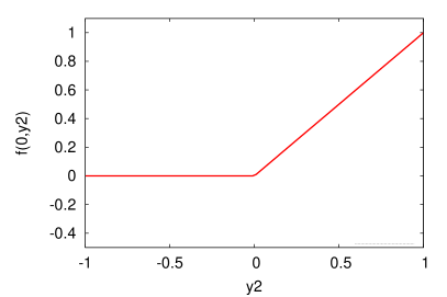
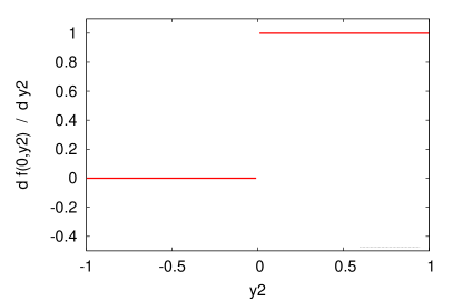
Figure 5: The left graph shows the variation of the first projection of the functor $f$ (that is, of $\max\{0,y2\}$) in the second argument (that is, of $y2$). The right graph shows the respective partial derivation in direction $y2$ on for the values on this line. In the origin (0,0) itself, $f$ is clearly not differentiable.

Let us study the effect this has on the Runge-Kutta method on an interval of size $h$, using the start value $y_{n}=(0,-\frac{1}{2}h)$. Applying RK4, we get

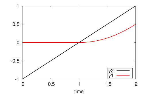
Figure 6: $y1$ and $y2$ from the solution of the ODE of the simplified example in the time interval $[0,2]$.

• $k_{1}=f\big{(}(0,-\frac{1}{2}h)\big{)}=(0,1)$,

• $k_{2}=f\big{(}(0,0)\big{)}=(0,1)$,

• $k_{3}=f\big{(}(0,0)\big{)}=(0,1)$,

• $k_{4}=f\big{(}(0,\frac{1}{2}h)\big{)}=(\frac{1}{2}h,1)$, and

• $y_{n+1}=y_{n}+\frac{1}{6}h(k_{1}+2k_{2}+2k_{3}+k_{4})=(h^{2}/12,h/2)$.

The analytical evaluation, however, provides ${\mathbf{(h^{2}/8,h/2)}}$ which differs from the provided result by $\mathbf{\frac{1}{24}h^{2}}$ in the first projection. Note that the expected difference in the first projection is in the order of $h^{2}$ if we place the point where $\max$ is in balance (the ‘swapping point’ that is related to the point where optimal strategies change) uniformly at random at some point in the interval.

Still, one could object that we had to vary both the left and the right border of the interval. But note that, if we take the initial value $y(0)=(0,-1)=y_{0}$, seek $y(2)$, and cut the interval into $2n+1$ pieces of equal length $h=\frac{2}{2n+1}$, then this is the middle interval. (This family contains interval lengths of arbitrary small size.)

0.O.2 Connection to the Bellman Equations

The first step when applying this to the Bellman equations is to convince ourselves that their functor $F=\bigotimes_{l\in L}F_{l}$ with $F_{l}=\mathit{opt}\sum\ldots$ is indeed not differentiable. We use $g$ for the arguments of $F$ in order to distinguish it from the solution $f$, where $f(t)$ is the time-bounded reachability probability at time $t$.

For this, we simply re-use the example from Figure 1. The particular functor $F$ is not differentiable in the origin: varying $F_{l_{R}}$ in the direction $g_{l}$ provides the function shown in Figure 7, showing that $F_{l_{R}}$ is not differentiable in the origin.

(Due to the direction of the evaluation, this is the ‘rightmost’ point where the optimal strategy changes.)

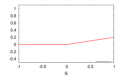
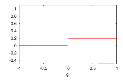
Figure 7: The left graph shows the variation of the first projection of the functor $F$ in the argument $g_{l}$ at the origin. The right graph shows the respective partial derivation in direction $g_{l}$ on for the values on this line. In the origin $\vec{0}$ itself, $F$ is clearly not differentiable.

Again, differentiating $F_{l_{R}}(f(t_{1}))$ in the direction $g_{l}$ provides a non-differentiable function. (In fact, a function similar to the function shown in Figure 7, but with adjusted $x$-axis.)

An analytical argument with $e$ functions is more involved than with the toy example from the previous subsection. However, when the mesh length (or: interval size) goes towards $0$, then the ascent of the $e$ functions is almost constant throughout the mesh/interval. In the limit, the effect is the same and the error in the order of $h^{2}$.

References

• [1] C. Baier, H. Hermanns, J.-P. Katoen, and B. Haverkort. Efficient computation of time-bounded reachability probabilities in uniform continuous-time Markov decision processes. Theoretical Computer Science, 345(1):2–26, 2005.
• [2] R. Bellman. Dynamic Programming. Princeton University Press, 1957.
• [3] M. Bozzano, A. Cimatti, M. Roveri, J.-P. Katoen, V. Y. Nguyen, and T. Noll. Verification and performance evaluation of AADL models. In ESEC/SIGSOFT FSE, pages 285–286, 2009.
• [4] T. Brázdil, V. Forejt, J. Krcál, J. Kretínský, and A. Kucera. Continuous-time stochastic games with time-bounded reachability. In Proc. of FSTTCS, pages 61–72, 2009.
• [5] P. Buchholz, E. M. Hahn, H. Hermanns, and L. Zhang. Model checking algorithms for CTMDPs. In Proc. of CAV, 2011. To appear.
• [6] P. Buchholz and I. Schulz. Numerical analysis of continuous time Markov decision processes over finite horizons. Computers and Operations Research, 38(3):651–659, 2011.
• [7] T. Chen, T. Han, J.-P. Katoen, and A. Mereacre. Computing maximum reachability probabilities in Markovian timed automata. Technical report, RWTH Aachen, 2010.
• [8] N. Coste, H. Hermanns, E. Lantreibecq, and W. Serwe. Towards performance prediction of compositional models in industrial gals designs. In Proc. of CAV, pages 204–218, 2009.
• [9] H. Garavel, R. Mateescu, F. Lang, and W. Serwe. CADP 2006: A toolbox for the construction and analysis of distributed processes. In Proc. of CAV, pages 158–163, 2007.
• [10] E. Hairer, S. P. Nørsett, and G. Wanner. Solving Ordinary Differential Equations I (2nd revised. ed.): Nonstiff Problems. Springer-Verlag, New York, 1993.
• [11] T. A. Henzinger, M. Mateescu, and V. Wolf. Sliding window abstraction for infinite Markov chains. In Proc. of CAV, pages 337–352, 2009.
• [12] A. Martin-Löfs. Optimal control of a continuous-time Markov chain with periodic transition probabilities. Operations Research, 15(5):872–881, 1967.
• [13] B. L. Miller. Finite state continuous time Markov decision processes with a finite planning horizon. SIAM Journal on Control, 6(2):266–280, 1968.
• [14] M. R. Neuhäußer, M. Stoelinga, and J.-P. Katoen. Delayed nondeterminism in continuous-time Markov decision processes. In Proc. of FOSSACS, pages 364–379, 2009.
• [15] M. R. Neuhäußer and L. Zhang. Time-bounded reachability probabilities in continuous-time Markov decision processes. In Proc. of QEST, pages 209–218, 2010.
• [16] M. Rabe and S. Schewe. Optimal time-abstract schedulers for CTMDPs and Markov games. In Proc. of QAPL, pages 144–158, 2010.
• [17] M. Rabe and S. Schewe. Finite optimal control for time-bounded reachability in continuous-time Markov games and CTMDPs. Accepted at Acta Informatica, 2011.
• [18] L. Zhang and M. R. Neuhäußer. Model checking interactive Markov chains. In Proc. of TACAS, pages 53–68, 2010.