A new limit on the Ultra-High-Energy Cosmic-Ray flux with the Westerbork Synthesis Radio Telescope

Abstract

A particle cascade (shower) in a dielectric, for example as initiated by an ultra-high energy cosmic ray, will have an excess of electrons which will emit coherent Čerenkov radiation, known as the Askaryan effect. In this work we study the case in which such a particle shower occurs in a medium just below its surface. We show, for the first time, that the radiation transmitted through the surface is independent of the depth of the shower below the surface when observed from far away, apart from trivial absorption effects. As a direct application we use the recent results of the NuMoon project, where a limit on the neutrino flux for energies above $10^{22}$ eV was set using the Westerbork Synthesis Radio Telescope by measuring pulsed radio emission from the Moon, to set a limit on the flux of ultra-high-energy cosmic rays.

I Introduction

Cosmic rays, charged particles traveling through the universe, have been observed at energies ranging from GeV to above $10^{20}$ eV Abraham:2008ru . The highest observed energies lie well above energies that can be reached by particle accelerators on Earth. These particles are of particular interest to astrophysics and particle physics to answer fundamental questions about cosmic acceleration mechanisms and particle interactions. The Astrophysics interest stems from the fact that ultra-high-energy (UHE) cosmic rays, particles with energies above $6\cdot 10^{19}$ eV have two important properties. They are less deflected by the galactic magnetic fields and therefore contain more information about their source of origin PAO-Correlation , which is still unknown. It should be noted that the real energy threshold at which this becomes apparent is dependent on the type of particle and scales with their rigidity. In addition their sources are not too far from Earth since they interact with the cosmic microwave background to produce pions and therefore experience substantial energy loss over distances of the order of 50 Mpc. This is known as the GZK-effect Greisen . To detect these particles requires a large collecting area, because the flux at 60 EeV is only $1/\rm{km}^{2}/\rm{century}$ and drops off faster than $\rm{E}^{-2.6}$. This leads to detectors like the Pierre Auger Observatory with a total collecting area of 3000 km² PAO . However, to detect particles above $10^{21}$ eV a thousand-fold increase in collecting area is expected to be needed.

As first proposed in Ref. dz89 the Moon is a suitable candidate with an area of $10^{7}\,\rm{km}^{2}$. Detection is based on the fact that when a high-energy particle interacts an avalanche reaction occurs creating a cascade (shower) of particles. The number of particles near the maximum is roughly proportional to the total energy in the avalanche and is of the order of $10^{12}$ for $10^{21}$ eV Alvarez-MunizZas98 . In this particle shower there will be a net excess of electrons due to the knock-out of atomic electrons by shower positrons and high energy photons (Compton scattering). Simulations show that this excess amounts to about 20% ZasHalzenStanev92 , consistent with experimental observations SaltzbergGorham01 . Since all particles move with almost the light velocity they are closely bunched in the longitudinal as well as the lateral direction. In a dielectric this will result in the emission of coherent Čerenkov radiation at wavelengths that are larger than the typical dimensions of the charge cloud; this is known as the Askaryan effect Askaryan . For materials like ice, salt or lunar regolith this implies coherent radiation at frequencies of 3 GHz and less ZasHalzenStanev92 and this mechanism is used in several experiments to detect high-energy cosmic neutrinos. Well known examples are the ANITA anita , GLUE glue , LUNASKA lunaska , and NuMoon Sch09 experiments.

For a particle shower deep inside the dielectric, such as is usually the case for neutrino-induced showers, the picture for the Askaryan effect clearly applies. The subject of the present work is to investigate the emitted radiation for the case that the particle shower occurs very close to the boundary between the dielectric and vacuum. In this case one can imagine that a dielectric layer of minimal thickness between the shower and vacuum is required for Čerenkov emission to occur. This relates to the concept of a formation zone/formation length for Čerenkov radiation as was introduced in Ref. Tak94 and used in calculations of the acceptance for detecting high-energy cosmic particles Gor01 .

Since neutrinos are weakly interacting particles they can traverse many hundreds of kilometers in dense materials before interacting. For neutrino-induced showers the issue of a possible formation length is thus not essential since they typically interact deep in the Moon, compared to which any formation length would be negligible. Cosmic rays are particles interacting via the strong interaction and thus induce a reaction well within a meter from the surface of a dense material. For cosmic-ray induced showers the possible existence of a formation length for the emission of electromagnetic radiation could make the difference between being able to observe the shower or not especially at wave lengths of the order of a few meters. The study we present in this paper indicates that for the motion of charged particles inside a dielectric the concept of a formation zone does not apply. We will show that due to the finiteness of a particle trajectory inside a dense medium the radiation detected in vacuum is independent of the depth of the trajectory below the surface, other than for absorption in the medium. This situation is very different from that for the opposite geometry, an effectively infinite electron beam in vacuum inducing Čerenkov emission in a dielectric, as has been investigated theoretically in Ref. Ulrich6667 and confirmed in experiments Tak00 . The essence of the difference lies in the fact that for particle showers in a medium the track length is necessarily finite for which case Čerenkov and bremsstrahlung emission cannot really be distinguished, as was already noted in Refs. Law65 ; Afa99 .

Using the new finding of an absence of a formation length for radiation emitted by a shower in a dense material we have calculated the detection probability for observing radio emission from cosmic-ray impacts on the lunar surface. The idea to observe this type of emission from the Moon with radio telescopes was first proposed by dz89 and the first experimental endeavors in this direction were carried out with the Parkes telescope parkes96 . It was shown in Ref. Sch06 that observations in the frequency range of 100-200 MHz (as suggested by Ref. FalckeGorham ) maximizes the detection probability with small loss of sensitivity. This was used in recent lunar observations with the Westerbork Synthesis Radio Telescope (WSRT) to set a new limit on the flux of ultra-high energy (UHE) neutrinos Sch09 . Combining these observational data and our present calculation of the detection efficiency we set a new limit on the flux of cosmic rays at energies in excess of $10^{22}$ eV. Such a limit is of interest since recent results of the PAO indicate a steepening in the cosmic ray spectrum at the Greisen-Zatsepin-Kuzmin (GZK) energy of $6\cdot 10^{19}$ eV PAO10 . The flux of cosmic rays above this energy will be a clear indication of nearby sources and the nature thereof. In future observations with new generation, more sensitive, synthesis telescopes this method may be used to measure the flux at GZK energies.

II Shallow Showers

The argument that a formation-zone effect will reduce the emission for shallow showers hinges on two intuitive points: one, that as the distance from the cascade to the surface decreases, the emission increasingly becomes insensitive to the presence of the dielectric; and two, that the Čerenkov radiation from such a cascade in vacuum (a gedankenexperiment) is zero. In this section, we proceed to disprove the second of these two points, and establish that current calculational methods, as used in programs to estimate the radiated intensity from particle showers in the Moon, correctly model shallow showers. As discussed at the end of this section, this is intuitively understandable, because for a finite track the actual radiation is mostly due to acceleration and deceleration of the net charge at the end-points Law65 ; Afa99 . In this process coherent radiation is emitted, known as the Askaryan effect Askaryan . As is well known Law65 ; Afa99 for finite trajectories one cannot distinguish between Čerenkov radiation and Bremsstrahlung.

We will first (in Section II.1) outline the standard approach used in the calculation of the emitted Čerenkov-radiation intensity for neutrino induced showers, and in Section II.2 describe how this has been used to calculate the acceptance for the GLUE glue , LUNASKA lunaska , NuMoon Sch09 , and other experiments. In Section II.3 we show that this double far-field approach (shower far below the surface and the observer far away from the surface) predicts that a deep cascade (excluding absorption) will produce the same observable radiation as a shower developing in the vacuum above the lunar surface. Since a near-surface cascade (i.e. a cosmic ray induced shower) is intermediary to these two extremes one thus expects the same radiation as from a deep cascade barring absorbtion effects. To show this at a more rigorous level we present in Section III an exact treatment which verifies that the current double far-field approximation gives the correct results even for shallow showers.

II.1 Čerenkov radiation from finite particle tracks

The calculation of the Čerenkov radiation arising from finite particle tracks is usually performed assuming the observer is in the far-field in an infinite dielectric medium. According to classic electromagnetic theory a shower with a current density of $J_{z}(\mathbf{r},t)=cq(z)\delta(\mathbf{r}-ct\hat{z})$ and $J_{x}=J_{y}=0$ leads in the far field (distance much greater than the shower dimension) to a vector potential

$$A_{z}(\mathbf{R},\omega)=\frac{e^{ikR}}{\sqrt{2\pi}c\,R}\int_{-\infty}^{\infty}q(z)\,e^{-iz\omega(n\cos\theta_{s}-1)/c}dz\;,$$ (1)

where $\theta_{s}$ is the angle between $\mathbf{R}$ and $\hat{z}$ as shown in Fig. (1), and $n$ is the index of refraction of the medium. The electric field can be calculated to be $E=\omega A_{z}\sin\theta_{s}$ where $\vec{E}$ lies in the plane spanned by the shower and $\mathbf{R}$, thus

$$E(\mathbf{R},\omega)= \omega\sin\theta_{s}\,\frac{e^{i\omega nR/c}}{\sqrt{2\pi}c\,R}\times$$

$$\int_{-\infty}^{\infty}q(z)\,e^{-iz\omega(n\cos\theta_{s}-1)/c}dz\;.$$ (2)

The function $E(\mathbf{R},\omega)$ can be calculated analytically for simple shower profiles Tamm39 ; ZasHalzenStanev92 ; Leh04 ; Sch06 , or can be taken from parameterisations of detailed simulation results Alvarez-MunizZas98 .

II.2 Treatment for deep cascades

Figure 1: Geometry of a particle cascade in the Moon. The ‘double-far-field’ approach assumes $R\gg d\gg L$.

Current methods to calculate the intensity of radio emission from Lunar showers use a double-far-field approximation. Using the diagram in Fig. (1), this means that the shower length $L$ is taken to be small compared to the shower depth, $a$, and the travel distance in the medium, $d$, and that the observing distance, $R$, is much larger than the shower depth. The radiation incident on the lunar surface can be taken as its far-field (i.e. in an infinite uniform medium) solution. This radiation is transmitted through the surface according to simple refraction laws and the strength at the Earth is calculated assuming the Earth-Moon distance dominates the $1/R$ term. Thus the observed radiation can be expressed as

$$E_{\rm obs}(R,\theta_{o},\omega)=t(\theta_{i},n)\,E_{\rm m}(R,\theta_{s},\omega)\,e^{-d/\ell(\omega)}\;,$$ (3)

where $t$ is the transmission coefficient, which depends on the incident angle and Lunar refractive index, and $E_{\rm m}$, given by Eq. (2), is the infinite-medium solution of the emitted radiation for the Moon’s material properties. $R$ is taken to be the Earth-Moon distance of approximately $3.884\times 10^{8}$ m, and the exponential accounts for attenuation in the medium using the frequency-dependent attenuation-length $\ell(\omega)$.

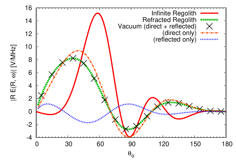
Figure 2: [color online] Radiation pattern as function of observer angle $\theta_{o}$ at 150 MHz; red drawn curve: a cascade in infinite uniform regolith; green dotted: a deep regolith cascade refracted to the vacuum; black crosses: the total observed emission from a cascade in vacuum immediately above a dielectric boundary. The ‘direct’ (orange) and ‘reflected’ (blue) components of the vacuum emission are also plotted separately. The refracted regolith and total vacuum cases are identical.

The result of Eq. (3) is plotted in Fig. (2) as a function of the observation angle $\theta_{o}$. The calculation is for the plane containing the shower axis and the surface normal, so all radiation has a parallel polarisation. Also, we take the case of a cascade parallel to the surface ($\alpha=0$), so Snell’s law becomes $n\cos\theta_{s}=\cos\theta_{o}$. We use Eq. (2) to calculate $E_{\rm m}$ for a constant charge excess $q=-10^{12}~{}e$ moving over a distance $L=3.0$ m at velocity $v=c$. The observation frequency is taken as $\nu=150$ MHz, and the regolith refractive index as $n=1.8$. For waves diverging from a point-source, the transmission coefficient for parallel polarisation is

$$t_{||}(\theta_{s},n)=\frac{2\sin\theta_{o}}{n\sin\theta_{o}+\sin\theta_{s}}\;$$ (4)

since for $\alpha=0$ we have $\sin{\theta_{s}}=\cos{\theta_{i}}$.

II.3 Emission in a vacuum

The double-far-field treatment of Section II.2 may be expected to break down as the distance $d$ of the cascade to the surface becomes small. To place a simple limit on near-surface effects, consider the following extreme case: a cascade developing immediately above the surface. In this case, the radiation seen by an observer will be that produced in vacuum ($n=1$), but consist of both direct and reflected components, with zero path difference due to the proximity of the interface. For $\alpha=0$ the radiated electric field is thus

$$E_{\rm obs}(R,\theta_{o},\omega)=\left(1+r(\theta_{o},n)\right)E_{\rm v}(\theta_{o},\omega)$$ (5)

where $E_{\rm v}$ is the radiation expected from a cascade in an infinite vacuum, and $r$ is the Fresnel reflection coefficient (identical for plane and spherical waves). Using Eq. (2) for $E_{\rm v}$, radiation of some magnitude will be emitted. In Fig. (2) the result from Eq. (5) is shown using the same parameters as used in the double-far-field approximation in Section II.2. For the sake of clarity we also plot the direct and reflected contributions from Eq. (5) separately, which add to give exactly the same radiation pattern as that from Eq. (3) for $d=0$. That is, the emission seen by an observer from a cascade immediately above a dielectric boundary is exactly the same as that from a cascade immediately below the surface, which in turn is identical to that from a deep cascade if absorption in the medium is been ignored. It can be shown analytically in the case $\alpha=0$ that the two equations give identical results for an arbitrary mix of perpendicular and parallel polarisations.

It seems counter-intuitive that any Čerenkov radiation is viewed from a cascade parallel to the surface, since radiation emitted at the Čerenkov angle will be totally internally reflected. The solution to this apparent contradiction lies in the fact that for a shower of finite length the emitted radiation has a large spread around the Čerenkov angle (see for example Ref. Law65 ; Sch06 ). For a shower in a medium only the radiation emitted at angles larger than the Čerenkov angle will penetrate the surface while for a theoretical shower in vacuum the Čerenkov angle lies at zero degrees. Alternatively one may regard a shower of finite extent as corresponding to the acceleration and deceleration of charge at the beginning and end of the shower Law65 ; Afa99 (equal to the appearance and disappearance of a moving charge), a picture which has also been used to explain the emission of electromagnetic radiation of showers induced in air MGMR .

These results indicate that there will be no change in the observed radiation as the particle distribution induced by a UHE particle interaction lies close to the surface. In the following section this is shown using a more rigorous method.

III Exact calculation for near-surface showers

For shallow showers, such as those from UHE cosmic-ray interactions with the lunar surface, no far field approximation can be made for the radiation reaching the surface. For the calculation in the previous section this was an essential assumption. We avoid making this approximation by performing a complete wave-equation calculation.

In the following derivation we consider two half-spaces divided by the plane $x=0$. For $x>0$ the refraction index is $n^{\prime}$ (=1 for vacuum). For $x<0$ the refraction index is $n$ (=1.8 for the moon). In the lower half plane a particle with charge $Q$ and velocity $\beta$ moves from $z=-L/2$ to $z=L/2$ at $x=-a$, $y=0$, passing through $z=0$ at $t=0$ which corresponds to the same geometry as studied in the previous section. The four-vector potential for this system is determined by the Maxwell equations. Care should be taken since the index of refraction is different for the two sides of the boundary.

In the present discussion it is sometimes easier to work in the space-time domain, sometimes with energy and momentum. The relation between the two is given by the usual Fourier transformation

$$\mathbf{A(r},t)=\int\!\frac{d^{3}k\,d\omega}{4\pi^{2}}\mathbf{A(k},\omega)\,e^{i\mathbf{k\cdot r}-i\omega t}\;.$$ (6)

In a homogeneous medium with refraction index $n$ the vector potential can be calculated Jackson from

$$[k^{2}-\frac{n^{2}\omega^{2}}{c^{2}}]\,\Phi(\mathbf{k},\omega) =\frac{4\pi}{n^{2}}\rho(\mathbf{k},\omega)$$

$$[k^{2}-\frac{n^{2}\omega^{2}}{c^{2}}]\,\mathbf{A}(\mathbf{k},\omega) =\frac{4\pi}{c}\mathbf{J}(\mathbf{k},\omega)\;.$$ (7)

For the problem under consideration the charge density is

$$\rho(\mathbf{r},t)=q(z)\,\delta(\mathbf{r}-\mathbf{v}t-\mathbf{a})\;,$$ (8)

and the current density is

$$\mathbf{J}(\mathbf{r},t)=\mathbf{v}\,\rho(\mathbf{r},t)\;,$$ (9)

with $\mathbf{v}$ the velocity of the charge, $\mathbf{a}=-a\hat{x}$ the distance under the surface, and $q(z)$ the charge of the particle. The vector potential can now be written as

$$\mathbf{A(k},\omega)=4\pi\frac{\mathbf{v}}{c}\frac{\rho(\mathbf{k},\omega)}{k^{2}-\frac{n^{2}\omega^{2}}{c^{2}}}\;,$$ (10)

with

$$\rho(\mathbf{k},\omega)=\frac{Q}{\beta c}\frac{e^{ik_{x}a}\sin{(\frac{L}{2}(k_{z}-\frac{\omega}{\beta c})})}{2\pi^{2}(k_{z}-\frac{\omega}{\beta c})}\;.$$ (11)

Note that because $\mathbf{v}$ is only non-zero in the $z$-direction, $A_{z}$ is the only non-vanishing component of $\mathbf{A}$.

The transmission coefficient for the vector potential can be derived from the field equations across the boundary. In general this is not easy, however, for the special case of interest here, this can be done by considering the electric field in the $y=0$ plane. For electric fields generated by a vector potential of the form $A_{i}(r,t)=A_{i}^{0}e^{i(k_{x}x+k_{y}y+k_{z}z-\omega t)}$ we obtain $E_{i}=\partial_{0}A_{i}-\partial_{i}A_{0}$, and thus $E_{||}=E_{x}\hat{x}\cdot\hat{||}+E_{z}\hat{z}\cdot\hat{||}=i\frac{\omega}{c}\frac{k_{z}}{k}A_{x}^{0}-i\frac{\omega}{c}\frac{k_{x}}{k}A_{z}^{0}$. For the field of the transmitted wave we may write $E_{||}^{\prime}=t_{||}E_{||}$. In our treatment it is sufficient to calculate $A_{z}^{\prime}$ since only $A_{z}$ is non-vanishing,

$$t_{A_{z}||}=\frac{{A_{z}^{0}}^{\prime}}{A_{z}^{0}}=\frac{k_{x}}{kE_{||}}\frac{E^{\prime}_{||}k^{\prime}}{k_{x}^{\prime}}=t_{E||}\frac{k_{x}}{k}\frac{k^{\prime}}{k_{x}^{\prime}}\;,$$ (12)

where $t_{E||}=2\cos\theta_{i}/(n^{\prime}/n\cos\theta_{i}+\cos\theta_{t})$ (see Fig. (1) for the definition of the angles) is the transmission coefficient of the electric field. At this point we have made the implicit assumption that the observer is far from the surface and that the outgoing waves can be treated as plane waves. We still perform a complete integral over all waves leading from the source to the surface. For transmission parallel to the surface we thus derive that

$$t_{A_{z}||}=\frac{2k_{x}^{2}}{k_{x}k_{x}^{\prime}+\frac{n^{2}}{n^{\prime 2}}k_{x}^{\prime 2}}\;,$$ (13)

where $k_{x}^{2}=\frac{n^{2}\omega^{2}}{c^{2}}-k_{y}^{2}-k_{z}^{2}$ and $k_{x}^{\prime}=k_{x}\sqrt{1-\frac{(n^{2}-n^{\prime 2})\omega^{2}}{c^{2}k_{x}^{2}}}$.

An incoming wave $e^{i\mathbf{k\cdot r}-i\omega t}$ generates for $x>0$ a transmitted wave $t_{A_{z}||}e^{i\mathbf{k^{\prime}\cdot r}-i\omega t}$ where $t_{A_{z}||}$ is given by Eq. (13). The transmitted radiation ($x>0$) can now be expressed as

$${A}_{z}^{\prime}(\mathbf{r},t)=\int\!\frac{d^{3}k\,d\omega}{4\pi^{2}}\frac{2k_{x}^{2}}{k_{x}k_{x}^{\prime}+\frac{n^{2}}{n^{\prime 2}}k_{x}^{\prime 2}}A_{z}(\mathbf{k},\omega)e^{i\mathbf{k^{\prime}\cdot r}-i\omega t}\;,$$ (14)

where ${A}_{z}(\mathbf{k},\omega)$ is given by Eq. (10) and $\mathbf{k^{\prime}}$ is a function of $\mathbf{k}$.

To evaluate this expression, first a change of variables is made to wave vectors in the $n^{\prime}$ medium, $k_{x}^{\prime}=\sqrt{k_{x}^{2}-\frac{n^{2}-n^{\prime 2}}{c^{2}}\omega^{2}}$, $k_{y}^{\prime}=k_{y}$, $k_{z}^{\prime}=k_{z}$. Subsequently $\omega$ is integrated over by extending the integral into the complex plane where the contributions of the poles of $\frac{1}{k^{\prime 2}-\frac{n^{\prime 2}\omega^{2}}{c^{2}}}$ in $A_{z}(\mathbf{k},\omega)$ have to be considered. The poles are calculated by adding an infinitesimal imaginary part to account for causal propagation. This leads to the limitation $\beta ct>L/2$. As the next step the $d^{3}k^{\prime}$ integral is written as $dk^{\prime}\sin{\theta}\,d\theta\,d\phi$ where $k_{x}^{\prime}=k^{\prime}\cos\theta$, $k_{y}^{\prime}=k^{\prime}\sin\theta\sin\phi$ and $k_{z}^{\prime}=k^{\prime}\sin\theta\cos\phi$. The integrals can now be reduced to two integrals of the form $\int_{-\infty}^{\infty}dk^{\prime}\,e^{ik^{\prime}f(\theta,\phi)}$. After integrating over $k^{\prime}$ this gives a delta function which can be used to perform the integral over $\phi$. The field can now be expressed as

$$A_{z}(\mathbf{r},t)=A_{z}^{(1)}(\mathbf{r},t)+A_{z}^{(2)}(\mathbf{r},t)$$ (15)

where the first contribution is

$$A_{z}^{(1)}(\mathbf{r},t)=\frac{-Q}{\pi n^{\prime}}\int\sin{\theta}\,d\theta\frac{W(\theta)\,(z+\frac{L}{2})+\frac{\eta^{2}}{n^{\prime}\beta}}{W^{2}(\theta)+\frac{2W(\theta)\,(z+\frac{L}{2})}{n^{\prime}\beta}+\frac{\eta^{2}}{n^{\prime 2}\beta^{2}}-y^{2}\sin^{2}\theta}T_{4}\,Re\left[\frac{1}{\sqrt{\eta^{2}\sin^{2}\theta-W^{2}(\theta)}}\right]\;,$$ (16)

and the second contribution is

$$A_{z}^{(2)}(\mathbf{r},t)=\frac{Q}{\pi n^{\prime}}\int\sin{\theta}\,d\theta\frac{\tilde{W}(\theta)\,(z-\frac{L}{2})+\frac{\tilde{\eta}^{2}}{n^{\prime}\beta}}{\tilde{W}^{2}(\theta)+\frac{2\tilde{W}(\theta)\,(z-\frac{L}{2})}{n^{\prime}\beta}+\frac{\tilde{\eta}^{2}}{n^{\prime 2}\beta^{2}}-y^{2}\sin^{2}\theta}T_{4}\,Re\left[\frac{1}{\sqrt{\tilde{\eta}^{2}\sin^{2}\theta-\tilde{W}^{2}(\theta)}}\right]\;,$$ (17)

where

$$W(\theta) =x\cos\theta+a\cos\theta\sqrt{1+\frac{n^{2}-n^{\prime 2}}{n^{\prime 2}\cos^{2}\theta}}-ct/n^{\prime}-\frac{L}{2n^{\prime}\beta}\;,$$

$$\tilde{W}(\theta) =x\cos\theta+a\cos\theta\sqrt{1+\frac{n^{2}-n^{\prime 2}}{n^{\prime 2}\cos^{2}\theta}}-ct/n^{\prime}+\frac{L}{2n^{\prime}\beta}\;,$$

$$T_{4} =\frac{2\cos\theta}{\cos\theta\sqrt{1+\frac{n^{2}-n^{\prime 2}}{np^{2}\cos^{2}\theta}}+\frac{n^{2}}{n^{\prime 2}}\cos\theta}\;,$$

$$\eta^{2} =(z+\frac{L}{2})^{2}+y^{2}\;,$$

$$\tilde{\eta}^{2} =(z-\frac{L}{2})^{2}+y^{2}\;,$$ (18)

Note that only the real part of the square root contributes because of the restriction $W(\theta)\leq\eta\sin{\theta}$ which is imposed by the $\delta$-function in the derivation.

III.1 Checking limiting cases

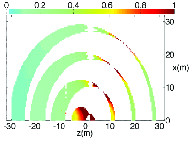
Figure 3: [color online] The vector potential $A_{z}$ for $y=0$ in the near field at different times $ct$=5, 9, 13, 17 m; $n=n^{\prime}$=1.8, $a$=0, and $L$=4 as a function of $x$ and $z$. The absence of field near $z=2$ is due to numerical difficulties.

In Fig. (3) the vector potential is plotted in the $y=0$ plane for different times shortly after creation for a homogeneous medium. It shows an outgoing pulse traveling at the light velocity which is stronger and of shorter duration in the direction of the Čerenkov cone. At angles away from the Čerenkov angle the waves emitted from different parts for the current distribution no longer arrive at the same time. This is reflected in Fig. (3) by a broadening of the pulse which has the immediate consequence that the signal is coherent only for lower frequencies.

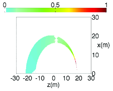
Figure 4: [color online] $A_{z}$ for $n$=1.8, $n^{\prime}$=1.0 at $ct$=20 m, $L$=4, and $a$=1. The absence of field near $z=2$ is due to numerical difficulties.

When we include refraction into vacuum the outgoing wave has a different structure as shown in Fig. (4). Because of the refraction at the surface the Čerenkov angle is projected at zero degrees, however, there is still radiation transmitted through the surface.

The electric field can be calculated from the vector potential using $E(\mathbf{R},\omega)=\omega\sin{\theta}(A_{z}^{(1)}(\mathbf{R},\omega)+A_{z}^{(2)}(\mathbf{R},\omega))$. The Fourier transform is calculated numerically by taking the sum $A_{3}^{(i)}(\mathbf{R},\omega)=\sum_{t=t_{0}}^{t_{1}}e^{i\omega t}A_{3}^{(i)}(\mathbf{R},t)\Delta t/\sqrt{2\pi}$ where $A_{3}^{(i)}(\mathbf{R},t)$ is calculated numerically at each point. For a shower far below the surface ($a>>L$) viewed from far away ($R>>a$) this should give the same result as the analytic result Eq. (3). In Fig. (5) both the double far field analytic result and the exact numerical result are compared for two different observing frequencies, showing that both results are practically indistinguishable.

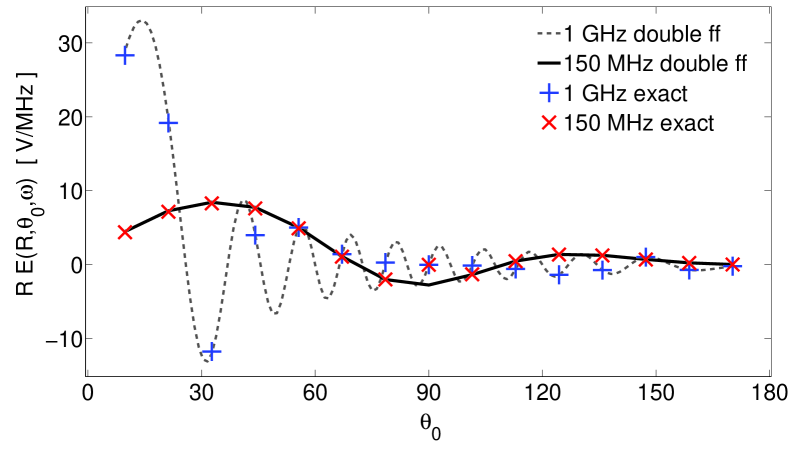
Figure 5: [color online] Electric field strength as a function of angle at 150 MHz and 1 GHz at a distance of 1400 km for a shower length of 3 m, and a charge of $Q=10^{12}$e, calculated according to the double far-field analytic (see Section II.1) and the exact numerical (see Section III) methods.

III.2 Formation zone effects

After having checked the calculation in the far-field regime we can use it to calculate the shower at distances close to the surface. The result of the calculation is shown in Fig. (6) for 3 different angles. This shows that within an accuracy of 1.5% the field is the same for showers at depths ranging from 1 cm to 1 km when observed from sufficiently far away. The error we attribute to the numerical calculation and as a second order effect in $a/R$ and is largest for the calculation for $a=1$ km. The important implication of this is that for an observer at Earth the observed electric field is independent of depth below the lunar surface. There is no shallow shower effect which supports the conclusion arrived at in Section II.3.

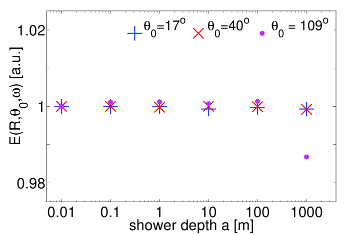
Figure 6: [color online] Electric field strength as a function of depth, normalized to that at $a=10^{-2}$ m, for 3 different angles at 150 MHz at a distance of 1400 km for a shower length of 3 m.

IV New limit on the UHECR flux

As a first application we will use the present result to obtain limits on the flux of UHE cosmic rays using the results presented in a recent publication of the ‘NuMoon’ observations of the Moon using the Westerbork Synthesis Radio Telescope (WSRT) Sch09 . The WSRT consists of an array of 14 parabolic antennas of 25 m diameter on a 2.7 km East-West line. In the observations we used the Low Frequency Front Ends (LFFEs) which cover the frequency range 115–180 MHz with full polarization sensitivity. The Pulsar Machine II (PuMa II) backend kss08 can record a maximum bandwidth of 160 MHz, sampled as 8 subbands of 20 MHz each. Only 11 of the 12 WSRT dishes with equal spacing were used for this experiment. In these observations as part of the NuMoon project, the radio spectrum was searched for short, nano-second pulses emitted from showers induced in the lunar regolith by UHE neutrinos. The data allowed a tightening of the bounds on the neutrino flux at high energies Sch09 .

When an UHE neutrino interacts, most of the energy is carried away by the emerging lepton which, in general, does not produce a detectable signal while only about 20% of the energy is deposited in a hadronic shower which emits a signal that can be detected at Earth. When a cosmic ray impinges on the lunar surface all its energy will be converted into a hadronic cascade of energetic particles. This cascade will commence right at the surface and the shower maximum is thus within meters from the surface. Due to the absence of a formation zone these events should thus also give a signal of the characteristics of the ones that were searched for in the observations of Ref. Sch09 . With its surface area of the order of $10^{7}$ km², our finding of the absence of a formation zone thus shows that the Moon can be used as a sensitive cosmic-ray detector.

As the first step in the WSRT observations the narrow band Radio Frequency Interference (RFI) is filtered from the recorded time series data for each subband (with a sampling frequency of 40 MHz) and the dispersion due to the ionosphere of the Earth is corrected for. Short, nano-second, pulses emitted from the Moon correspond to strong pulses with large bandwidth. To search for these pulses 5-time-sample-summed power spectra (so called $P_{5}$-spectra) were constructed for all subbands. The data were kept for further processing when in all four subbands beamed at the same side of the Moon a value for $P_{5}$ larger than a certain threshold was found within a certain maximum time offset. In a subsequent analysis additional constraints were imposed, such as eliminating pulses that had a long time duration and pulses that were found in both beams within a certain time limit. The largest remaining pulse had a strength of $S=152$ kJy which is a factor 3 larger than expected for pure statistical noise. To account for dead-time issues and filtering inefficiencies a complete simulation of the data taking was performed where short pulses with a random time offset have been added to the raw data (considered as background). The detection efficiency (DE) was determined as the fraction of inserted pulses that is retrieved after applying all trigger conditions and cuts that were used in the analysis. The System Equivalent Flux Density (SEFD) for the WSRT, averaged over the frequency range under consideration, is $\sigma^{2}=400$ Jy per time sample.

A more detailed description of the followed procedure can be found in Ref. Sch09 where it is concluded that in 46.7 hours of observation no pulses from the Moon were detected with a strength exceeding $240$ kJy with a 87.5% probability. Simulation calculations have been performed to convert this to a flux limit. In the simulation cosmic rays of a certain energy $E_{s}$ hit the lunar surface at arbitrary angles and create a particle cascades. Based on Monte Carlo simulations the intensity of radio-waves emitted from such a cascade in the lunar regolith have been parameterized as function of emission angle and frequency Zas92 ; Alv01 ; Gor04 . The emitted radiation is passed through the lunar surface following the usual laws of wave refraction which, due to the absence of formation zone effects, also applies to the case where the particle cascade occurs just below the surface. From the surface of the Moon to Earth the intensity follows the usual inverse square law. The details of the simulations are described in detail in Ref. Sch06 . Using the model-independent procedure described in Ref. Leh04 the non-observation of pulses of a certain strength can thus be converted in an energy-dependent 90% confidence limit on the cosmic-ray flux as shown in Fig. (7) by running the simulation for different values of $E_{s}$. In the simulations the effects of surface roughness can be ignored Sch06 .

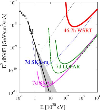
Figure 7: [color online] The currently established cosmic-ray flux limit from WSRT observations Sch09 (thick red drawn line) is compared to the flux determined by the Pierre Auger Observatory Abraham:2010mj (data points with error bars) and a simple polynomial expansion (black line, see text). Also the prospective flux sensitivities are indicated that can be obtained with LOFAR LOFAR and SKA SKA observations.

The present limit for the flux of cosmic rays that follows from the existing WSRT observations Sch09 is well above what could be expected based on the observations made by the Pierre Auger Observatory Abraham:2010mj . The thin dotted straight line in Fig. (7) shows the model-independent differential flux limit, comparable to the presently set limits, for observations of the Pierre Auger Observatory, showing that the limit set by the WSRT observations is considerably lower albeit at considerably higher energies. The thick line corresponds to a polynomial expansion $~{}E^{-4.3}$ as advocated in Ref. Abraham:2010mj where the grey band corresponds to an uncertainty in the exponent of 0.8. The lower limit of the exponent has been taken from Ref. HiRes . The quoted values for the flux in Ref. HiRes lie well above the ones shown in Fig. (7) which might be due to an uncertainty in the energy calibration Abraham:2010mj . Future observations with new-generation radio telescopes such as LOFAR LOFAR or SKA SKA should reach much higher sensitivity for pulse detection, resulting in correspondingly lower energy thresholds as shown in Fig. (7). We show the sensitivity that can be reached in a one week measurement using the LOFAR telescope where the drawn curve uses only the core stations (SEFD of 93 Jy, using 50 MHz bandwidth) while the long-dashed curve uses all E-LOFAR stations (SEFD of 30 Jy, using full bandwidth). We have assumed here a 100% moon coverage and a detection threshold of $6\sigma$ where $\sigma$ is the amplitude of the noise. In a one week measurement with the future SKA telescope (SEFD of 1.8 Jy) the results depend on the frequencies used for the observation. At lower frequencies (100-300 MHz band, SKA-l in Fig. (7)) one is sensitive to a smaller flux while at intermediate frequencies (300-500 MHz band, SKA-m in Fig. (7)) one is sensitive to cosmic-rays of lower energy. The increased sensitivity will make this method sensitive to cosmic ray energies of the order of $10^{20}$ eV where, due to the large collecting area, competitive measurements are possible.

V Conclusions

We have shown that the concept of a formation zone does not apply for the emission of electromagnetic radiation from a moving charge distribution over a finite distance inside a dielectric emitting Čerenkov radiation. In particular we have considered the system where the charges move at close proximity to the surface separating the dielectric and vacuum. We have shown that the radiation penetrating the surface is independent of the distance of the charge distribution to the surface even for distances that are much smaller than the wavelength, provided the observer is sufficiently far away from the surface. In principle we have shown the absence of a formation zone only for a charge distribution with a block profile, however, the superposition principle can be used to show that this conclusion extents to showers with a realistic profile.

One field where this finding has a large impact is in the calculation of the acceptance of large scale cosmic-ray and neutrino detectors. As one application we have calculated the acceptance of the observations for the NuMoon project to cosmic rays and used this to derive a limit on the flux of cosmic rays for energies in excess of $2\times 10^{22}$ eV. If there would have been a formation length of the order of the wavelength of the observed radiation, the acceptance would be vanishingly small. We instead find that this approach will offer a competitive means of detecting the flux of cosmic rays with energies in excess of $10^{20}$ eV with future synthesis radio telescopes.

- (1) J. Abraham et al. [Pierre Auger Collaboration], Phys. Rev. Lett. 101, 061101 (2008).
- (2) J. Abraham et al. [Pierre Auger Collaboration], Astropart. Phys. 29, 188 (2008).
- (3) K. Greisen, PRL 16 (1966) 748; G.T. Zatsepin, V.A. Kuzmin, JETP Lett. 4 (1966) 78.
- (4) J. Abraham et al. [Pierre Auger Collaboration], arXiv:0906.2189v2 [astro-ph.HE].
- (5) R.D. Dagkesamanskii, I.M. Zheleznykh, Sov. Phys. JETP Lett. 50, 233 (1989).
- (6) J. Álvarez-Muñiz, E. Zas, Phys. Lett. B 434, 396 (1998).
- (7) E. Zas, F. Halzen, T. Stanev, Phys. Rev. D 45, 362 (1992).
- (8) D. Saltzberg et al., Phys. Rev. Lett. 86, 2802 (2001).
- (9) G.A. Askar’yan, Sov.Phys.JETP, 14 (1962) 441; 48 (1965) 988.
- (10) P.W. Gorham et al., Phys. Rev. Lett. 103, 051103 (2009).
- (11) P.W. Gorham et al., Phys. Rev. Lett. 93, 41101 (2004).
- (12) C.W. James et al., Phys. Rev. D 81, 042003 (2010).
- (13) O. Scholten et al., Phys. Rev. Lett. 103, 191301 (2009); S. Buitink et al., Astron. & Astroph. 510, A47 (2010); arXiv:1004.0274v1 [astro-ph.HE].
- (14) T. Takahashi, et al, 1994, Phys. Rev. E 50, 4041 (1994).
- (15) also fig 6 in P.W. Gorham et al, J. Phys. Soc. Jap. 70, 38 (2001); P.W. Gorham, K.M. Liewer, and C.J. Naudet, arXiv:astro-ph/9906504v1.
- (16) R. Ulrich, Z. Phys. 194, 180 (1966); Z. Phys. 199, 171 (1967).
- (17) T. Takahashi, et al., Phys. Rev. E 62, 8606 (2000).
- (18) J.D. Lawson, Am. J. Phys.33, 1002 (1965).
- (19) G.N. Afanasiev, V.G. Kartavenko, and Yu.P. Stepanovsky, J. Phys. D: Appl. Phys. 32, 2029 (1999).
- (20) T.H. Hankins, R.D. Ekers, J.D. O’Sullivan, MNRAS 283, 1027 (1996).
- (21) O. Scholten et al., Astropart. Phys. 26, 219 (2006).
- (22) H. Falcke,P.W. Gorham, Astropart. Phys. 19, 477 (2003)
- (23) Pierre Auger Collaboration (Abraham et al.), Phys.Lett. B 685, 239 (2010).
- (24) N.G. Lehtinen et al., Phys. Rev. D 69, 013008 (2004).
- (25) I.E. Tamm, J. Phys. Moscow 1, 439 (1939).
- (26) O. Scholten, K. Werner and F. Rusydi, Astropart. Phys. 29, 94 (2008); K. Werner and O. Scholten, Astropart. Phys. 29, 393 (2008); O. Scholten and K. Werner, Nucl. Instrum. Meth. A 604, S24 (2009).
- (27) J.D. Jackson, Classical Electrodynamics, edition, John Wiley & Sons, New Jersey (1998).
- (28) R. Karuppusamy, B. Stappers, and W. Van Straten, Publ. Astron. Soc. Pacific, 120, 191 (2008), astro-ph/0802.2245v1.
- (29) E. Zas, F. Halzen, and T. Stanev, Phys. Rev. D 45, 362 (1992); J. Alvarez-Muñiz and E. Zas, Phys. Lett. B 411, 218 (1997).
- (30) J. Alvarez-Muñiz, R. A. Va zquez, and E. Zas, Phys. Rev. D 61, 23001 (99); J. Alvarez-Muñiz and E. Zas, astr-ph/0102173, in “Radio Detection of High Energy Particles RADHEP 2000”, AIP Conf. Proc. No. 579 (AIP, New York, 2001).
- (31) P. Gorham et al., Phys. Rev. Lett. 93, 41101 (2004).
- (32) J. Abraham et al. [The Pierre Auger Collaboration], “Measurement Of The Energy Spectrum Of Cosmic Rays Above Ev Using The Pierre Auger Observatory,” Phys. Lett. B 685, 239 (2010)
- (33) R. U. Abbasi et al. [HiRes Collaboration], Astropart. Phys. 32, 53 (2009).
- (34) http://www.lofar.org/.
- (35) http://www.skatelescope.org/.