The Redshift Distribution of Giant Arcs in the Sloan Giant Arcs Survey

Abstract

We measure the redshift distribution of a sample of $28$ giant arcs discovered as a part of the Sloan Giant Arcs Survey (SGAS). Gemini/GMOS-North spectroscopy provides precise redshifts for $24$ arcs, and “redshift desert” constraints for the remaining $4$. This is a direct measurement of the redshift distribution of a uniformly selected sample of bright giant arcs, which is an observable that can be used to inform efforts to predict giant arc statistics. Our primary giant arc sample has a median redshift $z=1.821$ and nearly two thirds of the arcs – $64\%$ – are sources at $z\gtrsim 1.4$, indicating that the population of background sources that are strongly lensed into bright giant arcs resides primarily at high redshift. We also analyze the distribution of redshifts for $19$ secondary strongly lensed background sources that are not visually apparent in SDSS imaging, but were identified in deeper follow-up imaging of the lensing cluster fields. Our redshift sample for the secondary sources is not spectroscopically complete, but combining it with our primary giant arc sample suggests that a large fraction of $all$ background galaxies which are strongly lensed by foreground clusters reside at $z\gtrsim 1.4$. Kolmogorov-Smirnov (KS) tests indicate that our well-selected, spectroscopically complete primary giant arc redshift sample can be reproduced with a model distribution that is constructed from a combination of results from studies of strong lensing clusters in numerical simulations, and observational constraints on the galaxy luminosity function.

1. Introduction

Comparisons of the observed giant arc counts against theoretical predictions provide a test for cosmological models of structure formation. Giant arc statistics depend on the growth of structure through the abundance and internal properties of the most massive galaxy clusters that dominate the giant arc cross-section. Bartelmann et al. (1998) suggested that there was an apparent order-of-magnitude discrepancy between the observed counts of giant arcs on the sky, and what is predicted by a $\Lambda$CDM cosmology. Subsequent comparisons of homogeneous samples of giant arcs against theoretical predictions have provided additional evidence for an apparent “giant arc problem” (Gladders et al., 2003; Zaritsky & Gonzalez, 2003). Gladders et al. (2003) present a sample of five giant arcs that are identified in the Red-Sequence Cluster Survey (RCS), and Zaritsky & Gonzalez (2003) identified three strongly lensed systems in the Las Campanas Distant Cluster Survey (LCDCS), but both of these samples are very small and are therefore subject to prohibitively large uncertainties due to small number statistics.

Further studies have explored a variety of potential factors that could help to explain the underabundance of giant arcs predicted by theoretical models, such as accounting for galaxies by painting them onto simulated dark matter halos (Flores et al., 2000; Meneghetti et al., 2000; Puchwein & Hilbert, 2009), steepening of the gravitational potential in cluster cores due to baryonic dissipation effects (e.g., Puchwein et al., 2005; Rozo et al., 2008), contributions from secondary structures along the line of sight (Puchwein & Hilbert, 2009), accounting for short time-scale increases in the lensing cross-sections of halos due to mergers (Torri et al., 2004), and varying the redshift distribution of the population of background sources available to be strongly lensed into giant arcs (Hamana & Futamase, 1997; Oguri et al., 2003; Wambsganss et al., 2004). Hennawi et al. (2007) found this last factor – the background source distribution – to be the one of the leading sources of uncertainty in their efforts to produce precise estimates for giant arc statistics from ray-tracing of dark matter simulated halos for a given cosmology. The primary motivation for studying giant arc statistics in a cosmological context is to provide a comprehensive test for models of large scale structure, which require $a$ $priori$ constraints other model inputs, such as the properties of the background source population. Fortunately, the redshift distribution of giant arcs is directly observable given a sufficiently large and well-selected sample of giant arcs with redshift measurements. Samples of giant arc redshifts exist in the literature, including the catalog compiled by Sand et al. (2005) and the redshifts used by Richard et al. (2009), but they cannot be used to study the true redshift distribution of arcs because of their non-uniform selection and severe spectroscopic incompleteness.

In this letter we measure the redshift distribution of a spectroscopically complete sample of $28$ giant arcs that were discovered in the Sloan Giant Arc Survey (SGAS; M. D. Gladders et al., in preparation) and targeted for multi-object spectroscopy with Gemini/GMOS-North. We also consider a secondary sample of redshifts that were measured for an additional $19$ strongly lensed sources. For comparison we test the redshift distributions of our primary and secondary samples against simple models for the redshift distribution of giant arcs.

All magnitudes given in this letter are AB, calibrated relative to the SDSS (York et al., 2000).

2. Data and Samples

2.1. Giant Arc Redshift Sample

The lensed background sources discussed in this letter are located near the cores of foreground massive galaxy clusters with a median redshift, $z_{l}=0.435$, and a median dynamical mass, $M_{Vir}=7.84\times 10^{14}M_{\sun}h_{0.7}^{-1}$ (Bayliss et al., 2011).

We take published spectroscopic redshifts from Bayliss et al. (2011), and use optical colors combined with the absence of specific spectral features to identify upper and lower redshift bounds for some arcs that lack precise spectroscopic redshifts. Given the spectral coverage of the Gemini/GMOS spectroscopy presented in Bayliss et al. (2011) we expect to observe one or more prominent emission lines (e.g. O[II] $\lambda 3727$Å, H-$\beta~{}\lambda 4861$Å, O[III] $\lambda 4959,5007$Å  and H-$\alpha~{}\lambda 6563$Å) for galaxies at $z\lesssim 1.5$ that are actively star-forming, with some slight variation in this redshift limit that depends on the exact spectral coverage for each source. For strongly lensed sources at $1.5\lesssim z\lesssim 3.3$ we must rely on rest-frame UV features to measure redshifts, but the strength of these features can vary significantly depending on the physical properties of the individual galaxies. At redshifts of $z\gtrsim 3.3$ we expect to see a broadband flux decrement that would be indicative of the Lyman-$\alpha$ Forest and Lyman Limit being redshifted well into the $g-$band, as well as strong absorption or emission from Lyman-$\alpha~{}\lambda 1216$Å  redshifted into our data for sources with spectral coverage extending sufficiently blueward.

Using the criteria outlined above we identifty six arcs in the Bayliss et al. (2011) Gemini/GMOS data for which we can confidently place lower and upper limits on the redshifts. These six arcs all have blue colors in the available photometry, indicating that they are actively star-forming, and their optical spectra consist of blue continuum emission with no strong absorption or emission features. The precise redshift constraints vary slightly from arc to arc, depending on the exact limits of the wavelength coverage, and are given in Table 1.

Table 1Redshift Constraints from Gemini Spectroscopy

Cluster Core	Label	$z_{arc}$ range	$l/w$	Rarc	AB Mag	Source Type
SDSS J1028+1324	C	$1.58\leq z\leq 3.3$	$14$	$17\arcsec$	$g=22.81$	Primary
SDSS J1115+5319	A	$1.45\leq z\leq 3.2$	$10$	$31\arcsec$	$g=23.03$	Secondary
SDSS J1152+0930	D	$1.56\leq z\leq 3.3$	$18$	$14\arcsec$	$g=22.54$	Primary
GHO 132029+315500	A	$1.5\leq z\leq 3.3$	$20$	$21\arcsec$	$g=22.59$	Secondary
SDSS J1446+3033	F	$1.45\leq z\leq 3.3$	$7$	$15\arcsec$	$g=22.42$	Primary
SDSS J1456+5702	B	$1.55\leq z\leq 3.3$	$7$	$17\arcsec$	$g=20.83$	Primary

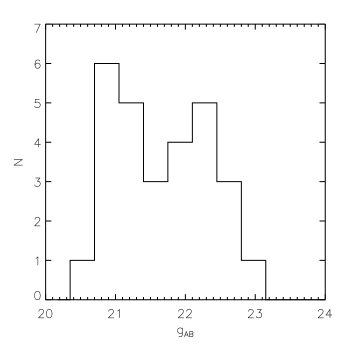
Figure 1.— Histogram of $g-$band magnitudes for the $28$ primary giant arcs discussed in this letter.

2.2. Primary Giant Arc Sample

Arcs in our primary giant arc sample meet two criteria: 1) they were visually identified in the original SDSS imaging data $and$ 2) they were were observed spectroscopically with Gemini/GMOS-North. Our primary giant arcs span a range in integrated $g-$band magnitude of $20.69\leq g\leq 22.81$ (Figure 1). This sample includes all sources identified as primary giant arcs in Bayliss et al. (2011), plus four additional arcs with redshift desert constraints as described in Section 2.1 of this letter (“Primary” in Table 1). We are spectroscopically complete for the entire primary sample.

2.3. Secondary Background Source Sample

Our sample of secondary background sources includes objects that appear to be strongly lensed but lack the brightness and/or morphology to be identified in the visual selection processes that produced our primary giant arc sample. Most of these sources were identified in the Gemini/GMOS pre-imaging data described in (Bayliss et al., 2011) and are designated as “secondary strongly lensed sources” in that paper. The secondary sample selection is not as uniform as the primary sample, and is spectroscopically incomplete, as there were many of these candidate strongly lensed sources that were targeted in the Gemini observations of Bayliss et al. (2011) but for which the data do not provide a redshift.

Figure 2.— $Top:$ The distribution of redshifts for the primary giant arc sample is plotted as the solid histogram with binsize $\Delta z=0.25$. Arcs with redshift desert constraints are plotted as horizontal error bars indicating the upper and lower redshift limits for each. Over-plotted are three models for the expected redshift distribution assuming different intrinsic limiting magnitudes, as described in Section 3.1, all of which have a density profile slope, $\alpha=-1.5$. $Bottom:$ The same models as in the top panel, plotted with the redshift distribution for our giant arc plus secondary source combined sample. This combined sample redshift distribution is not compatible with any of the model redshift distributions.

3. The Redshift Distribution of Giant Arcs

3.1. Models

Efforts to produce theoretical predictions for the abundance of giant arcs have modeled the population of background source galaxies in a variety of ways. It is known that the redshift distribution of background sources can have a dramatic impact on the giant arc statistics produced for a given cosmology (Hamana & Futamase, 1997; Oguri et al., 2003; Wambsganss et al., 2004). Even more problematic is the fact that the uncertainty in the redshift distribution of background sources available to be lensed is effectively degenerate with the integrated lensing cross-section of the foreground halo population, and therefore with key cosmological parameters that strongly impact the properties of halos. This degeneracy arises because the Einstein radius, $\theta_{E}$, of a lens at a fixed redshift increases as the distance to the source plane increases through its dependence on the angular diameter distance to the source.

The simplest background source model is one that places all background sources at a common redshift (e.g., Bartelmann et al., 1998; Meneghetti et al., 2010), for example $z_{s}=1$ or $z_{s}=2$, with some number density on the sky. Efforts by some groups (Wambsganss et al., 2004; Dalal et al., 2004; Hennawi et al., 2007; Puchwein & Hilbert, 2009; Oguri & Blandford, 2009) used a more advanced approach with background galaxies placed at several discrete source planes, incorporating empirical measurement of the density of galaxies in different redshift bins in order to capture the evolution of galaxy counts. The galaxy counts are typically taken from deep pencil-beam surveys, and Hennawi et al. (2007) point out that cosmic variance in such survey fields can be as large as $50\%$, with measurements of the galaxy density on the sky in different surveys differing by more than a factor of $2$ in the same redshift bin. This discretized source plane model is an improvement relative to the single source plane approach, but still falls short of being physically realistic. Horesh et al. (2005) simulated giant arc statistics using the same clusters in Bartelmann et al. (1998) and use a background source distribution that is constructed entirely from photometric redshifts in the Hubble Deep Field (HDF). This model is encouraging in its use of a smooth redshift distribution, but the HDF is only $5$ arcmin² and suffers from dramatic cosmic variance uncertainties (Hennawi et al., 2007).

We construct a new model that attempts to predict the redshift distribution of giant arcs as function of the limiting $intrinsic$ brightness of background sources that are distorted into detectable giant arcs. This is equivalent to setting a limiting magnitude in giant arc apparent brightness of and assuming a uniform magnification boost for all sources. In reality magnification factors vary for different sources depending on the details of each lens-source interaction. Assuming typical total magnifications of $\sim 10-25$, and noting an approximate integrated limiting magnitude of $g\lesssim 22.5$ for our primary giant arc sample, we produce model giant arc redshift distributions for two cases: 1) an intrinsic limiting source magnitude, $g_{lim}<25$ and 2) $g_{lim}<26$. We also produce a model redshift distribution for an instrinsic limiting source magnitude of $g_{lim}<24$, which has a peak in the probability distribution closer to $z_{s}=1$.

Our model is calculated as follows: for the arc cross-section, $\sigma_{\rm arc}$, we adopt the scaling relation derived by Fedeli et al. (2010), which is based on large volume N-body simulations. The Fedeli et al. (2010) cross-section is defined from simulated arcs with length-to-width ratio, $l/w\gtrsim 7.5$, all of which are produced from sources at a redshift, $z_{s}=2$. We derive the arc cross-sections for different source redshifts assuming a universal matter density profile slope, $\alpha$, in the region around the Einstein radii for cluster lenses. The Einstein radius is always located in the very center of the lensing cluster potential where we expect a profile slope of $\sim-1.5$ (Moore et al., 1999). In order to account for some uncertainty in the exact slope of the density profile in the core we produce models evaulated for a small range of values for the slope, $\alpha=(-1.7,-1.5,-1.3)$.

The redshift distribution of source galaxies for a given magnitude limit, $dn/dz_{s}$, is estimated using the photometric redshift catalog in the $2$ deg² COSMOS field (Ilbert et al., 2009). We then compute the expected redshift distribution of giant arcs by the equation:

$$\frac{dp_{\rm arc}}{dz_{s}}=\frac{\sigma_{\rm arc}\frac{dn}{dz_{s}}}{\int dz_{s}\sigma_{\rm arc}\frac{dn}{dz_{s}}}$$

The length-to-width limit used to define the arc cross section scaling relation in Fedeli et al. (2010) is consistent with the length-to-width lower limits on our sample of giant arcs as measured from ground-based imaging data (Bayliss et al., 2011).

Table 2Kolmogorov-Smirnov Probabilities for Models Redshift Distributions

Redshift Desert	$\alpha$	$g<24$	$g<25$	$g<26$
Primary Giant Arc Sample
monte carlo	$-1.7$	0.001	0.046	0.500
monte carlo	$-1.5$	0.003	0.165	0.251
monte carlo	$-1.3$	0.039	0.096	0.021
minimum	$-1.7$	0.020	0.457	0.581
minimum	$-1.5$	0.061	0.738	0.128
minimum	$-1.3$	0.404	0.072	0.002
maximum	$-1.7$	8.34e-5	0.010	0.201
maximum	$-1.5$	3.29e-4	0.050	0.251
maximum	$-1.3$	0.008	0.096	0.021
Primary + Secondary Arc Samples
monte carlo	$-1.7$	3.57e-4	0.039	0.014
monte carlo	$-1.5$	0.001	0.013	0.0021
monte carlo	$-1.3$	0.004	4.53e-4	1.58e-5
minimum	$-1.7$	0.010	0.094	0.014
minimum	$-1.5$	0.033	0.013	0.001
minimum	$-1.3$	0.004	1.48e-4	9.22e-8
maximum	$-1.7$	6.26e-6	8.44e-4	0.014
maximum	$-1.5$	4.05e-5	0.002	0.002
maximum	$-1.3$	2.95e-4	4.53e-4	1.71e-5

3.2. Properties of the SGAS Giant Arc Redshift Distribution

The redshift distribution for our primary giant arc sample is shown in Figure 2, along with three curves which demonstrate the kinds of giant arc redshift distributions predicted by the model described above. Figure 2 also includes a plot of our primary giant arc redshift sample combined with our spectroscopically incomplete sample of secondary source redshifts. We use the KS test to quantify the agreement between our measured redshift distributions and our proposed models. Conducting KS tests on our data requires that we correctly account for the giant arcs in our sample with constraints that place them in the redshift desert. To do this we use the information that we have about the distribution of giant arcs within the redshift desert: the precise redshifts that we measure for $13-14$ giant arcs that are located within the redshift desert (the number depends on the exact redshift desert constraints).

We produce many Monte Carlo realizations of our redshift distribution by assigning a precise redshift for each redshift desert arc that is drawn randomly from our sample of giant arcs that $do$ have precise redshifts within the corresponding upper and lower redshift bounds. This method assumes that our giant arcs with precise redshifts between $1.45\lesssim z\lesssim 3.3$ are distributed within that range in the same way as our giant arcs that have only redshift desert constraints. We have no strong evidence to contradict this assumption and we consider it to be the most robust method for including the giant arcs with upper and lower redshift bounds in the KS tests. Realizations that draw precise redshifts at random from within the upper and lower bounds for a given redshift desert arc produce distributions that are indistinguishable from the realizations that draw redshifts from our sample within those bounds, indicating that giant arcs with precise redshifts that fall within the redshift desert, $1.5\lesssim z\lesssim 3.3$, are evenly distributed within that range.

We also explore alternative ways of handling those arcs with redshift desert constraints in order to explore how the two extreme possible deviations from the Monte Carlo realization method described above affect the results of the KS tests. The first extreme corresponds to the case where all redshift desert arcs have true redshifts at or near their lower redshift bound, and the opposite extreme where all redshift desert arcs have true redshifts that are at or near their upper redshift bound. This gives us three different giant arc redshift samples that span the range of possible true redshift distributions for our complete primary giant arc sample.

The realizations for our primary giant arc sample are tested against our models to produce average KS probabilities of the likelihood that our redshift data are drawn from the model distributions. We perform another series of KS tests on the combined primary giant arc plus secondary source samples, where the two secondary arcs with redshift desert constraints are handled in exactly the same three ways as the redshift desert primary giant arcs. Results from all KS tests are shown in Table 2, and from these results we infer that the redshift distribution of our giant arc sample is reasonably well described by the our simple arc redshift distribution model, with values for the slope of the density profile, $\alpha$ that agree with the CDM paradigm and with an intrinsic limiting magnitude in the $g$-band that corresponds to a reasonable average magnification for each arc, $\sim 10-25\times$.

The best agreement between our giant arc redshift sample and the model redshift distributions occurs when the arcs with redshift desert constraints are assumed to have true redshifts at or near their lower redshift bound; in this case our data have a $\sim 74\%$ chance of being drawn from the same probabilty distribution as the model corresponding to a limiting intrinsic source mangitude of $g_{lim}<25$ and a density profile with slope $\alpha=-1.5$. It is reasonable to expect our arcs in the redshift desert to be more likely to have true redshifts closer to the lower end of the allowable range because of the spectral features that fall into our observed wavelength range. For example, at $1.6\lesssim z\lesssim 2.3$ we must rely on lines such as MgII $\lambda 2796,2803$Å, and FeII $\lambda 2344,2372,2384,2586,2600$Å, which tend to be relatively weak compared to bluer features, such as CIV $\lambda 1448,1551$Å, SiII $\lambda 1260,1527$Å, and SiIV $\lambda 1394,1403$Å. The combined primary $+$ secondary strongly lensed source sample is never in good agreement with our model redshift distributions, which underscores the importance of using well-selected and spectroscopically complete redshift samples to study giant arc redshift distributions.

It is possible that our giant arc redshift distribution could be biased high relative to the true redshift distribution of SGAS giant arcs due to a systematic selection effect. Targets were selected for Gemini spectroscopy with a preference toward systems with larger apparent arc radii, R_arc, which is measured as the average angular separation between an arc and the center of the cluster lens – typically coincident with the brightest cluster galaxy. A selection based on large R_arc could bias our giant arcs toward having higher redshifts than if we had selected targets completely at random. However, our spectroscopic target selection was not based purely on R_arc, and as discussed in Bayliss et al. (2011) we expect that it does not have a strong impact on our results.

4. Summary and Conclusions

From the comparison of our redshift data against models for possible background source distributions we conclude that our data are consistent with a model that combines strong lensing cross-sections derived from simulations, galaxy counts from COSMOS, and the approximate brightness limit of our giant arc sample. Our highest KS test probability of $\sim 74\%$ occurs when we assume that the redshift desert sources have redshifts equal to their lower redshift bound and use a model with a limiting source magnitude of $g_{lim}<25$ and a profile slope $\alpha=-1.5$. Models with $g_{lim}<26$, and $\alpha=-1.7$ also produce KS test probabilities of $\gtrsim 50\%$ when we assign the redshift desert souces as having redshifts equal to their lower bound and also when we use Monte Carlo random sampling to assign redshifts to redshift desert sources. Our primary giant arcs have a median redshift of $z=1.821$, and approximately $64\%$ (18/28) of the primary giant arcs are located at $z\gtrsim 1.45$, indicating that the background galaxies which are strongly lensed into bright giant arcs tend to reside at high redshift. This result is encouraging for future prospects to discover very large samples of bright, strongly lensed galaxies at high redshift that can be targeted for detailed individual study.

The analysis presented here also represents an important step forward for studying the number and distribution of giant arcs produced by strong lensing clusters. Combinging our median giant redshift of $z_{s}=1.821$ with the results from Wambsganss et al. (2004) indicates that the “giant arc problem” identified by Bartelmann et al. (1998) may be partially due to the authors’ decision to make the simple assumption that all giant arcs are background sources at $z_{s}=1$. However, we point out that simulations used to produce predictions for giant arc statistics have often used cosmological parameter values that are now disfavored, such as $\sigma_{8}\geq 0.9$. Placing background sources at higher redshifts increases the predicted giant arcs counts, but cosmologies with lower values of $\sigma_{8}$ should have significantly fewer extremely massive galaxy clusters and therefore significantly fewer giant arcs. The “giant arc problem” can be definitively resolved in the future by combining simulations that use current cosmological parameters with the empirically constrained background source redshift distribution presented here.

References

- Bartelmann et al. (1998) Bartelmann, M., Huss, A., Colberg, J. M., Jenkins, A., Pearce, F. R. 1998, A&A, 330, 1
- Bayliss et al. (2011) Bayliss, M. B., Hennawi, J. F., Gladders, M. D., Koester, B. P., Sharon, K., Dahle, H., Oguri, M., 2011, Accepted to ApJS, ArXiv e-prints, astro-ph/1010.2714
- Dalal et al. (2004) Dalal, N. and Holder, G. and Hennawi, J. F. 2004, ApJ, 609, 50
- Fedeli et al. (2010) Fedeli, C., Meneghetti, M., Gottloeber, S., Yepes, G. 2010, A&A, 519, 91
- Flores et al. (2000) Flores,R. .A., Maller, A. H., Primack, J. R. 2000, ApJ, 535, 555
- Gladders et al. (2003) Gladders,. M. D., Hoekstra, H., Yee, H. K. C., Hall, P. B., Barrientos, L. F. 2003, ApJ, 593, 48
- Hamana & Futamase (1997) Hamana, T., Futamase, T. 1997, MNRAS, 2876L, 7
- Hennawi et al. (2007) Hennawi, J. F., Dalal, N., Bode, P.,Ostriker, J. 2007, ApJ, 654, 714
- Horesh et al. (2005) Horesh, A., Ofek, E. O., Maoz, D., Bartelmann, M., Meneghetti, M., Rix, H.-W. 2005, ApJ, 633, 768
- Ilbert et al. (2009) Ilbert, O. et al. 2009, ApJ, 690, 1236
- Meneghetti et al. (2000) Meneghetti, M., Bolzonella, M., Bartelmann, M., Moscardini, L., Tormen, G. 2000
- Meneghetti et al. (2010) Meneghetti, M., Fedeli, C., Pace, F., Gottloeber, S., Yepes, G., 2010, A&A, 519, 91
- Moore et al. (1999) Moore, B., Quinn, T., Governato, F., Stadel, J., Lake, G. 1999, MNRAS, 310, 1147
- Oguri & Blandford (2009) Oguri, M. & Blandford, R. D. 2009, MNRAS, 392, 930
- Oguri et al. (2003) Oguri, M., Lee, J., Suto, Y. 2003, ApJ, 599, 7
- Puchwein et al. (2005) Puchwein, E. and Bartelmann, M. and Dolag, K. and Meneghetti, M. 2005, A&A, 442, 405
- Puchwein & Hilbert (2009) Puchwein, E. & Hilbert, S. 2009, MNRAS, 398, 1298
- Richard et al. (2009) Richard, J. et al. 2010, MNRAS, 404, 325
- Rozo et al. (2008) Rozo, E., Nagai, D., Keeton, C., Kravtsov, A. 2008, ApJ, 687, 22
- Sand et al. (2005) Sand, D. J., Treu, T., Ellis, R. S., Smith, G. P. 2005, ApJ, 627, 32
- Torri et al. (2004) Torri, E., Meneghetti, M., Bartelmann, M., Moscardini, L., Rasia, E. and Tormen, G. 2004, MNRAS, 349, 476
- Wambsganss et al. (2004) Wambsganss, J., Bode, P., Ostriker, J. 2004, ApJ, 606, 93
- York et al. (2000) York, Donald G. et al 2000, AJ, 120, 1579
- Zaritsky & Gonzalez (2003) Zaritsky, D. & Gonzalez, A. H. 2003, ApJ, 584, 691