Time-dependent transport in Aharonov-Bohm interferometers

Abstract

A numerical approach is employed to explain transport characteristics in realistic, quantum Hall based Aharonov-Bohm interferometers. First, the spatial distribution of incompressible strips, and thus the current channels, are obtained applying a self-consistent Thomas-Fermi method to a realistic heterostructure under quantized Hall conditions. Second, the time-dependent Schrödinger equation is solved for electrons injected in the current channels. Distinctive Aharonov-Bohm oscillations are found as a function of the magnetic flux. The oscillation amplitude strongly depends on the mutual distance between the transport channels and on their width. At an optimal distance the amplitude and thus the interchannel transport is maximized, which determines the maximum visibility condition. On the other hand, the transport is fully suppressed at magnetic fields corresponding to half-integer flux quanta. The results confirm the applicability of realistic Aharonov-Bohm interferometers as controllable current switches.

1 Introduction

The Aharonov-Bohm (AB) effect [2] is among the most significant and useful phenomena in quantum mechanics. The AB effect manifests itself in the interaction between a charged particle and an electromagnetic field, even if the local magnetic and electric fields are zero in that region. The necessary information is included in the vector potential $\mathbf{A}$, which induces a phase shift in the wave function of the electron traveling along a specific path. In a double-slit system, or in a quantum ring (see Ref. [3] and references therein), the relative phase shift between two electrons traveling along different paths is $\Delta\phi=2\pi\Phi/\Phi_{0}$, where $\Phi$ is the total magnetic flux enclosed by the path and $\Phi_{0}=h/e$ is the magnetic flux quantum. The resulting current (and conductance) of the quantum ring is then a periodic function of $\Phi/\Phi_{0}$.

Recent low-temperature transport experiments [4, 5, 6, 7, 8, 9] performed at two-dimensional (2D) electron systems (2DESs) utilize the quantum Hall (QH) effect to investigate and control of the electron dynamics via their AB phase. An interesting difference between the original AB experiments and QH interferometers is the fact that in the latter the electron path itself may depend on the magnetic field ${\bf B}$. To describe electron transport in QH interferometers, the single-particle edge-state approach [10] is common, but it neglects the dependency of the area enclosed by the current-carrying channels on the magnetic field [11], as well as on the channel widths. However, as shown explicitly below, the actual paths can be obtained considering the full many-body electrostatics, which yields the spatial distribution of compressible and incompressible strips [12].

The essential features in the observed AB oscillations in QH interferometers have been explained using edge-channel simulations and Coulomb interactions at the classical (Hartree) level [5, 13, 14]. However, a complete theoretical picture of the observed phenomenon is still missing [7, 15]. To attain this, it would be particularly important to (i) describe the full electrostatics by handling the crystal growth parameters and the “edge” definition of the interferometer, and to (ii) supply this scheme with a dynamical study on electronic transport in the 2DES.

The objective of this work is to take important steps towards comprehensive explanation of the AB characteristics in QH interferometers. First, we apply the three-dimensional (3D) Poisson equation and the Thomas-Fermi approximation for the given heterostructure [16], taking into account the lithographically defined surface patterns. In this way we obtain the electron and potential distributions under QH conditions [17, 18]. For completeness, we utilize this scheme for the real experimental geometry resulting from the trench-gating technique. Second, we determine a model potential describing the current channels, and use a time-dependent propagation scheme to monitor transport of a wave packet injected in the channel. We find distinct AB oscillations, whose characteristics dramatically depend on the channel widths and their mutual distance. In particular, we show that there is an optimal way to manipulate the visibility in realistic AB interferometers.

2 Device and electrostatics

The current-carrying states in a QH device result from the Landau-level quantization followed by level bending at the edges where the Fermi energy crosses the levels. Thus, the transport takes place through the edge states. However, there has been substantial debate in the literature whether the current flows through the compressible or incompressible strips. Although the ballistic 1D picture [19, 10], later attributed to compressible strips [20], applies well to the integer quantum Hall effect (IQHE), it requires bulk (localized) states [21] to explain the transitions between the QH plateaus. In contrast, the screening theory assumes that the current is carried by the scattering-free incompressible strips only if the widths of these strips (channels) are wider than the quantum mechanical length scales [22].

A schematic presentation of the Landau levels across a QH bar is given in Fig. 1

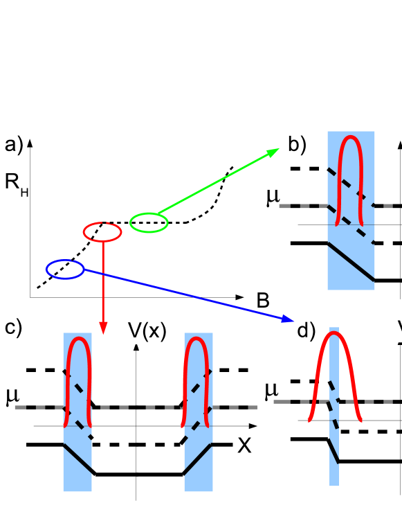
Figure 1: (Color online) (a) Schematic picture of the Hall resistance as a function of $B$. (b)-(d) Corresponding potentials (black solid lines), Landau levels (dashed lines), and wave functions (red solid lines). Here $\mu$ (gray solid lines) is the Fermi energy at equilibrium. The ellipses in (a) indicate the interval in $B$ where the incompressible strips become well-developed (b), washed out (c), or leaky (d). The actual calculations considering realistic structures can be found in Refs. [22, 24, 17]

together with the Hall resistance. There is a steep potential variation in incompressible strips, where the Fermi energy falls in between two consecutive Landau levels. If the incompressible strip is well-developed and larger than the wave extent, the quantized Hall effect is observed [Fig. 1(b)]. However, if the strip width $W_{\rm IS}$ becomes comparable with the wave extent (or the magnetic length ($\ell=\sqrt{\hbar/eB}$) for the lowest Landau level) [Fig. 1(c)] the strip loses its incompressibility, and partitioning between channels becomes possible. Thus, it is possible to observe interference. This case is called as the “leaky” incompressible state, which can be accurately determined by taking into account the collision broadened Landau level width and the extent of the wave function. Once the strip becomes even smaller than the wave extent, the classical Hall effect is observed [23] as shown in Fig. 1(d). Altogether, interference can be observed at the lower end of the quantized Hall plateau.

We calculate of the electron density and the electrostatic potential at the layer of the 2DES self-consistently [24] by using the structural information from Goldman [5]. The dopant density, location of the interface for the 2DES, and the dielectric constant $\kappa$ (= 12.4 for GaAs/AlGaAs) are used as the input to calculate the total potential from $V(\vec{r})=V_{\rm conf}(\vec{r})+V_{\rm int}(\vec{r})$, where the confinement potential $V_{\rm conf}(\vec{r}=(x,y,z))$ is composed of (i) the potential generated by surface pattern (corresponding to trench-gating [18]), (ii) donors, and (iii) surface charges. The interaction potential is calculated from the electron density $n_{el}$ by solving the Poisson equation,

$$V_{\rm int}(\vec{r})=\frac{2e^{2}}{\kappa}\int n_{\rm el}(\vec{r}^{\prime})K(\vec{r};\vec{r}^{\prime})d\vec{r}^{\prime},$$ (1)

where the kernel $K(\vec{r};\vec{r}^{\prime})$ takes into account the imposed boundary conditions. The explicit kernels considering different boundary conditions can be found in Refs. [22, 17] and references therein. The electron density is calculated within the Thomas-Fermi approximation from

$$n_{\rm el}(\vec{r})=\int dE\,D(E;\vec{r})f(V(\vec{r}),E,T,\mu),$$ (2)

where $D(E;\vec{r})$ is the density of states, and the Fermi occupation function $f(V(\vec{r}),E,T,\mu)$ depends on the chemical potential $\mu$ and temperature $T$. The above equations are solved self-consistently on a uniform 3D grid with open boundary conditions.

It is important to note the advantages and constraints of the applied approximations. As a general note, the number of electrons is very large (of the order of $10^{3}$), so that semiclassical or density-functional-type approximations become reasonable in order to obtain a qualitative estimation for the positions and the widths of the current carrying channels. Their exact properties require formidable numerical approaches that are beyond the scope of this work.

The magnetic field effects are included in our static calculations via the approximation of Landau-quantized density of states, although the wave functions should also depend on the position according to the total potential. However, this approximation can be justified for different regimes of compressibility. First, in compressible systems the external potential is well screened (for instance, similar to the potential at the center of Fig. 1(d), so that the total potential is constant. Hence, the Landau wave functions are not modified at all, but the energy eigenvalues are shifted. Secondly, in incompressible systems the total potential varies linearly, and hence the wave functions preserve the Landau form; only their center coordinates are shifted slightly (less than the magnetic length). At the transition regions the potential may vary with higher-order corrections. However, the next (quadratic) correction also preserves the Landau form, whereas the center coordinate remains unaffected. In total, the corrections to the Landau wavefunction are thus negligible up to the third order, which justifies the practical validity of our approximation in determining the electron density. To compensate for the suppression of the tunneling effects due to the Thomas-Fermi approximation we take into account the finite widths of the Landau wave functions as discussed below.

The exact form of $D(E)$ is essentially determined by the properties of the scattering mechanisms in the presence of strong disorder. These constraints are lifted by the experimental conditions, so that the number of electrons within the interferometer is more than $10^{3}$ and the mobility of the samples is extremely high (typically, $\mu\geq 5\times 10^{6}$ cm²/Vs). Hence, in such samples the Landau level broadening can be neglected: $\Gamma/(\hbar\omega_{c})=\Gamma/(eB/m^{\star})\ll 1$, where $\Gamma$ is the level width and $\hbar\omega_{c}$ is the cyclotron energy. Otherwise, the level broadening has been proven to have an important influence on the (in)compressibility of the system [25].

We point out that the statistical description of a many-particle system by the grand-canonical ensemble assumes that the system is in contact with a reservoir, which can exchange particles with the system and determines the chemical potential. If the system is inhomogeneous, one usually considers a constant electrochemical potential in thermal equilibrium, which, however, is position dependent in the case of an imposed current, i.e., in a (global) non-equilibrium.

To proceed with the calculation to the desired values of $B$ and $T$, we impose periodic boundary conditions and replace the constant density of states in the absence of magnetic fields with a Gaussian-broadened one [17] that takes the quantization due to the magnetic field into account, together with disorder. In this procedure, we first increase $T$ and smear the quantization effects with the Fermi function. Then, we set the desired value for $B$ and decrease $T$ stepwise to its target value. In each iteration step a relative accuracy threshold of $<10^{-6}$ is obtained for the density. This standard calculation scheme has been previously used to describe similar systems successfully [22, 24, 17, 23].

In Fig. 2

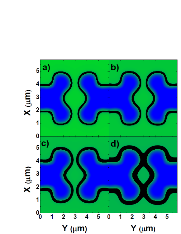
Figure 2: Spatial distribution of the incompressible strips (black) calculated at (a) $B=7.6$ T, (b) $8.0$ T, (c) $8.4$ T, and (d) $8.8$ T at $T=1$ K. It is expected that only at $B=8.0$ T one can observe Aharonov-Bohm oscillations, whereas in the other cases the scattering between the edge-states is prevented (see text).

we show the spatial distribution of incompressible strips at different magnetic fields. The sequence of figures at $B=7.6\ldots 8.8$ T shows that the distance between the incompressible strips decreases, and their width increases, as a function of $B$. It can be expected that at low $B$ when the strips are far apart, the AB oscillations are not present or they are weak, as the wave packet remains in the incoming channel. On the other hand, the strong overlap between the strips at $B=8.8$ T suggests suppression as well – now due to the complete transport of the wave packet to the other channel. Interference would require clean splitting (partitioning) of the wave function between the channels. To confirm this phenomenological suggestion, and to study the effects of the channel distance and width on the conductance, we focus now on realistic modeling of current channels along the incompressible strips. This is followed by a dynamical study on the electron transport in the device. As the core outcome we can qualitatively describe the interference intervals depending on the system parameters such as temperature, sample geometry, and heterostructure properties.

Before introducing the model for dynamics, a brief discussion about the direction of the current along the incompressible strips is in order. It is well known that the current-carrying states in a QH device result from the Landau-level quantization followed by level bending at the edges where the Fermi energy crosses the levels. Thus, the equilibrium transport takes place through the chiral edge states, i.e., with different current directions at opposite edges, and the net current is zero. In transport experiments (including interference experiments), however, an external current is imposed and a Hall (electrochemical) potential difference – with the same slope – develops between two opposing edges [26]. This potential drop at the incompressible strips, that confines the external current in those regions, has been shown in several experiments [27, 28, 29]. In the following we utilize this picture in the transport calculations, so that the electrons flow to the same direction along the opposite channels.

3 Electron transport

The channels are modeled by a 2D potential profile consisting of two curved pipes following the shape of the incompressible strips in Fig. 2. The potential minima of the channels are shown as solid lines in Fig. 3. The distance between the left and right parts is varied such that at the two encountering points (bottom and up) the distance between the potential minima is $d=0\ldots 1$ (in atomic units). It is important to note that the channels are genuinely 2D according to the real device, and their cross sections have a Gaussian form $V_{\rm cross}\approx-V_{0}\,e^{-s^{2}/c^{2}}$, where $s$ is the coordinate perpendicular to the channel, $V_{0}=20$ is the channel depth, and $c=0.2$ is the width parameter which is varied. The choice of a Gaussian profile is justified by considering the magnetic (parabolic) confinement, which is close to a Gaussian form at the bottom of the channel. On the other hand, in the upper part of the channel the selected profile allows “leaking” of the electron flow according to the experiment (see above).

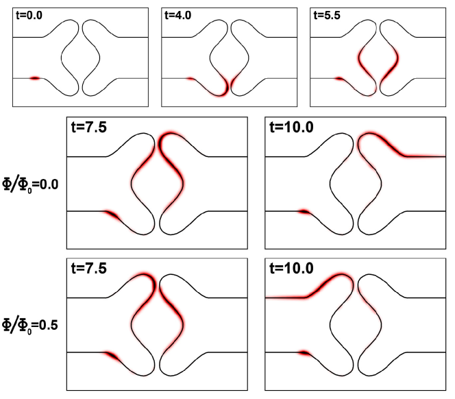
Figure 3: Snapshots of the electron density in a model for the Aharonov-Bohm interferometer. The two lowermost rows correspond to zero flux and half a flux quantum, respectively.

As an initial condition we set a single-electron wave packet in the lower-left corner of the device and, in order to emulate a source-drain voltage, we accelerate the wave packet using a linear potential with slope $V_{1}=-0.2V_{0}$ along the channel, which leads to an initial velocity of $\sim 3.3$ a.u. We monitor the density and the current density during the time propagation until we find back-scattering form the upper left and right corners of our finite simulation box. In this way, we guarantee the correct direction of the current along the incompressible strips (see the discussion above). The conductance as a function of the magnetic field, the channel distance, and the channel width is estimated by calculating the probability $N_{r}$ to find the electron in the upper-right corner within the restricted simulation time (see Ref. [3] for details). We made the time propagation by using the fourth order Taylor expansion of time evolution operator to the single-electron wave function in a 2D real-space grid with the octopus code package [30].

We emphasize that in contrast to the real interferometer (see Fig. 2), where both the channel width and their mutual distance (i.e., the spatial distribution of the incompressible strips) is determined by the magnetic field itself, we let in our model the magnetic field affect only the flux but not the distribution of the channels. However, for each set of calculations, respectively, the width and distance are changed through the model parameters given just above.

In our transport simulations we monitor electron dynamics as a function of a magnetic flux added to the background magnetic field (the latter generating the incompressible strips). In Fig. 3 we show snapshots of the electron density at different times. Here we apply relative fluxes $\Phi/\Phi_{0}=0$ and 0.5, respectively. In the beginning (see the uppermost row) differences in density between these two cases are not visible, so only the other case is plotted. Later on, however, we find a drastic difference between the two cases: whereas zero flux leads to transport to the right (second row), a flux corresponding to half a flux quantum yields strong current to the left (third row). Thus, by exploiting the AB effect, our device is almost completely tunable with respect to the current direction at the ouput (left or right).

To analyze the transport quantization in more detail, we plot in Fig. 4

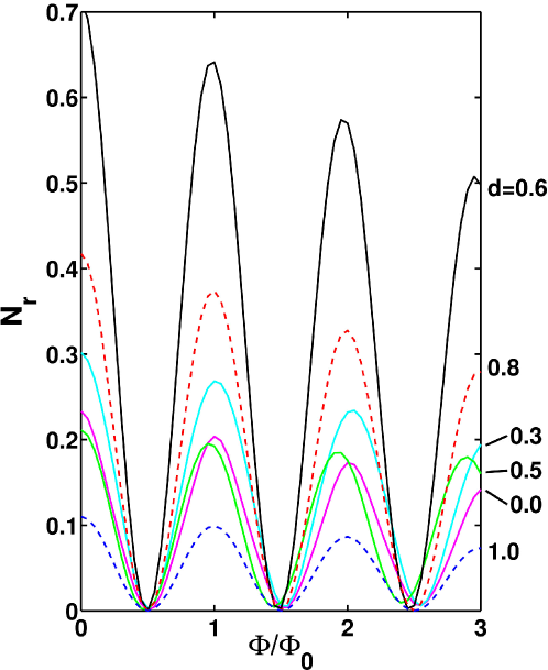
Figure 4: Estimated conductance $N_{r}$ as a function of the magnetic flux in the model interferometer with different distances between the channels.

the conductance – corresponding here to the electron density transferred to the top of the right channel – as a function of the magnetic flux, and for different distances between the channels. We find clear and smooth AB oscillations having exactly the expected periodicity. It is noteworthy that in all cases the interchannel transport is completely blocked at $\Phi/\Phi_{0}=k/2$, where $k$ is an odd integer.

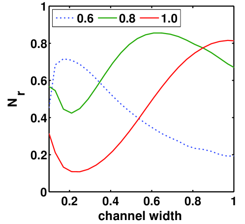
Figure 5: Estimated conductance $N_{r}$ at zero magnetic field as a function of the channel width parameter $c$ for different distances ($d$) between the channels.

An interesting feature in Fig. 4 is the fact that the channel distance has an optimal distance $d\sim 0.6$ when the AB oscillation amplitude is maximized. At smaller (solid lines) and larger (dashed lines) values of $d$ the amplitude is decreased. We find that the optimal distance corresponds to a case when approximately a half of the density is transferred to the right channel at the first (lower) intersection, i.e., the partitioning is equal. Therefore, at the second (upper) intersection we find clear AB interference due to the phase difference of the optimally partitioned electrons that enclose the given flux. Our results agree with the behavior in the AB oscillation strength observed in real AB interferometers [31, 32]. We note, however, that as demonstrated in Fig. 5, the optimal distace depends on the channel width $c$ in a nontrivial fashion – apart from the large-$c$ limit showing clear suppression of the amplitude. However, it seems that half-half partitioning of the density distribution at the first (bottom) point of encounter always leads to a relatively high amplitude of the AB oscillation. A complete quantitative comparison with experiments would require an accurate determination of the system geometry as a function of the magnetic field.

4 Summary

To summarize, we have performed static and dynamical simulations on Aharanov-Bohm interferometers starting from real device parameters. First, the electron density and the spatial distribution of the incompressible strips have been obtained self-consistently within the Thomas-Fermi approximation. These calculations already suggest that interference can take place only if the incompressible strips become leaky, namely not strictly compressible or incompressible, and come close to each other, so that partitioning of the electron current can take place. These phenomenological considerations have then been qualitatively confirmed in the second part of the study, where we time-propagate an electronic wave function injected in the channel with tunable parameters. We observe distinct Aharonov-Bohm oscillations, whose amplitude strongly depends on both the mutual distance between the transport channels and their width. In particular, there is an optimal distance yielding maximum oscillation amplitudes. At magnetic fields corresponding to half-integer flux quanta the suppression of interchannel transport is complete. Taken together, we are able to provide a proof-of-concept for the determination of interference patterns in realistic Aharonov-Bohm interferometers in the quantum Hall regime.

References

References

- [1]
- [2] Y. Aharonov and D. Bohm, Phys. Rev. 115, 485 (1959).
- [3] V. Kotimäki and E. Räsänen, Phys. Rev. B 81, 245316 (2010).
- [4] M. Avinun-Kalish, M. Heiblum, O. Zarchin, D. Mahalu, and V. Umansky, Nature 436, 529 (2005).
- [5] F. E. Camino, W. Zhou, and V. J. Goldman, Phys. Rev B 72, 155313 (2005).
- [6] N. Ofek, A. Bid, M. Heiblum, A. Stern, V. Umansky, and D. Mahalu, Proceedings of the National Academy of Science 107, 5276 (2010).
- [7] M. D. Godfrey, P. Jiang, W. Kang, S. H. Simon, K. W. Baldwin, L. N. Pfeiffer, and K. W. West, ArXiv e-prints (2007), 0708.2448.
- [8] D. T. McClure, Y. Zhang, B. Rosenow, E. M. Levenson-Falk, C. M. Marcus, L. N. Pfeiffer, and K. W. West, Phys. Rev. Lett. 103, 206806 (2009).
- [9] Y. Zhang, D. T. McClure, E. M. Levenson-Falk, C. M. Marcus, L. N. Pfeiffer, and K. W. West, Phys. Rev. B 79, 241304 (2009).
- [10] M. Büttiker, Phys. Rev. Lett. 57, 1761 (1986).
- [11] B. Rosenow and B. I. Halperin, Phys. Rev. Lett. 98, 106801 (2007).
- [12] A. Siddiki, ArXiv e-prints (2010), 1006.5012.
- [13] I. Neder, M. Heiblum, Y. Levinson, D. Mahalu, and V. Umansky, Phys. Rev. Lett. 96, 016804 (2006).
- [14] S. Ihnatsenka and I. V. Zozoulenko, Phys. Rev. B 77, 235304 (2008).
- [15] P. V. Lin, F. E. Camino, and V. J. Goldman, Phys. Rev. B 80, 125310 (2009).
- [16] A. Weichselbaum and S. E. Ulloa, Phys. Rev. E 68, 056707 (2003).
- [17] S. Arslan, E. Cicek, D. Eksi, S. Aktas, A. Weichselbaum, and A. Siddiki, Phys. Rev. B 78, 125423 (2008).
- [18] E. Cicek, A. I. Mese, M. Ulas, and A. Siddiki, Physica E 42, 1095 (2010).
- [19] B. I. Halperin, Phys. Rev. B 25, 2185 (1982).
- [20] D. B. Chklovskii, B. I. Shklovskii, and L. I. Glazman, Phys. Rev. B 46, 4026 (1992).
- [21] B. Kramer, S. Kettemann, and T. Ohtsuki, Physica E 20, 172 (2003).
- [22] A. Siddiki and R. R. Gerhardts, Phys. Rev. B 70, 195335 (2004).
- [23] D. Eksi, O. Kilicoglu, O. Göktas, and A. Siddiki, Phys. Rev. B 82, 165308 (2010).
- [24] A. Siddiki and F. Marquardt, Phys. Rev. B 75, 045325 (2007).
- [25] A. Struck, B. Kramer, T. Ohtsuki, and S. Kettemann, Phys. Rev. B 72, 035339 (2005).
- [26] K. Güven and R. R. Gerhardts, Phys. Rev. B 67, 115327 (2003).
- [27] E. Ahlswede, P. Weitz, J. Weis, K. von Klitzing, and K. Eberl, Physica B 298, 562 (2001).
- [28] E. Ahlswede, J. Weis, K. von Klitzing, and K. Eberl, Physica E 12, 165 (2002).
- [29] F. Dahlem, E. Ahlswede, J. Weis, and K. von Klitzing, Phys. Rev. B 82, 121305 (2010).
- [30] M. A. L. Marques, A. Castro, G. F. Bertsch, A. Rubio, Comput. Phys. Commun. 151, 60 (2003); A. Castro, H. Appel, M. Oliveira, C. A. Rozzi, X. Andrade, F. Lorenzen, M. A. L. Marques, E. K. U. Gross, and A. Rubio, Phys. Stat. Sol. (b) 243, 2465 (2006).
- [31] P. Roulleau, F. Portier, D. C. Glattli, P. Roche, A. Cavanna, G. Faini, U. Gennser, and D. Mailly Phys. Rev. B 76, 161309(R) (2007).
- [32] L. V. Litvin, H.-P. Tranitz, W. Wegscheider, and C. Strunk, Phys. Rev. B 75, 033315 (2007).