Bifurcations in the optimal elastic foundation for a buckling column

Abstract

We investigate the buckling under compression of a slender beam with a distributed lateral elastic support, for which there is an associated cost. For a given cost, we study the optimal choice of support to protect against Euler buckling. We show that with only weak lateral support, the optimum distribution is a delta-function at the centre of the beam. When more support is allowed, we find numerically that the optimal distribution undergoes a series of bifurcations. We obtain analytical expressions for the buckling load around the first bifurcation point and corresponding expansions for the optimal position of support. Our theoretical predictions, including the critical exponent of the bifurcation, are confirmed by computer simulations.

1 Introduction

Buckling is a common mode of mechanical failure [1], and its prevention is key to any successful engineering design. As early as 1759, Euler [2] gave an elegant description of the buckling of a simple beam, from which the so-called Euler buckling limit was derived. Works which cite the goal of obtaining structures of least weight stable against buckling can be found throughout the literature [3, 4, 5, 6, 7], and much understanding has been gained on optimal structural design [1, 8, 9]. Designs of ever increasing complexity have been analysed and recent work suggested that the optimal design of non-axisymmetric columns may involve fractal geometries [10, 11]. With the development of powerful computers, more and more complicated structures can be designed with optimised mechanical efficiency. However, understanding and preventing buckling remains as relevant as ever.

In this paper, we consider a simple uniform elastic beam, freely hinged at its ends and subjected to a compressive force and therefore vulnerable to buckling. However, in contrast to Euler’s original problem, we specify that the beam is stabilized by restoring forces, perpendicular to its length, which are provided by an elastic foundation (as illustrated in figure 1). This represents a simple and practical method of protecting against buckling instabilities.

In the simplest case figure 1, we can imagine this elastic foundation as a finite collection of linear springs at points along the beam. Each has a spring constant, and so provides a restoring force at this point, proportional to the lateral deflection of the beam. More generally, the elastic foundation could be distributed as a continuous function along the length of the beam, rather than being concentrated into discrete springs (figure 1). In this case, there is a spring constant per unit length, which may vary along the beam.

We are interested in optimising this elastic support, and so we need to specify a cost function for it. This we take to be the sum of the spring constants (if there are a discrete collection of springs) or the integral over the spring constant per unit length along the beam (if the elastic foundation is continuous). By choosing the optimal distribution of these spring constants, we wish to find the minimum cost of elastic support which will protect against buckling under a given compressive load (or equivalently, the distribution of an elastic support of fixed cost which will support the maximum force).

The optimal position of one or two deformable or infinitely stiff supports have been studied in the literature (see for example Ref. [12] and references therein), and general numerical approaches established for larger numbers of supports [12]. However, in the present paper, we consider the general case where any distribution of support is in principle permitted.

A perturbation analysis shows that in the limit of weak support strength, the optimal elastic foundation is a concentrated delta-function at the centre of the beam, but when stronger supports are permitted, we show that the optimal solution has an upper bound on the proportion of the beam that remains unsupported. In this sense, the optimum distribution becomes more uniform for higher values of support strength. To tackle the problem in more detail, we develop a transfer matrix description for the supported beam, and we find numerically that the optimal supports undergo a series of bifurcations, reminiscent of those encountered in iterated maps. However, we are only able to proceed a limited distance in the parameter space and we are unable to explore for more complex behaviour (for example, any possible signature of chaos [13]).

We obtain analytic expressions for the buckling load in the vicinity of the first bifurcation point and a corresponding series expansion for the optimal placement of elastic support. Following this optimization we show that a mathematical analogy between the behaviour exhibited in this problem and that found in Landau theory of second order phase transitions[14] exists. However, the analogue of free energy is non-analytic, while in Landau theory it is a smooth function of the order parameter and the control variable. Our results, including critical exponents are confirmed by computer simulations, and should provide a basis for future analysis on higher order bifurcations.

2 Theory

A slender beam of length $L$, hinged at its ends, under a compressive force $F$, is governed by the Euler-Bernoulli beam equation [1]:

$$EI\frac{d^{4}\tilde{y}}{d\tilde{x}^{4}}+F\;\frac{d^{2}\tilde{y}}{d\tilde{x}^{2}}+q(\tilde{x})=0,$$ (1)

where $E$ is the Young modulus of the beam, $I$ is the second moment of its cross sectional area about the neutral plane, $\tilde{y}$ is the lateral deflection, $\tilde{x}$ the distance along the beam and $q(\tilde{x})$ is the lateral force applied per unit length of beam. The beam is freely hinged at its end points and therefore the deflection satisfies $\tilde{y}=\tilde{y}^{\prime\prime}=0$ at $\tilde{x}=0$ and $L$.

If the lateral force is supplied by an elastic foundation, which provides a restoring force proportional to the lateral deflection, then through rescaling we introduce the following non-dimensional variables $x=\pi\tilde{x}/L$, $y=\pi\tilde{y}/L$, $f=FL^{2}/(EI\pi^{2})$ and $\rho=qL^{4}/(EI\pi^{4}\tilde{y})$. Eq. (1) becomes

$$\frac{d^{4}y}{dx^{4}}+f\;\frac{d^{2}y}{dx^{2}}+\rho(x)y=0\ \ \ {\rm for}\ \ \ x\in(0,\pi),$$ (2)

where $y(0)=y(\pi)=y^{\prime\prime}(0)=y^{\prime\prime}(\pi)=0$ and $\rho(x)$ represents the strength of the lateral support (for example the number of springs per unit length) at position $x$.

We are always interested in the minimum value $f_{\min}$ of $f$ that leads to buckling [in other words, the smallest eigenvalue of Eq. (2)]. For the case of no support ($\rho=0$), the possible solutions to Eq. (2) are $f\in\mathbb{Z}^{+}$, and so buckling first occurs when $f=1$.

Lateral support improves the stability (increasing the minimum value of the applied force $f$ at which buckling first occurs), but we imagine that this reinforcement also has a cost. In particular, for a given value of

$$m\equiv\int\rho(x)\;dx,$$ (3)

we seek the optimal function $\rho(x)$ which maximises the minimum buckling force $f_{\min}$.

The simplest choice we can imagine is that $\rho$ takes the uniform value $m/\pi$, so that the form of deflection is $y(x)\propto\sin kx$, for some integer $k$, which represents a wavenumber.

This leads immediately to the result that in this case

$$f_{\min}=\min_{k\in\mathbb{Z}}\left[k^{2}+\frac{m}{\pi k^{2}}\right].$$ (4)

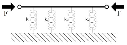
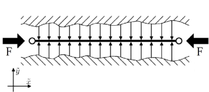
Figure 1: Schematic of a slender beam with elastic support, loaded under compression force $F$. (a) shows the case where the lateral restoring force per unit length along the beam $q(\tilde{x})$ is provided by linear springs of spring constant $\{k_{i}\}$ at discrete points $\{\tilde{x}_{i}\}$, so that $q(\tilde{x})=\sum_{i=1}^{4}k_{i}\delta(\tilde{x}-\tilde{x}_{i})\tilde{y}/L$. (b) shows schematically the case where there is a continuous support: the lengths of the arrows indicate the local spring constant.

Eq. (4) has a physical interpretation: the first term comes from the free buckling of the column which is most unstable to buckling on the longest allowed length scales (i.e. the smallest values of $k$), as demonstrated by Euler. The second term represents the support provided by the elastic foundation, which provides the least support at the shortest length scales (largest values of $k$). The balance between these two terms means that as $m\rightarrow\infty$, the uniformly supported column buckles on a length scale of approximately

$$l_{\rm eff}\approx(\pi/m)^{1/4}\ \ \ {\rm as}\ \ \ m\rightarrow\infty,$$ (5)

and can support a load

$$f_{\rm uni}\sim 2\sqrt{m/\pi}.$$ (6)

Now, although a uniform elastic support is easy to analyse, it is clear that this is not always optimal. Consider the case where $m$ is very small, so that $\rho$ provides a small correction in Eq. (2). In this case, the eigenvalues remain well-separated, and we can treat the equation perturbatively: let

$$y=y_{0}\sin x+y_{1}(x)\ \ \ {\rm and}\ \ \ f=1+f_{1},$$ (7)

then from Eq. (2), if we multiply through by $\sin x$ (the lowest unperturbed eigenfunction) and integrate, we have to leading order:

$$\int_{0}^{\pi}\left\{\sin x\left[\frac{d^{4}y_{1}}{dx^{4}}+\frac{d^{2}y_{1}}{dx^{2}}\right]+y_{0}\sin^{2}x\left[\rho-f_{1}\right]\right\}{\rm d}x=0.$$ (8)

Repeated integrations by parts with the boundary conditions $y_{1}^{\prime\prime}=0$ at $x=0,\pi$ establishes the self-adjointness of the original operator, and we arrive at

$$f_{1}=\frac{2}{\pi}\int_{0}^{\pi}\rho(x)\sin^{2}x\;{\rm d}x.$$ (9)

We therefore see that in the limit $m\rightarrow 0$, the optimal elastic support is $\rho(x)=m\delta(x-\pi/2)$, and for this case, $f_{\min}=1+(2m/\pi)+O(m^{2})$.

The requirement for optimal support has therefore concentrated the elastic foundation into a single point, leaving the remainder of the beam unsupported.

3 Transfer Matrix formulation

In order to proceed to higher values of $m$ in the optimization problem, we assume that there are $N-1$ discrete supports at the positions $\{x_{n}\}$, with corresponding set of scaled spring constants $\{\beta_{n}\}$, adding up to the total $m$:

$$\rho(x)=\sum_{n=1}^{N-1}\beta_{n}\delta(x-x_{n})$$ (10)

$$m=\sum_{n=1}^{N-1}\beta_{n}\;$$ (11)

These discrete supports divide the beam into $N$ (not necessarily equal) segments, and for convenience in later calculations, we also define the end points as $x_{0}\equiv 0$ and $x_{N}\equiv\pi$.

For each segment of the beam given by $x_{n}<x<x_{n+1}$, the Euler-Bernoulli equation (2) can be solved in the form

$$y(x)=A_{n}\sin[f^{1/2}(x-x_{n})]+B_{n}\cos[f^{1/2}(x-x_{n})]$$

$$+C_{n}(x-x_{n})+D_{n}.$$ (12)

If we integrate Eq. (2) over a small interval around $x_{n}$, we find that,

$$y\left(x_{n}^{+}\right)=y\left(x_{n}^{-}\right),\quad y^{\prime}\left(x_{n}^{+}\right)=y^{\prime}\left(x_{n}^{-}\right),$$

$$y^{\prime\prime}\left(x_{n}^{+}\right)=y^{\prime\prime}\left(x_{n}^{-}\right),$$

$$y^{\prime\prime\prime}\left(x_{n}^{+}\right)-y^{\prime\prime\prime}\left(x_{n}^{-}\right)+\beta_{n}y\left(x_{n}\right)=0,$$ (13)

where $x_{n}^{+}$ and $x_{n}^{-}$ are values infinitesimally greater and less than than $x_{n}$ respectively. Defining $\mathbf{v}_{n}\equiv(A_{n},B_{n},C_{n},D_{n})^{T}$, these continuity constraints on the piecewise solution of Eq. (12) can be captured in a transfer matrix

$$\mathbf{v}_{n}=T_{n}\cdot\mathbf{v}_{n-1},$$ (14)

where $T_{n}$ is given by

$$\left(\begin{array}[]{cccc}\frac{\beta_{n}}{f^{3/2}}S_{n}+K_{n}&\frac{\beta_{n}}{f^{3/2}}K_{n}-S_{n}&\frac{\beta_{n}}{f^{3/2}}\Delta x_{n}&\frac{\beta_{n}}{f^{3/2}}\\ S_{n}&K_{n}&0&0\\ -\frac{\beta_{n}}{f}S_{n}&-\frac{\beta_{n}}{f}K_{n}&1-\frac{\beta_{n}}{f}\Delta x_{n}&-\frac{\beta_{n}}{f}\\ 0&0&\Delta x_{n}&1\end{array}\right)$$ (15)

and

$$\Delta x_{n} \equiv x_{n}-x_{n-1}$$

$$S_{n} \equiv \sin[f^{1/2}(x_{n}-x_{n-1})],$$

$$K_{n} \equiv \cos[f^{1/2}(x_{n}-x_{n-1})].$$

At the two end-points at $x=0$, $\pi$, we have the boundary conditions that $y$ and $y^{\prime\prime}$ vanish, which leads to the following four conditions

$$B_{0}=D_{0} = 0$$ (16)

$$A_{N-1}S_{N}+B_{N-1}K_{N} = 0$$ (17)

$$C_{N-1}(x_{N}-x_{N-1})+D_{N-1} = 0.$$ (18)

If we now define a matrix

$$\mathbf{R}=T_{N-1}T_{N-2}\ldots T_{2}T_{1}$$ (19)

then Eqs. (16-18) lead to

$$\mathbf{M}\cdot\left(\begin{array}[]{c}A_{0}\\ C_{0}\end{array}\right)=0$$ (20)

where

$$\mathbf{M}\equiv\left(\begin{array}[]{cc}R_{11}S_{N}+R_{21}K_{N}&R_{13}S_{N}+R_{23}K_{N}\\ (\Delta x_{N})R_{31}+R_{41}&(\Delta x_{N})R_{33}+R_{43}\end{array}\right)$$ (21)

For the beam to buckle, there needs to be non-zero solutions for $A_{0}$ and/or $C_{0}$. Therefore, the determinant of $\mathbf{M}$, which is a function of $f$, must go to zero. The smallest $f$, $f_{\min}$, at which $\det(\mathbf{M})=0$, gives the maximum compression tolerated by the beam and its support. The task, thus, is to find the set of $\{\beta_{n}\}$ and $\{x_{n}\}$ which maximise $f_{\min}$.

4 Equally spaced, equal springs

Any definite choice of $\rho(x)$ provides a lower bound on the maximum achievable value of $f_{\min}$, so before discussing the full numerical optimization results on $\rho$, we consider here a simple choice of $\rho$ which illuminates the physics.

Figure 2: Value of $f_{\min}$ for $\rho$ constant (dashed line), and for equally spaced, equally strong delta functions ($N$ is the number of intervals, so $N-1$ is the number of delta-functions).

Suppose that $\rho$ consists of equally spaced, equally strong delta-functions:

$$\rho_{N}(x)=\sum_{n=1}^{N-1}\frac{m}{N-1}\delta(x-\pi/n).$$ (22)

The value of $f_{\min}$ can be found by a straight-forward calculation for each value of $m$, using the transfer matrix formulation above. The results are plotted in figure 2, and we see that in general, it is better to concentrate the elastic support into discrete delta functions, rather than having a uniform elastic support. However, it is important to choose the appropriate number of delta functions: if the number is too few, then there will always be a buckling mode with $f=N^{2}$ which threads through the comb of delta functions without displacing them. However, apart from this constraint, it appears to be advantageous to choose a smaller value of $N$; in other words, to concentrate the support.

5 Numerical optimization of the support

Figure 3: Results of the restricted optimization, obtaining the set $\{x_{n}\}$ with constant $\beta_{n}=m/(N-1)$.

Before we look at the general optimization problem where we will seek the optimal set of $\{x_{n}\}$ and $\{\beta_{n}\}$ for a given cost, we investigate a simplified problem to give us further insight into the nature of the problem. We set

$$\beta_{n}=\frac{m}{N-1}\quad\forall\quad n$$ (23)

and then find the set $\{x_{n}\}$ which maximises $f_{min}$. The results obtained from an exhaustive search are shown in figure 3, where we find two bifurcation points in the range $0<m\leq 40.$ The critical exponent of each has been obtained through simulation as,

$$\alpha_{1} = 0.5\pm 0.01,$$ (24)

$$\alpha_{2} = 0.49\pm 0.03,$$ (25)

for the first and second bifurcation respectively. Figure 4 shows the data from which the exponents are taken, where values of $m_{0}$ and $x_{0}$ used are,

$$m_{0}=5.09,\;26.99$$ (26)

$$x_{0}=0.5,\;0.281$$ (27)

for the first and second bifurcation respectively. The value of $x_{0}$ for the lower branching event at $m=26.99$ is related to the upper branch by symmetry about the midpoint of the beam. As discussed previously, the optimal solution must split further at higher values of $m$. We hypothesize that within this restricted problem these splits will take the form of bifurcations similar in nature to those found here.

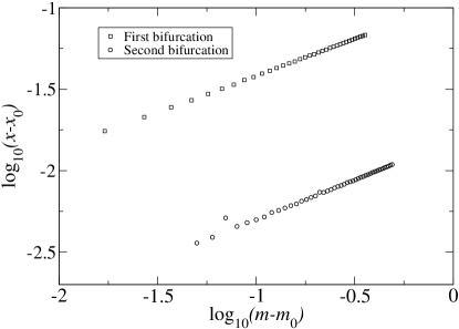
Figure 4: Showing the critical exponents for the first and second bifurcation in the restricted problem of $\beta_{n}=m/(N-1)$.

Now we turn to the full optimization problem, where the values $\{\beta_{i}\}$ as well as the positions $\{x_{i}\}$ of the supports may vary. Using the transfer matrix formulation, we seek the optimal elastic support consisting of delta functions. Figure 5 shows the best solutions, found from an exhaustive search of four delta functions ($N=5$), up to $m=50$. We see in figure 4 that there are two bifurcation events, and one coalescence of the branches. Because the optimal solution cannot contain long intervals with no support (see section 7 below), we expect that if continued to larger values of $m$ and $N$, a series of further bifurcation events would lead to a complex behaviour which would eventually fill the interval with closely spaced delta functions as $m\rightarrow\infty$.

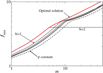
Figure 5: Value of $f_{\min}$ for the optimal form of $\rho(x)$ and also for comparison $\rho$ constant, and for equally spaced, equally strong delta functions.

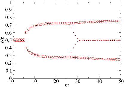
Figure 6: Position of optimal springs as a function of $m$. The area of each circle is proportional to the strength $\beta_{i}$ of the relevant support, with the total area of all the circles at each value of $m$ chosen to be a constant, independent of $m$.

6 First branch point

Numerical results (figure 5) indicate that although a single delta function at $x=\pi/2$ is the optimal form for $\rho$ in the limit $m\rightarrow 0$, at some point the optimal support bifurcates.

It is clear that this first bifurcation must happen at $f=4$, since this represents the excitation of the first anti-symmetric buckling mode in the unsupported beam, and the delta function at $x=\pi/2$ provides no support against this mode. Although the value of $f$ at this first branch point is clear, neither the value of $m$ at which it occurs, nor the nature of the bifurcation are immediately obvious.

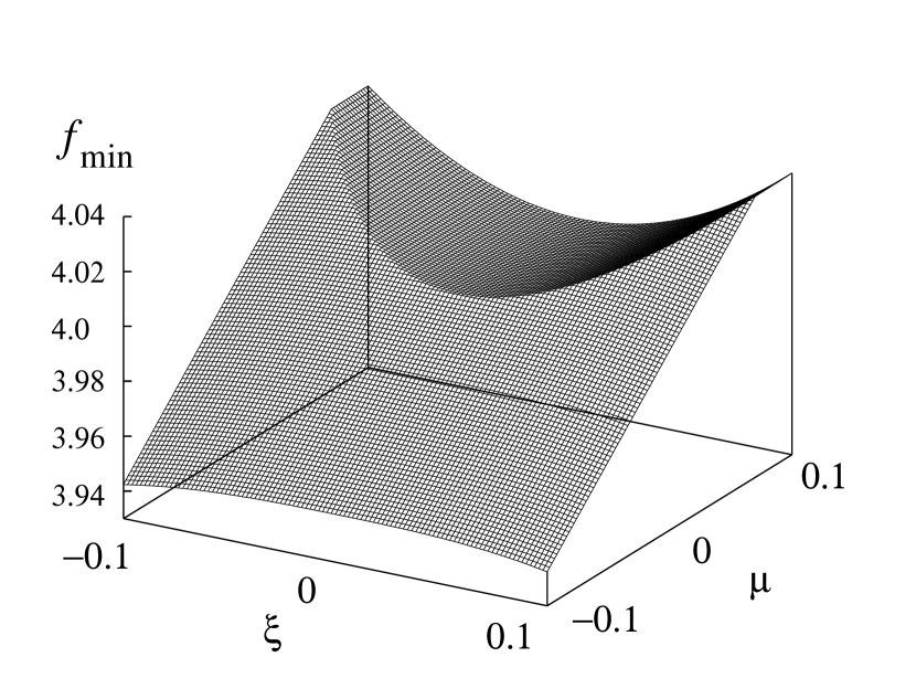
Figure 7: Three dimensional plot of $f_{\min}$ as a function of the position parameter $\xi$ and $\mu\equiv m-(16/\pi)$.

In order to clarify the behaviour at this first branch point, we perform a perturbation expansion: Let us suppose that $N=3$ and

$$\rho(x)=\frac{m}{2}\delta\left(x-\frac{\pi}{2}+\xi\right)+\frac{m}{2}\delta\left(x-\frac{\pi}{2}-\xi\right),$$ (28)

where $\xi$ and $-\xi$ are clearly equivalent, and we will quote only the positive value later. Thus $\{x_{0},x_{1},x_{2},x_{3}\}$ are given by $\{0,\pi/2-\xi,\pi/2+\xi,\pi\}$ and $\beta_{1}=\beta_{2}=m/2$.

We wish to evaluate the matrix $\mathbf{M}$ in Eq. (21) and seek the smallest $f$ giving a zero determinant. On performing a series expansion of the determinant for $f$ near $4$, we find that the critical value of $m$ is $16/\pi$. Furthermore, if we define small quantities $\mu$ and $\xi$ through

$$m=\frac{16}{\pi}+\mu\equiv\frac{16}{\pi}+\mu^{\prime}\epsilon$$ (29)

$$\xi\equiv\xi^{\prime}|\epsilon|$$ (30)

where $\epsilon\ll 1$ and $\xi^{\prime}$ and $\mu^{\prime}$ are order $1$ quantities and

$$f=f(\xi,\mu),$$ (31)

then we can perform a series expansion of $\det(\mathbf{M})$ in the neighbourhood of $\epsilon=0$, to obtain term by term a series expansion for $f$. We find that there are two solutions, $f_{+}$ and $f_{-}$, which correspond to functions $y(x)$ symmetric and anti-symmetric about $x=\pi/2$ respectively:

$$f_{+}=\left[4+\frac{\pi}{6}\mu-\frac{\pi^{2}}{576}\mu^{2}+\frac{\pi^{3}(6-\pi^{2})}{124416}\mu^{3}\right.$$

$$\left.+\frac{\pi^{4}(2\pi^{2}-21)}{11943936}\mu^{4}\right.$$

$$\left.+\frac{\pi^{5}\left(315-15\pi^{2}-\pi^{4}\right)}{4299816960}\mu^{5}+O(\mu^{6})\right]$$

$$+|\xi|\left[0+O(\mu^{5})\right]$$

$$+\xi^{2}\left[\frac{2\pi}{9}\mu+\frac{\pi^{2}}{72}\mu^{2}-\frac{\pi^{3}\left(3+\pi^{2}\right)}{93312}\mu^{3}+O(\mu^{4})\right]$$

$$+|\xi^{3}|\left[-\frac{128}{9\pi}-\frac{40}{27}\mu-\frac{\pi\left(15-\pi^{2}\right)}{486}\mu^{2}+O(\mu^{3})\right]$$

$$+\xi^{4}\left[0+O(\mu^{2})\right]+|\xi^{5}|\left[-\frac{1024}{135\pi}+O(\mu)\right]$$ (32)

$$f_{-}=4+|\xi|\left[0+O(\mu^{5})\right]+\xi^{2}\left[\frac{32}{\pi^{2}}+\frac{2}{\pi}\mu+O(\mu^{4})\right]$$

$$+|\xi^{3}|\left[0+O(\mu^{3})\right]$$

$$+\xi^{4}\left[-\frac{(128\pi^{2}+576)}{3\pi^{4}}-\frac{(8\pi^{2}+72)}{3\pi^{3}}\mu+O(\mu^{2})\right]$$

$$+|\xi^{5}|\left[\frac{512}{3\pi^{3}}+O(\mu)\right].$$ (33)

The final value for $f_{\min}$ in this neighbourhood is then $f_{\min}=\min(f_{+},f_{-})$.

The results are plotted in figure 7, and we see that the behaviour of $f_{\min}$ around the bifurcation point is not analytic, since the transition between the two branches $f_{+}$ and $f_{-}$ leads to a discontinuity in the derivatives of $f_{\min}$. The maximal value of $f_{\min}$ (i.e the optimum we are seeking), occurs for $\xi=0$ when $\mu<0$, and along the locus $f_{+}=f_{-}$ when $\mu>0$.

From Eqs. (32) and (33), this leads to the optimal value of $\xi$ being

$$\xi_{\rm opt}=\begin{cases}\frac{\pi^{3/2}}{8\sqrt{3}}\mu^{1/2}-\frac{\pi^{4}}{864}\mu+O\left(\mu^{3/2}\right)\>&\text{if $\>\mu\geq 0$}\\ 0\>&\text{if $\>\mu<0$}\end{cases}$$ (34)

This is shown in figure 8, together with the regions of the $\mu-\xi$ plane in which $f_{+}$ and $f_{-}$ apply.

Figure 8: Curve shows the locus of optimal values for $\xi$ near the first bifurcation point. This divides the $\xi-\mu$ plane into three regions, in which $f_{\min}$ is given by either Eq. (32) or (33) as indicated.

7 Limit of large support stiffness

The results of our numerical optimisation suggests that the optimum support continues to take the form of a discrete set of delta-functions. Here we investigate the possible form of the optimal support in the limit of large $m$.

As $m$ increases, the optimal distribution function $\rho_{\rm opt}$ must become more evenly distributed over the interval. To see in what sense this is true, we note that the eigenvalue problem for buckling modes given by Eq. (2) can be derived from an energy approach: Suppose that $z(x)$ is any deformation of the beam, then the energy of our system is given [1] by

$$U=\frac{1}{2}\int_{0}^{\pi}\left[\left(\frac{d^{2}z}{dx^{2}}\right)^{2}-f\left(\frac{dz}{dx}\right)^{2}+\rho(x)z^{2}\right]{\rm d}x.$$ (35)

Any deformation $z(x)$ which results in $U[z(x)]<0$ means that the beam will be energetically allowed to buckle under this deflection. Furthermore, the associated value of $f$ which just destabilises the system against this deformation cannot be smaller than the lowest buckling mode $f_{\min}$.

Consider therefore a particular choice for $z(x)$, namely

$$z(x)=\left\{\begin{array}[]{ll}0&x\in(0,x_{1})\\ \sin^{2}\left[\frac{\pi(x-x_{1})}{x_{2}-x_{1}}\right]&x\in(x_{1},x_{2})\\ 0&x\in(x_{2},1)\end{array}\right.,$$ (36)

which vanishes everywhere except on the interval $\Omega=(x_{1},x_{2})$, which is of length $\lambda\equiv x_{2}-x_{1}$. Then Eq. (35), together with the observation above about $f_{\min}$ leads to

$$f_{\rm min}[\rho(x)]\leq\frac{2\pi^{2}}{\lambda^{2}}+\frac{\lambda}{\pi^{2}}\int_{\Omega}\rho(x)\sin^{4}\left[\frac{\pi(x-x_{1})}{\lambda}\right]{\rm d}x.$$ (37)

Trivially, we note from the definition of $\rho_{\rm opt}$, that

$$\forall\rho:f_{\min}[\rho(x)]\leq f_{\min}[\rho_{\rm opt}(x)],$$ (38)

so that from Eqs. (6), (37) and (38), we finally arrive at a condition for how evenly distributed $\rho_{\rm opt}$ must be for large $m$:

$$\forall\Omega:\int_{\Omega}\rho_{\rm opt}(x)\sin^{4}\left[\frac{\pi(x-x_{1})}{\lambda}\right]{\rm d}x\geq\frac{2\pi^{3/2}m^{1/2}}{\lambda}-\frac{2\pi^{4}}{\lambda^{3}}.$$ (39)

A simple corollary of Eq. (39) is that if $\rho_{\rm opt}$ is zero on any interval $\Omega$ of length $\lambda$, then it must be the case that

$$\lambda\leq\pi^{5/4}m^{-1/4}.$$ (40)

The scaling of this length with $m$ is the same as the effective buckling length of a uniformly supported beam discussed earlier.

8 Discussion

The optimal elastic support for our column appears to display complex behaviour: at small values of $m$ the support is a single delta function, and even at large values of $m$, it appears to be advantageous for $\rho(x)$ to be concentrated into discrete delta-functions rather than to be a smooth distribution.

Furthermore, the manner in which the system moves from a single to multiple delta functions is not trivial, and appears to be through bifurcation events. In the full optimization problem we find that the first bifurcation event occurs with critical exponent of one half. Inverting Eq. (34) and substituting it into either Eq. (32) or (33) we find that,

$$f_{\rm min}\approx\begin{cases}4+\frac{32}{\pi^{2}}\xi_{\text{opt}}^{2}-\frac{64\left(2\pi^{2}-9\right)}{3\pi^{4}}\xi_{\rm opt}^{4}\>&\text{if $\>\mu\geq 0$}\\ 4+\frac{\pi}{6}\mu-\frac{\pi^{2}}{576}\mu^{2}\>&\text{if $\>\mu<0$.}\end{cases}$$ (41)

while to leading order,

$$\xi_{\rm opt}=\begin{cases}\frac{\pi^{3/2}}{8\sqrt{3}}\mu^{1/2}\>&\text{if $\>\mu\geq 0$}\\ 0\>&\text{if $\>\mu<0$.}\end{cases}$$ (42)

In this form, the mathematical similarities to Landau theory of second order phase transitions become apparent, with $\xi_{\rm opt}$ playing the role of the order parameter, $\mu$ the reduced temperature and $-f_{\min}$ the free energy to be minimized.

However, there is an important difference. In Landau theory of second order phase transitions, the free energy $F_{\rm lan}$ is assumed to be a power series expansion in the order parameter $\psi$ with leading odd terms missing:

$$F_{\rm lan}=F_{0}+a_{2}\psi^{2}+a_{4}\psi^{4}+...$$ (43)

where $a_{2}\propto(T-T_{c})$, the reduced temperature. In our case, the buckling force $f$ has to be first optimised for even and odd buckling. Thus $-f_{\min}$ (which is the analogue of $F_{\rm lan}$) is a minimum over two intersecting surfaces (figure 7) and so non-analytic at the point of bifurcation.

Nevertheless, the mathematical form of the solution in Eq. (42) is the same, including the critical exponent. Furthermore, our numerical results show that, for the equal support case, the critical exponent $\alpha$ is preserved for the next bifurcation, suggesting that the nature of subsequent bifurcations will also remain the same.

The details of the behaviour for larger values of $m$ is as yet unclear: we speculate that there will be a cascade of bifurcations, as seen in the limit set of certain iterated maps [15]; it remains an open question whether there is an accumulation point leading to potential chaotic behaviour.

Further investigation of this regime may shed light on structural characteristics required to protect more complex engineering structures against buckling instabilities.

9 Acknowledgements

The authors wish to thank Edwin Griffiths for useful discussions. The figures were prepared with the aid of ‘Grace’ (plasma-gate.weizmann.ac.il/Grace), ‘gnuplot’ (http://www.gnuplot.info) and ‘xfig’ (www.xfig.org). Series expansions were derived with the aid of ‘Maxima’ (maxima.sourceforge.net).

References

- [1] Timoshenko S. P. and Gere J. M, Theory of Elastic Stability (McGraw Hill, 1986)
- [2] Euler L., Mem. Acad. Sci. Berlin, 13, 252 (1759)
- [3] Lagrange J.-L, Ouvres de Lagrange, p125-170 (Gauthier Villars, Paris, 1868)
- [4] Cox S. J., Mathematical Intelligencer, 14, 16, (1992)
- [5] Weaver P. M. and Ashby M. F., Prog. Mat. Sci., 41, 61-128 (1997)
- [6] Budiansky B., Int. J. Solids Struct., 36, 3677-3708 (1999)
- [7] Tian Y. S. and Lu T.J., Thin-Walled Structures, 43, 477-498 (2005)
- [8] Cox H. L., The design of structures of least weight, (Pergamon Press, Oxford, 1965)
- [9] Gordon J. E., Structures, (Penguin Books Ltd., 1986)
- [10] Farr R. S., Phys. Rev. E, 76, 046601 (2007)
- [11] Farr R. S. and Mao Y., EPL, 84, 14001, (2008)
- [12] Olhoff N. and Åkesson B., Structural Optimization ,3, 163 (1991)
- [13] Glendinning P., Stability, Instability and Chaos (Cambridge University Press, 1994)
- [14] Landau L. and Lifschitz E.M., Course of theoretical physics vol. 5 (Statistical physics part 1) (Pergamon Press, 1994)
- [15] Feigenbaum M.J., J. Stat. Phys., 19(1), 25, (1978)