Bubble dynamics in double stranded DNA : A Rouse chain based approach

Abstract

We propose a model for the fluctuation dynamics of the local denaturation zones (bubbles) in double-stranded DNA. In our formulation, the DNA strand is model as a one dimensional Rouse chain confined at both the ends. The bubble is formed when the transverse displacement of the chain attains a critical value. This simple model effectively reproduces the autocorrelation function for the tagged base pair in the DNA strand as measured in the seminal single molecule experiment by Altan-Bonnet et. al (Phys. Rev. Lett. 90, 138101 (2003)). Although our model is mathematically similar to the one proposed by Chatterjee et al. (J. Chem. Phys. 127, 155104 (2007)) it goes beyond a single reaction coordinate description by incorporating the chain dynamics through a confined Rouse chain and thus considers the collective nature of the dynamics. Our model also shows that the autocorrelation function is very sensitive to the relaxation times of the normal modes of the chain, which is obvious since the fluctuation dynamics of the bubble has the contribution from the different normal modes of the chain.

I introduction

In 1953 Watson and Crick Watson and Crick (1953) proposed the structure of DNA to be a stable double-stranded helix. The stability comes through the staking interaction and the hydrogen bonding between the base pairs in the opposite strands. But actually this picture represents the equilibrium structure of DNA under physiological conditions. As the interaction energy between these base pairs is only few $k_{B}T$, even at room temperature due to thermal fluctuations locally DNA strand opens up creating what is called “bubbles”. These bubbles have different sizes and lifetimes. The creation and annihilation kinetics of these bubbles is termed as the breathing dynamics. On increasing the temperature or changing the pH these bubbles add up to form larger bubbles and eventually the double stranded DNA denatures.

In recent past single molecule fluorescence correlation spectroscopy (FCS) experiment by Altan-Bonnet et. al Altan-Bonnet et al. (2003) has provided the first quantitative insight to the relaxation kinetics of the breathing mode of the double-stranded DNA. This breathing mode refers to local denaturation and reclosing of the double-stranded structure. In their experiment, two bases of the double-stranded DNA, corresponding to opposite strands are tagged with a fluorophore and a quencher respectively. So when the DNA structure is closed, fluorophore and the quencher are in close proximity and the fluorescence is quenched. But due to thermal fluctuation when the DNA structure opens up creating a bubble, the fluorescence is restored. Hence the base pair fluctuation leads to a fluctuation in fluorescence intensity. This fluctuation in fluorescence intensity is monitored by FCS which determines the characteristic dynamics of the relaxation of dynamic correlations in the fluctuation of base pairs. They introduced a correlation function

$$G(t)=\frac{\left<I(t)I(0)\right>-\left<I(t)\right>\left<I(0)\right>}{\left<I(0)^{2}\right>-\left<I(0)\right>^{2}}$$ (1)

where $I(t)$ is the fluorescent intensity at time $t$. $G(t)$ was found to be multiexponential. Interestingly the correlation function for all the DNA constructs, at all temperatures follow the same universal temporal behavior and when presented as a function of rescaled time they all collapse into a single universal curve $G(t/t_{1/2})$, where $t_{1/2}$ is such that $G(t/t_{1/2})=0.5$. To explain the experimental data they proposed a simple kinetic model in which $G(t/t_{1/2})$ becomes

$$G_{ex}(z)=(1+\frac{mz}{2})erfc(\sqrt{\frac{mz}{2}})-\sqrt{\frac{mz}{\pi}}e^{-\frac{mz}{4}}$$ (2)

where, $z=\frac{t}{t_{1/2}}$ and $m$ is a parameter which is adjusted to $0.328$ to ensure that $G_{ex}(1)=0.5$.

Since this experimental work by Altan-Bonnet et. al, the topic “bubble dynamics” as it is commonly refereed to has received a great deal of theoretical attention. Just few years after this seminal experimental study of the transient time-dependent rupture and re-healing of double stranded DNA, Bicout and Kats Bicout (2004) proposed a kinetic scheme based on two state model (closed or open) of the double stranded DNA. Their formulation gave an analytical expression for the survival probability, correlation function and life time for the bubble relaxation dynamics but formulation did not consider the structure of the double stranded DNA at any level. Very recently Srivastava and Singh Srivastava (2009) proposed a theoretical model where the interaction between the base pairs of the opposite DNA strands is described by Peyard-Bishop-Dauxois (PBD) Bicout (1993) potential and the separation between the base pairs (“y” in their notation) follows a Fokker-Planck equation. Thus only making the interaction realistic but still not taking into account of the dynamics of the chain and restricting to a single relevant dynamical variable (separation “y”) description. In a paper by Jeon, Sung and Ree Jeon (2006) double stranded DNA was modeled as a duplex of semiflexible chains mutually bonded by weak interactions in other words they used an extended worm-like chain model and a Langevin dynamics simulation was performed to examine the size distribution and dynamics of the bubble. Shortly after this Fogedby and Metzler Fogedby and Metzler (2007) came up with a theoretical model for the bubble dynamics . They used the Poland-Scheraga free energy Poland and Scheraga (1966) where the free energy is a function of bubble size $x$. The dynamics of $x$ follows a Langevin equation and the corresponding Fokker-Planck equation is analogous to the imaginary time Schrodinger equation for a particle moving in a Coulomb potential subject to a centrifugal barrier. This mapping enabled them to calculate the correlation function. But the best fit to the long time behavior was obtained only when they considered the dynamics of $x$ in a linear potential. Thus to reproduce the long time data one can merely start with a linear potential but unfortunately it may not fit to the experimental data in the intermediate time range. Interestingly the shortcomings of the Fogedly-Metzler model was pointed out by Chatterjee et. al Chatterjee et al. (2007). They assumed that the distance between fluorophore and the quencher follows an overdamped Langevin equation in a harmonic potential. Although their theory predicts the experimental data reasonably well it does not take into account of the fluctuation of different modes of the DNA strand contributing to the bubble dynamics. A better theory should account for those and actually our model does. In our formulation the DNA-strand is described by a Rouse chain Doi and Edwards (1988); Kawakatsu (2004) confined at both the ends. Transverse displacement of the string accounts for the bubble formation. Naturally our model takes into account of the contribution of different modes of the string to the breathing dynamics.

II Our model

We describe the bubble by a confined Rouse chain Doi and Edwards (1988); Kawakatsu (2004) in a harmonic potential, $V(x)=\frac{1}{2}\kappa R(n)^{2}$, where $R(n,t)$ denotes the position of the $n$th segment of the confined Rouse chain in space and $t$ is the time. In other words the chain is described by a field $R(n,t)$. Because of the thermal fluctuations the bubble undergoes Brownian motion and its time development is described by the equation

$$\zeta\frac{\partial R(n,t)}{\partial t}=k\frac{\partial^{2}R(n,t)}{\partial n^{2}}-\kappa R(n,t)+f(n,t).$$ (3)

In the above, $\zeta$ is the friction coefficient for the $n$th segment and $\kappa$ is the force constant for the confining potential which accounts for the staking interaction between the opposite strands of the DNA molecule.

The fluorescent intensity at time $t$, denoted by $I(t)$ can be written as

$$I(t)=A\theta(R(a,t)-\alpha)$$ (4)

where $R(a,t)$ denotes the position of the $a$th segment in space. Later on we will choose $a$ such that it corresponds to the center of the bubble. As mentioned earlier in the experiment one measures the following correlation function. It is worth mentioning that this is the the relevant dynamical coordinate/variable in our model. Obviously it is not a one dimensional phenomenological reaction coordinate/dynamical variable like the separation between the donor and the acceptor as considered by Chatterjee et al. Chatterjee et al. (2007) but actually a collective dynamical variable in the sense that it has the contribution from all the normal modes of the chain as is shown later in Eq.(6).

$$G(t)=\frac{\left<I(t)I(0)\right>-\left<I(t)\right>\left<I(0)\right>}{\left<I(0)^{2}\right>-\left<I(0)\right>^{2}}$$ (5)

So in order to evaluate $G(t)$ we should first evaluate $\left<I(t)I(0)\right>$ and $\left<I(t)\right>$. In our model the correlation function, $\left<I(t)\right>$ would be

$$\left<I(t)\right>=A\left<\theta(R(a,t)-\alpha)\right>$$

Then we use the fact that the step function can be expressed as an integral over delta function and in the next step we use the fourier integral representation of the delta function.

$$\left<I(t)\right>=\frac{A}{2\pi}\int\limits_{\alpha}^{\infty}d\alpha_{1}\int\limits_{-\infty}^{\infty}dk_{1}\left<e^{ik_{1}(R(a,t)-\alpha_{1})}\right>$$

Now $R(n,t)$ follows Rouse dynamics and it has a boundary conditions $R(0,t)=0$ and $R(L,t)=0$, where $L$ is the chain length. Keeping these boundary conditions in mind one can express $R(n,t)$ in terms of fourier modes

$$R(n,t)=2\sum\limits_{p=1}^{\infty}X_{p}(t)\phi_{p}(n)$$ (6)

$\phi(n)$ should satisfy the boundary conditions $\phi(0)=0$ and $\phi(L)=0$. $X_{p}$ is the $p$th normal mode of the chain.

Substituting $R(n,t)$ from Eq. (6) into the expression for $\left<I(t)\right>$ to get

$$\left<I(t)\right>=\frac{A}{2\pi}\int\limits_{-\alpha}^{\infty}d\alpha_{1}\int\limits_{-\infty}^{\infty}dk_{1}e^{-ik_{1}\alpha_{1}}\left<e^{2ik_{1}\sum\limits_{p=1}^{\infty}X_{p}(t)\phi_{p}(a)}\right>$$

The above average is evaluated as follows

First we introduce

$$b(s)=2k_{1}\phi_{p}(a)\delta(t-s).$$

Then the quantity in the angular bracket can be written as

$$\left<e^{2ik_{1}\sum\limits_{p=1}^{\infty}X_{p}(t)\phi_{p}(n)}\right\rangle=\left\langle e^{i\sum\limits_{p=1}^{\infty}\int\limits_{-\infty}^{\infty}dsX_{p}(s)b(s)}\right>$$

Then we use the definition of the characteristic functional Kubo et al. (2003) and write the above quantity as

$$\left<e^{i\sum\limits_{p=1}^{\infty}\int\limits_{-\infty}^{\infty}dsX_{p}(s)b(s)}\right>=e^{-\frac{1}{2}\int\limits_{-\infty}^{\infty}dt_{1}\int\limits_{-\infty}^{\infty}dt_{2}\sum\limits_{p=1}^{\infty}b(t_{1})H^{-1}(t_{1}-t_{2})b(t_{2})}$$

where

$$H^{-1}(t_{1}-t_{2})=\left<X_{p}(t_{1})X_{p}(t_{2})\right>$$

With this the integral in the exponent becomes

$$\int\limits_{-\infty}^{\infty}dt_{1}\int\limits_{-\infty}^{\infty}dt_{2}\sum\limits_{p=1}^{\infty}b(t_{1})H^{-1}(t_{1}-t_{2})b(t_{2})=4k_{1}^{2}C(t)$$

where

$$C(0)=\sum\limits_{p=1}^{\infty}\phi_{p}(a)^{2}\left<X_{p}(t)^{2}\right>=\sum\limits_{p=1}^{\infty}\phi_{p}(a)^{2}\left<X_{p}(0)^{2}\right>$$

where we have used the fact $\left\langle X_{p}(t)^{2}\right\rangle=\left\langle X_{p}(0)^{2}\right\rangle.$ Then

$$\left\langle e^{i\sum\limits_{p=1}^{\infty}\int\limits_{-\infty}^{\infty}dsX_{p}(s)b(s)}\right\rangle=e^{-2k_{1}^{2}C(0)}$$

and subsequently $\left<I(t)\right>$ can be evaluated by integrating over $\alpha_{1}$ and $k_{1}$.

$$\left<I(t)\right>=\frac{A}{2\pi}\int\limits_{\alpha}^{\infty}d\alpha_{1}\int_{-\infty}^{\infty}dk_{1}e^{-ik_{1}\alpha_{1}-2k_{1}^{2}C(0)}=(\frac{A}{2})erfc[\frac{\alpha}{2\sqrt{2C(0)}}]$$

Now the above expression for $\left<I(t)\right>$ does not include the contribution coming from the displacement of the bubble in the opposite direction, i.e. for negative values of $\alpha$. To include that one has to multiply the above expression by $2$ to get the final correct expression for $\left<I(t)\right>$.

$$\left\langle I(t)\right\rangle=\left\langle I(0)\right\rangle=Aerfc[\frac{\alpha}{2\sqrt{2C(0)}}].$$ (7)

Next we evaluate the correlation function $\left<I(t)I(0)\right>$. Here also we follow the same technique and write the correlation function as

$$\left<I(t)I(0)\right>=(\frac{A^{2}}{4\pi^{2}})\int\limits_{\alpha}^{\infty}d\alpha_{1}\int\limits_{\alpha}^{\infty}d\alpha_{2}\int_{-\infty}^{\infty}dk_{1}\int_{-\infty}^{\infty}dk_{2}\left<e^{2ik_{1}\sum\limits_{p=1}^{\infty}X_{p}(t)\phi_{p}(a)}e^{2ik_{2}\sum\limits_{p=1}^{\infty}X_{p}(0t)\phi_{p}(a)}\right>.$$

Next introducing $h(s)=2k_{1}\phi_{p}(a)\delta(t-s)+2k_{2}\phi_{p}(a)\delta(s)$ one writes the average as

$$\left<e^{2ik_{1}\sum\limits_{p=1}^{\infty}X_{p}(t)\phi_{p}(a)}e^{2ik_{2}\sum\limits_{p=1}^{\infty}X_{p}(0t)\phi_{p}(a)}\right>=\left<e^{i\sum\limits_{p=1}^{\infty}\int\limits_{-\infty}^{\infty}dsX_{p}(s)h(s)}\right>$$

Similarly the above average can be written as

$$\left<e^{i\sum\limits_{p=1}^{\infty}\int\limits_{-\infty}^{\infty}dsX_{p}(s)h(s)}\right>=e^{-\frac{1}{2}\int\limits_{-\infty}^{\infty}dt_{1}\int\limits_{-\infty}^{\infty}dt_{2}\sum\limits_{p=1}^{\infty}h(t_{1})H^{-1}(t_{1}-t_{2})h(t_{2})}$$

Then one gets

$$\left<e^{i\sum\limits_{p=1}^{\infty}\int\limits_{-\infty}^{\infty}dsX_{p}(s)h(s)}\right>=e^{-2(k_{1}^{2}+k_{2}^{2})C(0)-2k_{1}k_{2}C(t)}$$

where

$$C(t)=\sum\limits_{p=1}^{\infty}\phi_{p}(a)^{2}\left\langle X_{p}(t)X_{p}(0)\right\rangle$$ (8)

To get the final result one has to perform integrations over $k_{1}$, $k_{2}$, $\alpha_{1}$ and $\alpha_{2}$. Unfortunately one of the integrals over $\alpha$ (say $\alpha_{2}$) can not be performed analytically and has to be carried out numerically. Now as done earlier in the calculation of $\left<I(t)\right>$ here also one should consider the contribution due to the displacement of the string in the opposite direction which corresponds to negative $\alpha$. This means not only the above expression should be multiplied by a factor of $2$ but also there would be two cross terms $\left\langle\theta(R(a,t)-\alpha)\theta(R(a,0)+\alpha)\right\rangle$ and $\left\langle\theta(R(a,t)+\alpha)\theta(R(a,0)-\alpha)\right\rangle$. These cross terms would contribute equally to the correlation function. Including all these contributions, the final correct expression for the correlation function becomes

$$\left\langle I(t)I(0)\right\rangle=\frac{A^{2}}{2\sqrt{2\pi C(0)}}(a_{1}(t)+a_{2}(t))$$ (9)

where

$$a_{1}(t)=\int\limits_{\alpha}^{\infty}d\alpha_{2}e^{-\frac{\alpha_{2}^{2}}{8C(0)}}erfc[\frac{2C(0)\alpha-C(t)\alpha_{2}}{2\sqrt{2C(0)(4C(0)^{2}-C(t)^{2})}}]$$ (10)

and

$$a_{2}(t)=\int\limits_{-\infty}^{-\alpha}d\alpha_{2}e^{-\frac{\alpha_{2}^{2}}{8C(0)}}erfc[\frac{2C(0)\alpha+C(t)\alpha_{2}}{2\sqrt{2C(0)(4C(0)^{2}-C(t)^{2})}}]$$ (11)

Now in principle one can use Eq. (7) and Eq. (9) to calculate $G(t)$ defined in Eq. (5). But to do that one has to evaluate $C(t)$ first. Now as mentioned earlier $\phi_{p}(n)$ introduced in Eq. (6) has to vanish at the boundaries which is satisfied by choosing $\phi_{p}(n)=\sin(\frac{p\pi n}{L})$. One can show that the time dependent coefficients $X_{p}(t)$ obeys the following equation.

$$\zeta_{p}\frac{\partial X_{p}(t)}{\partial t}=-k_{p}X_{p}(t)+f_{p}(t).$$ (12)

$$\zeta_{p}=2L\zeta$$

and

$$k_{p}=(\frac{2k\pi^{2}p^{2}}{L}+2\kappa L)$$

and the $f_{p}(t)$’s are the random forces which satisfy

$$\left\langle f_{p}(t)\right\rangle=0$$

$$\left\langle f_{p}(t)f_{p}(s)\right\rangle=2\zeta_{p}k_{B}T\delta(t-s)$$

From Eq. (12) and using the statistical properties of the random forces one can derive

$$\left\langle X_{p}(t)X_{p}(0)\right\rangle=\frac{k_{B}T}{k_{p}}e^{-\frac{t}{\tau_{p}}}$$ (13)

where

$$\tau_{p}=\frac{\zeta_{p}}{k_{p}}=\frac{L^{2}\zeta}{k\pi^{2}p^{2}+\kappa L^{2}}$$

Next we will choose $a=\frac{L}{2}$ which corresponds to the mid point of the bubble. This further reduces the expression for $C(t)$ to

$$C(t)=k_{B}T\sum\limits_{p=odd}\frac{e^{-\frac{(k\pi^{2}p^{2}+\kappa L^{2})}{L^{2}\zeta}t}}{(\frac{2k\pi^{2}p^{2}}{L}+2\kappa L)}$$ (14)

Then using Eq. (13) and replacing the sum in Eq. (14) by an integral one can write $C(t)$ as

$$C(t)=\frac{k_{B}T}{2}\int\limits_{0}^{\infty}dp\frac{e^{-\frac{(k\pi^{2}p^{2}+\kappa L^{2})}{L^{2}\zeta}t}}{(\frac{2k\pi^{2}p^{2}}{L}+2\kappa L)}$$ (15)

The factor $\frac{1}{2}$ comes because only odd modes contribute to the sum. Fortunately the above integral is analytical. After carrying out the integration one gets

$$C(t)=\frac{k_{B}T}{8\sqrt{k\kappa}}erfc[\sqrt{\frac{\kappa t}{\zeta}}].$$ (16)

Using this expression for $C(t)$ and Eq. (7) and Eq. (9) one can evaluate $G(t)$ defined in Eq. (5).

III Comparison with Altan-Bonett Experiment

Here we make a comparison of our model with the experimental data obtained by Altan-Bonett et al Altan-Bonnet et al. (2003).The fitting function they used has already been mentioned at the beginning ( Eq. (2)). Figure 1 is a comparison of our model with Altan-Bonett fitting function (Eq. (2)). The comparison are made for a fixed set of parameters ($\alpha=1,L=10,k=100,\zeta=5,k_{B}T=1$) while changing the force constant of the confined harmonic well ($\kappa$) which is also a measure of the strength of H-bonding and staking interaction between the base pairs. Changing $\kappa$ by keeping other parameters unchanged physically means changing the relaxation time of the normal modes of the chain as $\tau_{p}=\frac{\zeta_{p}}{k_{p}}=\frac{L^{2}\zeta}{k\pi^{2}p^{2}+\kappa L^{2}}$. Thus a smaller value of $\kappa$ results slow relaxation of the normal modes and a larger $\kappa$ results faster relaxation of normal modes. Another interesting observation is that the relaxation time for the higher normal modes (larger $p$) have very weak dependence on $\kappa$, while the relaxation times for the lower normal modes (smaller $p$) have stronger $\kappa$ dependence. One can see from Fig. 1 that there exist at least one value of $\kappa$ (when all the other parameters are kept fixed) for which a very good comparison with Altan-Bonett results can be made. Moreover a small change in the value of $\kappa$ results poor comparison with the experimental result as shown in Fig. 1 (dashed, blue). A smaller value of $\kappa$ makes the dynamics slower as expected and also a higher value results faster decay of the autocorrelation function (green, dashed-dot). This strong $\kappa$ dependence also suggests that the lower normal modes of the strand mostly contribute to bubble dynamics. Here we would also like to mention that the choice of a particular set of parameters is not unique as more than one set of values can also be used to make a reasonably well comparison as is also found with the model of Chatterjee et al Chatterjee et al. (2007).

III.1 long and short time behavior of $G(t)$

In this section we explore the short and long time behavior of $G(t)$. Let us first consider the correlation function used to fit the experimental data by Altan-Bonett Eq. (2). At short time one can approximate, $erfc[z]\simeq 1-\frac{2z}{\sqrt{\pi}}$ as ($z\rightarrow 0$) and the correlation function becomes $G_{ex}(z)=1-2\sqrt{\frac{1}{\pi z}}z^{1/2}$. Thus it behaves as a power law. To explore the long time limit we use the following approximation, $erfc[z]\simeq\frac{e^{-z^{2}}}{z\sqrt{\pi}}$ as ($z\rightarrow\infty$), which gives $G_{ex}(z\rightarrow\infty)=\frac{e^{-\frac{az}{4}}}{\sqrt{az}\sqrt{\pi}}$. Now it would be interesting to see what happens to $G(t)$ (or $G(z)$, $z=t/t_{1/2}$) in our formulation. All time dependence in $G(t)$ comes through $\left<I(t)I(0)\right>$ or in other words through $a_{1}(t)$ and $a_{2}(t)$ defined earlier. To analyze the the short time behavior of $G(t)$ we first rewrite short time $C(t)$ as

$$C(t)=C(0)(1-2c_{1}\sqrt{t})$$ (17)

where, $c_{1}=\sqrt{\frac{\kappa}{\pi\zeta}}$ and $C(0)=\frac{k_{B}T}{8\sqrt{k\kappa}}$.

Using the above short time expression for $C(t)$ and keeping the leading order in $t$ the short time expression of $a_{1}(t)$ simplifies to

$$a_{1}(t)=\int\limits_{\alpha}^{\infty}d\alpha_{2}e^{-\frac{\alpha_{2}^{2}}{8C(0)}}(A_{1}(\alpha_{2})+B_{1}(\alpha_{2})\sqrt{t})=K_{1}+L_{1}\sqrt{t}$$ (18)

with $A_{1}(\alpha_{2})={\frac{1}{\sqrt{C(0)}}}(\sqrt{\frac{2}{3}}\alpha-\frac{\alpha_{2}}{\sqrt{6}})$ and $B_{1}(\alpha_{2})=C(0)^{-\frac{3}{2}}({{\frac{2\sqrt{6}}{9}}}c_{1}\alpha_{2}-\frac{\sqrt{6}}{9}c_{1}\alpha).$

Similarly

$$a_{2}(t)=\int\limits_{-\infty}^{-\alpha}d\alpha_{2}e^{-\frac{\alpha_{2}^{2}}{8C(0)}}(A_{2}(\alpha_{2})+B_{2}(\alpha_{2})\sqrt{t})=K_{2}+L_{2}\sqrt{t}$$ (19)

where

$A_{2}(\alpha_{2})={\frac{1}{\sqrt{C(0)}}}(\sqrt{\frac{2}{3}}\alpha+\frac{\alpha_{2}}{\sqrt{6}})$, $B_{2}(\alpha_{2})=C(0)^{-\frac{3}{2}}(-{{\frac{2\sqrt{6}}{9}}}c_{1}\alpha_{2}-\frac{\sqrt{6}}{9}c_{1}\alpha)$, $K_{1}=\int\limits_{\alpha}^{\infty}d\alpha_{2}e^{-\frac{\alpha_{2}^{2}}{8C(0)}}A_{1}(\alpha_{2})$, $L_{1}=\int\limits_{\alpha}^{\infty}d\alpha_{2}e^{-\frac{\alpha_{2}^{2}}{8C(0)}}B_{1}(\alpha_{2})$, $K_{2}=\int\limits_{\alpha}^{\infty}d\alpha_{2}e^{-\frac{\alpha_{2}^{2}}{8C(0)}}A_{2}(\alpha_{2})$, $L_{2}=\int\limits_{\alpha}^{\infty}d\alpha_{2}e^{-\frac{\alpha_{2}^{2}}{8C(0)}}B_{2}(\alpha_{2})$.

Then combining Eq. (18), Eq. (19) one finally gets the short time limit of $G(t)$.

$$G(t)=G(0)(1-\lambda\sqrt{t})$$ (20)

where, $\lambda=\frac{d_{1}(L_{1}+L_{2})}{(d_{1}K_{1}+d_{1}K_{2}-d_{2})}$, $G(0)=1$ (as $G(t)$ is normalized), $d_{1}=(erfc[\frac{\alpha}{2\sqrt{2C(0)}}])^{2}$, $d_{2}=\frac{1}{2\sqrt{2C(0)}}$.

Hence at short time it has the similar time dependence as the one used by Altan-Bonett to fit the experimental data. Next we analyze the long time behavior of $G(t)$. As mentioned earlier all the time dependence of $G(t)$ comes from $C(t)$ which is embedded in $a_{1}(t)$ and $a_{2}(t)$. As in the long time, $C(t)<<C(0)$, one can further simplifies the expressions for $a_{1}(t)$ and $a_{2}(t)$. To do this consider the complimentary error function sitting inside the integral in Eq. (10).

$$erfc[\frac{2C(0)\alpha-C(t)\alpha_{2}}{2\sqrt{2C(0)(4C(0)^{2}-C(t)^{2})}}]=erfc[\frac{2C(0)\alpha-C(t)\alpha_{2}}{2\sqrt{2C(0)(4C(0)^{2})}}].$$

Now the complimentary error function is in the form $erfc[P_{1}-Q_{1}C(t)]$ with $P_{1}=\frac{\alpha}{2\sqrt{2C(0)}}$, $Q_{1}=\frac{\alpha_{2}}{{4\sqrt{2}}{(C(0)^{-3/2})}}$.As $C(t)$ approaches zero in the long time we can make a series expansion of the above complimentary error function and keep only the first two terms to get

$$erfc[P_{1}-Q_{1}C(t)]=erfc[P_{1}]+\frac{2e^{-P_{1}^{2}}Q_{1}\sqrt{t}}{\sqrt{\pi}}.$$

Now one can analytically perform the integration over $\alpha_{2}$ to get the long time expressions for $a_{1}(t)$. Similarly we get the long time limit of $a_{2}(t)$ by following the above steps. It shows that the autocorrelation function $G(t)$ approaches zero the same way $C(t)$ approaches zero in the long time limit. Thus in the long time limit $G(t)$ approaches zero as $\frac{e^{-t}}{\sqrt{t}}$ as is also predicted by Altan-Bonett fitting model.

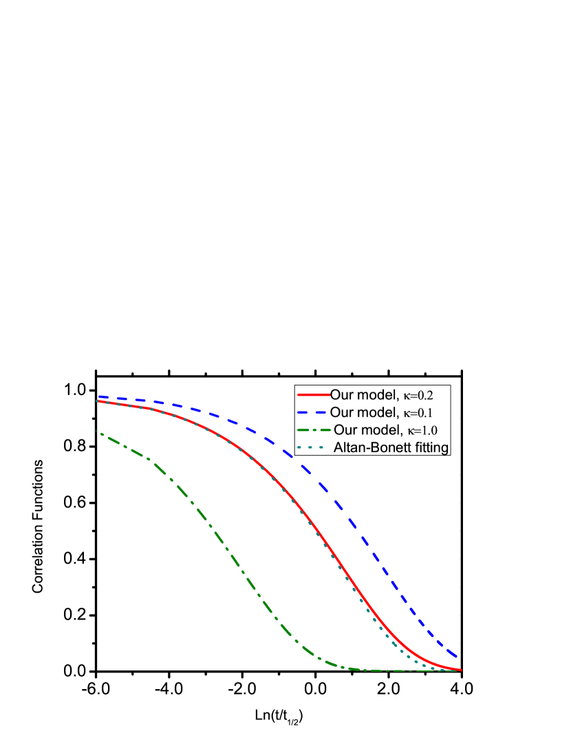
Figure 1: The autocorrelation function against time ($t/t_{1/2}$). The values of other parameters used are: $\alpha=1,L=10,k=100,\zeta=5,k_{B}T=1$.

IV Conclusions

The stochastic dynamics of DNA bubble formed due to rupture and reformation of hydrogen bonds is modeled based on a Rouse chain description of the DNA strand. Although the model is very simple it produces the experimental results of Altan-Bonett reasonably well. Unlike other well known models Fogedby and Metzler (2007); Chatterjee et al. (2007) our model goes beyond a single reaction coordinate or order parameter description by taking into account of the collective nature of the dynamics through different modes of the chain as is done in the Rouse description in the simplest possible way. The dynamics seems to be very sensitive to the relaxation times of different normal modes of the chain which is physically understandable as the “bubble dynamics” should have the contribution from all the possible normal mode of vibration of the chain. However the current model probably can not account for the bubble size distribution. We are in the process of developing a more realistic model which can account for the issue like bubble size distribution.

V acknowledgement

The author thanks K. L. Sebastian for encouragements.

References

• Watson and Crick (1953) J.Β D. Watson and F.Β H.Β C. Crick, Nature (London) 171, 737 (1953).
• Altan-Bonnet etΒ al. (2003) G.Β Altan-Bonnet, A.Β Libchaber, and O.Β Kirchevsky, Phys. Rev. Lett. 90, 138101 (2003).
• Fogedby and Metzler (2007) H.Β C. Fogedby and R.Β Metzler, Phys. Rev. Lett. 98, 070601 (2007).
• Poland and Scheraga (1966) D.Β Poland and H.Β A. Scheraga, J. Chem. Phys. 45, 1456 (1966).
• Chatterjee etΒ al. (2007) D.Β Chatterjee, S.Β Chaudhury, and B.Β J. Cherayil, J. Chem. Phys. 127, 155104 (2007).
• Doi and Edwards (1988) M.Β Doi and S.Β F. Edwards, The Theory of Polymer Dynamics (Clarendon Press. Oxford, 1988).
• Kawakatsu (2004) T.Β Kawakatsu, Statistical Physics of Polymers An Introduction (Springer, 2004).
• Kubo etΒ al. (2003) R.Β Kubo, M.Β Toda, and N.Β Hashitsume, Statistical Physics II: Nonequilibrium Statistical Mechanics (Springer Series in Solid-State Sciences) (Springer, 2003).
• Bicout (2004) D. J. Β Bicout and K. Kats, Phys. Rev. E 70, 010902(R) (2004).
• Jeon (2006) J.Β Jeon, W.Β Sung, and F. H. Ree, J. Chem. Phys. 124, 164905 (2006).
• Srivastava (2009) S. Β Srivastava and Y. Singh, Euro. Phys. Lett. 85, 38001 (2009).
• Bicout (1993) T. Β Dauxois, M.Β Peyard, and A. R. Bishop, Phys. Rev. E 47, 684 (1993).