NSPT study of the three-loop lattice gluon propagator in Landau gauge

Abstract:

By means of Numerical Stochastic Perturbation Theory (NSPT), we calculate the lattice gluon propagator up to three loops of perturbation theory in the limits of infinite volume and vanishing lattice spacing. Based on known anomalous dimensions and a parametrization of both the hypercubic symmetry group $H(4)$ and finite-size effects, we calculate the non-leading-log and non-logarithmic contributions iteratively, starting with the first-loop expression.

BI-TP 2010/36, HU-EP-10/60, LU-ITP 2010/007

1 Introduction

This talk was given as a progress report summarizing our work on the perturbative gluon propagator that has, in the meantime, published in Ref. [1]. This work is a continuation of Ref. [2] that was focused on the ghost propagator. The Monte Carlo study of both propagators (for a recent discussion see [3]), which are closely related to each other by Schwinger-Dyson equations (SDE) [4], has attracted much attention outside the lattice community by phenomenologists working in infrared QCD and hadron physics. For many reasons, the (covariant) Landau gauge propagators have been the centre of interest. The importance for the confinement problem has been discussed in Ref. [5].

Taken together, both propagators provide us with a definition and the momentum dependence of the running coupling $\alpha_{s}(q^{2})$ directly based on the ghost-gluon vertex. This has recently turned out to be an interesting frame to accurately measure $\alpha_{s}(M_{z})$ from propagators [6, 7, 8].

A simple connection between the two propagators exists in the extreme infrared, powerlike in a scaling and massive in a decoupling version. Only the latter is found on the lattice, while both solutions can be accommodated in the SDE approach. Some ideas exist today [9] about how to handle the Gribov ambiguity such that the scaling solution could eventually be reproduced on the lattice.

In a wider sense, the effect of nontrivial vacuum structure (vortices, instantons) is manifest [10, 11] also in the gluon propagator, in the intermediate momentum range around ${\cal O}(1\mathrm{~{}GeV})$ where the SDE approach suffers from truncation ambiguities and where nonperturbative lattice calculations are unrivalled. In order to understand the onset of nonperturbative effects, it is important to approach this momentum range from high momenta within higher-order perturbation theory. Some of us have started such a program a couple of years ago [12]. While ordinary diagrammatic lattice perturbation theory soon gets too involved to be pursued, Numerical Stochastic Perturbation Theory (NSPT, for a recent review see Ref. [13] and references therein), provides a powerful tool to perform high-loop computations. One has to run coupled Langevin simulations on the lattice and to perform the necessary limits: Langevin time step $\epsilon\to 0$, volume $V\to\infty$ and lattice spacing $a\to 0$.

The infinite-volume and continuum extrapolation part of the program has been satisfactorily achieved in Refs. [2, 1], such that the otherwise difficult to access non-logarithmic contributions became calculable. We refer the interested reader to these papers for more details about the technique of NSPT and the procedure to take the needed limits. The method to perform the $V\to\infty$ and $a\to 0$ limits simultaneously has been outlined for the first time in Ref. [2] for the ghost propagator and applied to the gluon propagator in Ref. [1]. There we have attempted to compare the perturbative results summed to the presently known order with the results of Monte Carlo simulations. In this short account of our work we concentrate on the method to extract all non-leading-log and non-logarithmic coefficients of the gluon dressing function from NSPT data.

2 The gluon dressing function

Recalling that the gluon propagator has to be color-diagonal and symmetric in the Lorentz indices, its tensor structure in the continuum can be written as

$$D_{\mu\nu}^{ab}(p)=\delta^{ab}\Bigg{[}\Bigg{(}\delta_{\mu\nu}-\frac{p_{\mu}p_{\nu}}{p^{2}}\Bigg{)}D(p^{2})+\frac{p_{\mu}p_{\nu}}{p^{2}}\frac{F(p^{2})}{p^{2}}\Bigg{]}\;,$$ (1)

where the transverse part $D(p^{2})$ and the longitudinal part $F(p^{2})$ have been introduced. The latter vanishes in the Landau gauge. The lattice counterpart $D_{\mu\nu}^{ab}(p(k))$  of Eq. (2.1) generally contains more terms on the r.h.s. due to the lower symmetry. The quantity under study, surviving the continuum limit, is

$$D(p(k))=\frac{1}{3}\sum_{\mu=1}^{4}D_{\mu\mu}(p(k))\;,$$ (2)

where color indices are dropped from now on to ease the notation. Eq. (2.2) obviously corresponds to the transverse propagator. In the following we use the $n^{th}$-order dressing function $J_{(n)}(p)$ defined as

$$J_{(n)}(p)=p^{2}D_{(n)}(p(k))\;.$$ (3)

3 The non-logarithmic contributions to Z

In the RI’-MOM scheme, the relation between the bare dressing function $J_{0}(p,a,\alpha_{RI^{\prime}})$ and its renormalized counterpart $J_{RI^{\prime}}(p,\mu,\alpha_{RI^{\prime}})$ is given by 

$$J_{0}(p,a,\alpha_{RI^{\prime}})\ \!=\ \!Z(a,\mu,\alpha_{RI^{\prime}})\ \!J_{RI^{\prime}}(p,\mu,\alpha_{RI^{\prime}})\;,$$ (4)

with the renormalization condition $\left.J_{RI^{\prime}}(p,\mu,\alpha_{RI^{\prime}})\right|_{p^{2}=\mu^{2}}=1$ and with $\alpha_{RI^{\prime}}=g^{2}(a\mu)/16\pi^{2}$. More in detail, the objects in Eq. (3.1) can be perturbatively expanded as

$$Z(a,\mu,\alpha_{RI^{\prime}}) = 1+\sum_{n>0}\alpha_{RI^{\prime}}^{n}\sum_{j=0}^{n}z_{\ \!n,j}^{RI^{\prime}}\ \!\log^{j}(a\mu)\ ,$$ (5)

$$J_{0}(p,a,\alpha_{RI^{\prime}}) = 1+\sum_{n>0}\alpha_{RI^{\prime}}^{n}\sum_{j=0}^{n}z_{\ \!n,j}^{RI^{\prime}}\ \!\bigg{(}\frac{1}{2}\log(ap)^{2}\bigg{)}^{\!\!j}\ ,$$ (6)

$$J_{RI^{\prime}}(p,\mu,\alpha_{RI^{\prime}}) = 1+\sum_{n>0}\alpha_{RI^{\prime}}^{n}\sum_{j=0}^{n}z_{\ \!n,j}^{RI^{\prime}}\ \!\bigg{(}\frac{1}{2}\log(p\mu^{-1})^{2}\bigg{)}^{\!\!j}\;.$$ (7)

By plugging the perturbative expansions above into Eq. (3.1) and by converting the renormalized coupling into the bare one, $\alpha_{0}=N_{c}/(8\pi^{2}\beta)$, the bare dressing function can be written as

$$J_{0}(p,a,\beta)=1+\sum_{n>0}\frac{1}{\beta^{n}}\sum_{j=0}^{n}J_{\ \!n,j}\ \!\log^{j}(ap)^{2}\;,$$ (8)

where the coefficients $J_{\ \!n,j}$ are related to the $z_{\ \!n,j}^{RI^{\prime}}$’s in Eq. (3.2). As far as the logarithmic contributions are concerned, their coefficients depend on the anomalous dimension of the gluon field and the $\beta-$function (see [14]). The purpose of this work is to compute the $J_{\ \!n,0}$’s which are related to the $z_{n,0}^{RI^{\prime}}$’s by

$$J_{1,0} = 0.03799544\ \!z_{1,0}^{RI^{\prime}}\ ,$$ (9)

$$J_{2,0} = 0.10673710\ \!z_{1,0}^{RI^{\prime}}+0.00144365\ \!z_{2,0}^{RI^{\prime}}\ ,$$ (10)

$$J_{3,0} = 0.375990\ \!z_{1,0}^{RI^{\prime}}+0.00811105\ \!z_{2,0}^{RI^{\prime}}+0.0000548523\ \!z_{3,0}^{RI^{\prime}}\;.$$ (11)

4 The fitting procedure

We can isolate the $n^{th}-$loop contribution in Eq. (3.5) (without power of $\beta^{-n}$) and write

$$J_{(n)}(p,a)=J_{n,0}(ap)+\sum_{j=1}^{n}\ \!J_{n,j}\ \!\log^{j}(ap)^{2}\;,$$ (12)

where, by recalling the existence of irrelevant lattice artifacts, $J_{n,0}(ap)$ can be decomposed as

$$J_{n,0}(ap)=J_{n,0}+c_{n,1}(ap)^{2}+c_{n,2}\frac{(ap)^{4}}{(ap)^{2}}+c_{n,3}(ap)^{4}+\ldots\ \ \ \ \ \ \ [(ap)^{m}\equiv\sum_{\mu}(ap_{\mu})^{m}]\;,$$ (13)

where $J_{n,0}$ is the $n^{th}-$loop constant we want to compute. Taking into account also finite-size effects, $J_{n,0}(ap)$ has to be replaced by $J_{n,0}(ap,pL)$ with

$$J_{n,0}(ap,pL) = J_{n,0}(ap)+[J_{n,0}(ap,pL)-J_{n,0}(ap)]\equiv J_{n,0}(ap)+\delta J_{n,0}(ap,pL)=$$ (14)

$$= J_{n,0}(ap)+\delta J_{n,0}(0,pL)\equiv J_{n,0}(ap)+\delta J_{n,0}(pL)\ ,$$

where, in the last two steps, $ap$ corrections on $pL$ effects are assumed to be corrections on corrections and have been neglected. Furthermore we assume that the point $p_{\max}$ corresponding to the largest $(ap)^{2}$ on the largest lattice size $L_{\max}$ is such that $\delta J_{n,0}(p_{\max}L_{\max})=0$.

When treating $pL$ contributions, it is useful to notice that, since $p_{\mu}L=p_{\mu}aN=2\pi k_{\mu}$, any given 4-tuple of integers $(k_{1},k_{2},k_{3},k_{4})$ has the same finite-size corrections to $J_{n,0}(ap)$ on different lattice sizes. Therefore, the steps in data-analysis at any loop order $n$ can be summarized as follows:

• a suitable window $[(ap)^{2}_{\min},(ap)^{2}_{\max}]$ is identified where a sufficient number of data points is available on different lattice sizes;

• the logarithmic contributions are subtracted from the bare dressing function in order to get $J_{n,0}(ap,pL)$;

• $J_{n,0}(ap,pL)$ is fitted according to the procedure sketched above: from Eq. (4.2) we compute the desired $J_{n,0}$.

Obviously, only results stemming from stable fits have to be taken into account.

5 Results

Figs. 1, 3 and 5 show an example of the fitting procedure outlined above:

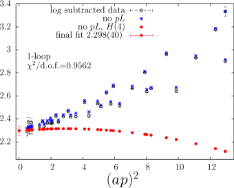
Figure 1: 1-loop data vs. $(ap)^{2}$: the different sets of points stem from the various steps of the analysis (see section 4).

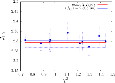
Figure 2: $J_{1,0}$ results vs. $\chi^{2}$: the dotted blue line is the average of the 10 blue points, the continuous red one is the analytical result.

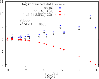
Figure 3: Same as in Fig. 1 for 2-loop data.

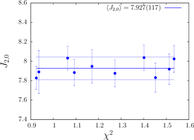
Figure 4: $J_{2,0}$ results vs. $\chi^{2}$: see caption of Fig. 2.

the black dots stand for log-subtracted data, blue stars for data after finite-size effects have been removed while red spots for data after further removal of hypercubic effects.

Loop order n	1	2	3
$J_{n,0}$	2.30(3)	7.92(12)	31.7(5)

Table 1: Results for the constant contributions to $Z$ up to the third loop. Compare the 1-loop analytical result $J_{1,0}=2.29368$.

In general, there could be various fitting functions that fulfill the stability requirement mentioned at the end of section 4: the results we quote come from averaging the values obtained from the fits with the 10 lowest $\chi^{2}$ at every perturbative order: Figs. 2, 4 and 6 contain these values and their average with their errorbars. The final outcome of the analysis sketched in the above is contained in Table 1.

Resumming the perturbative series for $J_{0}(a,p,\beta)$ up to the third loop, we get

$$J^{\rm 3-loop}(p,a,\beta) = 1+\frac{1}{\beta}\,\Bigl{(}-0.24697\,\log(ap)^{2}+2.29368\Bigr{)}+$$

$$+ \frac{1}{\beta^{2}}\,\Bigl{(}0.08211\,\left(\log(ap)^{2}\right)^{2}-1.48445\log(ap)^{2}+7.93(12)\Bigr{)}+$$

$$+ \frac{1}{\beta^{3}}\,\Bigl{(}-0.02964\,\left(\log(ap)^{2}\right)^{3}+0.81689\,\left(\log(ap)^{2}\right)^{2}+$$

$$- 8.13(3)\,\log(ap)^{2}+31.7(5)\Bigr{)}\;,$$

which can then be converted to the RI’-MOM scheme by using the formulae of section 3.

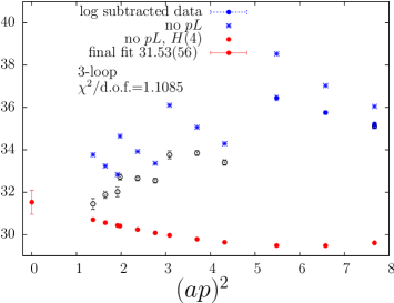
Figure 5: Same as in Fig. 1 for 3-loop data.

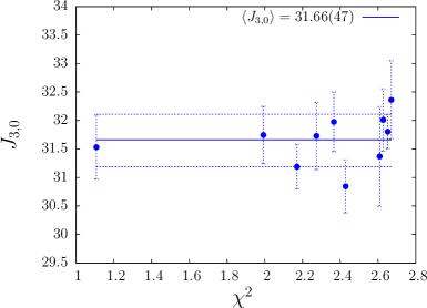
Figure 6: $J_{3,0}$ results vs. $\chi^{2}$: see caption of Fig. 2.

6 Conclusion

In this work we presented an algorithm to compute the non-logarithmic parts of infrared divergent quantities in NSPT in the infinite-volume limit using the example of the gluon propagator. The one-loop result coincides with the well-known result from the diagrammatic approach [15]. The corresponding two- and three-loop finite constants have been computed for the first time.

We can use the dressing function obtained with NSPT at finite lattice sizes to investigate the perturbative background of the corresponding Monte-Carlo calculated propagators. This has been done in some detail in [1].

References

- [1] F. Di Renzo, E.-M. Ilgenfritz, H. Perlt, A. Schiller and C. Torrero, Two-point functions of quenched lattice QCD in Numerical Stochastic Perturbation Theory. (II) The gluon propagator in Landau gauge, Nucl. Phys. B 842 (2011) 122 [hep-lat/1008.2617].
- [2] F. Di Renzo, E.-M. Ilgenfritz, H. Perlt, A. Schiller and C. Torrero, Two-point functions of quenched lattice QCD in Numerical Stochastic Perturbation Theory. (I) The ghost propagator in Landau gauge, Nucl. Phys. B 831 (2010) 262 [hep-lat/0912.4152].
- [3] I. L. Bogolubsky, E.-M. Ilgenfritz, M. Müller-Preussker, and A. Sternbeck, Lattice gluodynamics computation of Landau gauge Green’s functions in the deep infrared, Phys. Lett. B 676 (2009) 69 [hep-lat/0901.0736].
- [4] R. Alkofer and L. von Smekal, The infrared behavior of QCD Green’s functions: Confinement, dynamical symmetry breaking, and hadrons as relativistic bound states, Phys. Rept. 353 (2001) 281 [hep-ph/0007355].
- [5] R. Alkofer, C. S. Fischer, M. Q. Huber, F. J. Llanes-Estrada and K. Schwenzer, Confinement and Green functions in Landau-gauge QCD, PoS CONFINEMENT8 (2008) 019 [hep-ph/0812.2896].
- [6] A. Sternbeck et al., Running alpha(s) from Landau-gauge gluon and ghost correlations, PoS LAT2007 (2007) 256 [hep-lat/0710.2965].
- [7] L. von Smekal, K. Maltman and A. Sternbeck, The strong coupling and its running to four loops in a minimal MOM scheme, Phys. Lett B 681 (2009) 336 [hep-ph/09031696].
- [8] A. Sternbeck, E.-M. Ilgenfritz, K. Maltman, M. Müller-Preussker, L. von Smekal and A.G. Williams, QCD Lambda parameter from Landau-gauge gluon and ghost correlations, PoS LAT2009 (2009) 210 [hep-lat/1003.1585].
- [9] A. Maas, Constructing non-perturbative gauges using correlation functions, Phys. Lett B 689 (2010) 107 [hep-lat/0907.5185].
- [10] K. Langfeld, H. Reinhardt and J. Gattnar, Gluon propagators and quark confinement, Nucl. Phys. B 621 (2002) 131 [hep-ph/0107141].
- [11] Ph. Boucaud et al., Evidences for instantons effects in Landau lattice Green functions, Phys. Rev. D 70 (2004) 114503 [hep-ph/0312332].
- [12] E.-M. Ilgenfritz, H. Perlt, and A. Schiller, The lattice gluon propagator in stochastic perturbation theory, PoS LAT2007 (2007) 251 [hep-lat/0710.0560].
- [13] F. Di Renzo and L. Scorzato, Numerical Stochastic Perturbation Theory for full QCD, JHEP 0410 (2004) 073 [hep-lat/0410010].
- [14] J. Gracey, Three loop anomalous dimension of non-singlet quark currents in the RI’ scheme, Nucl. Phys. B 662 (2003) 247 [hep-ph/0403113].
- [15] H. Kawai, R. Nakayama and K. Seo, Comparison Of The Lattice Lambda Parameter With The Continuum Lambda Parameter In Massless QCD, Nucl. Phys. B 189 (1981) 40.