RESCEU-23/10

COSMOLOGICAL CONSTANT FROM DECOHERENCE
Claus Kiefer and Friedemann Queisser
Institut für Theoretische Physik, Universität zu Köln,

Zülpicher Strasse 77, 50937 Köln, Germany.
Alexei A. Starobinsky
Landau Institute for Theoretical Physics, Moscow 119334, Russia and

RESCEU, Graduate School of Science, The University of Tokyo, Tokyo 113-0033, Japan

Abstract

We address the issue why a cosmological constant (dark energy) possesses a small positive value instead of being zero. Motivated by the cosmic landscape picture, we mimic the dark energy by a scalar field with potential wells and show that other degrees of freedom interacting with it can localize this field by decoherence in one of the wells. Dark energy can then acquire a small positive value. We also show that the additional degrees of freedom enhance the tunneling rate between the wells. The consideration is performed in detail for the case of two wells and then extended to a large number of wells.

1 Introduction

Observations indicate that our Universe is currently accelerating [1]. The simplest explanation of this fact in terms of the Einstein equations of gravity is the existence of a non-zero Einstein cosmological constant $\Lambda$. However, a more general dynamical entity dubbed “dark energy” (DE), whose effective energy–momentum tensor is close to that of $\Lambda$, is also a serious possibility [2, 3, 4, 5, 6, 7]. Present measurements of the effective DE equation of state $w_{\rm DE}:=p_{\rm DE}/\rho_{\rm DE}$ are inconclusive about its nature and are compatible with DE being given exactly by $\Lambda$, that is, with $w_{\rm DE}\equiv-1$ [1].

The microscopic origin of DE is presently unknown and can perhaps only be explained after a full quantum theory of gravity is available [8]. There are actually two aspects connected with DE. First, it is unclear why the effective energy density of DE (or $\Lambda$ itself) is much smaller than one would expect from elementary particle physics on dimensional grounds. Second, it is unclear why it is not exactly zero but has a small positive value. The first question might only be answered on the basis of a full quantum theory of all quantum fields including gravity. But it is possible that the second question can be addressed on the basis of known physics.

A first step in the understanding of the second question was made by Yokoyama [9]. He modelled DE by a scalar field $\phi$ with a potential $V(\phi)$ that is characterized by a double well. This choice can be motivated by recent ideas in string theory, where a “landscape” of many (perhaps as many as $10^{500}$ or more) local minima of a complicated potential is discussed, see, for example, [10, 11] and the references therein. Yokoyama assumed that, perhaps due to some unknown symmetry, the exact ground state of the Universe is characterized by a vanishing vacuum energy, that is, a vanishing cosmological constant and that the observed small deviation from zero could arise from the fact that the Universe is not in its ground state.

But how can this happen? The ground state for a double-well potential is extended (delocalized) over both minima. In contrast to this, a state localized in one of the minima is a superposition of the eigenstates; in the simplest case, it is a superposition of the ground and the first excited state. The effective energy of such localized states is greater than the ground-state energy and would therefore be positive if the ground-state energy were zero. If the wall between the wells is not too small, the values for this positive-energy states are tiny because they differ from the ground-state energy only by a small tunneling factor proportional to $\exp(-S_{0})$, where $S_{0}$ is the instanton action. The reason for the observed small positive cosmological constant could thus lie in the fact that the dark energy in the Universe is in a localized state that is concentrated near one of the minima of the potential.

As long as the universe stays in such a localized state, the effective DE equation of state will be $w_{\rm DE}\approx-1$. There exists, however, a certain probability that the Universe can evolve into the ground state, which is a superposition of the localized states, or tunnel into another localized state. The question then arises how large the time scale and the tunneling rate would be. Obviously, these scales should obey all known observational constraints presented in [1].

In our paper we shall elaborate on this idea in two respects. First, it has to be justified why a DE field is not found in its ground state in the first place, but in a localized state. This is reminiscent of an analogous situation in quantum mechanics where chiral molecules are typically found in left-handed or right-handed isomeric forms and not in a superposition of the two (as e.g. the ground state would be). Historically, this was called “Hund’s paradox” [12]. Its solution is based on the central concept of decoherence [12, 13] and was recently presented for a specific case in quantitative detail in [14]. Decoherence is the unavoidable and irreversible emergence of classical properties with its environment; “environment” stands here for any irrelevant degrees of freedom that interact with the quantum system and thereby become entangled with it. In the case of the chiral molecules these can be photons or air molecules scattering off these molecules. Decoherence will also play a central role in our analysis, in order to explain why the DE field is not in its delocalized ground state, but in a localized state with higher energy.

Our second elaboration is a direct consequence of the first one. If additional “decohering” degrees of freedom are present, they will have an effect on the tunneling rate from one well to the other. We shall thus discuss both the pure tunneling rate of the isolated system as well as its modification by the environment. In view of the experience from quantum mechanical models [15], one would expect that these degrees of freedom will in general reduce this rate, so that tunneling will become less likely. In contrast to this expectation, however, we shall find that this tunneling rate is here increased rather than decreased, by a field-theoretic mechanism similar to the Casimir effect. The localization by the environment together with the magnitude of the tunneling rate could then provide the explanation of why we observe a small positive value for dark energy.

We note that our approach is completely different from the one used in the paper [16] (which appeared when our paper was prepared for publication), where entanglement between different cosmological epochs, not different vacua, is proposed as a source of $\Lambda$.

Our considerations should also be relevant for the inflationary stage in the early Universe, which was dominated by a primordial DE whose properties were close to an effective (though metastable) cosmological constant, too. However, we do not attempt here an application in this direction.

Our paper is organized as follows. In Sec. 2.1 we present our model: DE is modelled by a scalar field (quintessence), and it interacts with an environmental massless scalar field that may arise from metric perturbations. In Sec. 2.2 the process of decoherence is discussed in detail for both sub- and super-Hubble modes of the environment. It is found that these modes localize the DE field in one well, the super-Hubble modes even more efficiently than the sub-Hubble modes. In Sec. 3 we calculate the tunneling rate for a Minkowski background as well as an expanding Universe. We find that the presence of an environmental field enhances the original tunneling rate. In order to approach more closely the ideas of a cosmic landscape, we extend our discussion in Sec. 4 to the presence of many vacua. A brief Appendix summarizes some material about the $\zeta$-function renormalization needed in Sec. 3.

Our main results have already been briefly announced in [17].

2 Small positive dark energy from decoherence

2.1 The model

We present here our model in which a scalar field $\phi$ mimicking DE (called the “system” in the following) is coupled to other degrees of freedom called “environment”. As in the Yokoyama paper [9], $\phi$ is assumed to possess a potential with two quasi-localized minima. As for the environment, we choose another scalar field called $\sigma$ which couples to $\phi$. The details of the interaction are of secondary importance; it only has to be able to generate a sufficient entanglement between system and environment [12].

Both system and environment are supposed to evolve in a flat Friedmann-Robertson-Walker (FRW) background with the line element

$$ds^{2}=g^{\rm B}_{\mu\nu}dx^{\mu}dx^{\nu}=dt^{2}-a^{2}(t)(dx^{2}+dy^{2}+dz^{2})$$ (1)

($\hbar=c=1$ is set throughout the paper). We assume here for later convenience that the scale factor, $a$, has the dimension of a length, while $x$, $y$, and $z$ are dimensionless. The total action of system and environment then reads

$$S=\int d^{4}x\sqrt{-g^{\mathrm{B}}}\left(\mathcal{L}_{\rm sys}+\mathcal{L}_{\rm env}+\mathcal{L}_{\rm int}\right)\,,$$ (2)

where $g^{\mathrm{B}}$ is the determinant of the metric $g^{\rm B}_{\mu\nu}$, and $\mathcal{L}_{\rm sys}$, $\mathcal{L}_{\rm env}$, and $\mathcal{L}_{\rm int}$ denote the Lagrangian of the system, environment, and interaction, respectively. The spatially homogeneous scalar field describing the vacuum energy reads

$$\mathcal{L}_{\rm sys}:=\frac{1}{2}\dot{\phi}^{2}-V(\phi)\,,$$ (3)

while the Lagrangian of the environment, $\mathcal{L}_{\rm env}$, describes a massless scalar field $\sigma$,

$$\mathcal{L}_{{\rm env},\sigma}:=\frac{1}{2}g^{\rm B\mu\nu}\partial_{\mu}\sigma\partial_{\nu}\sigma\,.$$ (4)

The interaction between system and environment must be able to discriminate between different values of the scalar field $\phi$. In quantum mechanical applications one often chooses a bilinear interaction, see for instance the Caldeira–Leggett model [15] or the spin–boson model described, for example, in Section 5.3 of [13]. Since, however, our field $\phi$ is spatially homogeneous, a bilinear term of the form $\int d^{3}x\ \sigma(\mathbf{x},t)\phi(t)$ would give no interesting dynamics, since only a single Fourier component of the scalar field $\sigma$, the one with vanishing momenta, would interact with the system field. We therefore introduce the tri-linear interaction

$$\mathcal{L}_{{\rm int},\sigma}:=-g_{\rm s}\sigma^{2}\phi\,$$ (5)

for the coupling with the scalar-field environment. Here, the coupling constant $g_{\rm s}$ has to be chosen such that the product $g_{\rm s}\phi$ is positive. This guarantees that the corresponding Hamiltonian is bounded from below and that the dynamics is thus stable. Since both $\sigma^{2}$ and $\phi^{2}$ have physical dimension mass ($M$) over length ($L$), the dimension of $g_{\rm s}$ is $(ML^{3})^{-1/2}$, which in the natural units used here is equal to $M$.

What could be the origin of such a coupling? It can arise, for example, from the expansion of the metric determinant $\sqrt{-g}$ into the scalar and tensor modes. Let us consider therefore the FRW line element with scalar and tensor perturbations (see e.g. [18]),

$$ds^{2}=(1+2\psi_{1})dt^{2}-a^{2}\left[(1-2\psi_{2})\delta_{ij}+h_{ij}\right]dx^{i}dx^{j}\,,$$ (6)

where $\psi_{1/2}$ are scalar perturbations and $h_{ij}$ are tensor modes. In the transverse and traceless gauge, there are only two independent tensor modes, $h_{23}=h_{32}$ and $h_{22}=-h_{33}$. If there is a linear term in the potential of the system field $\phi$, we get from the expansion of the determinant a term of the form

$$\int d^{3}x\sqrt{-g}\phi\approx$$ (7)

$$\int d^{3}x\sqrt{-g^{B}}\left(1+\psi_{1}-3\psi_{2}-2\psi_{1}^{2}+\frac{3}{2}(\psi_{1}-\psi_{2})^{2}-\frac{1}{2}h_{22}^{2}-\frac{1}{2}h_{23}^{2}\right)\phi\,.$$

Discarding the terms linear in $\psi_{1}$ and $\psi_{2}$ for the reason mentioned above, we are left with tri-linear interactions of the form (5); the role of our field $\sigma$ could thus be played by $\psi_{1}$, $\psi_{2}$, $h_{22}$, or $h_{23}$. Such interactions can thus arise both from the scalar and the tensor perturbations of the metric itself, although it is conceivable that $\sigma$ is any other field that occurs in a fundamental theory.

We shall now address the Hamiltonian that will be used in the quantum theory. It can be derived from (2)–(5) and in the momentum representation reads

$$H_{\phi,\sigma} = \int dp^{3}\Bigg{(}\frac{1}{2a^{3}}\tilde{\Pi}(\mathbf{p})\tilde{\Pi}(-\mathbf{p})+\frac{a}{2}p^{2}\tilde{\sigma}(\mathbf{p})\tilde{\sigma}(-\mathbf{p})$$

$$+g_{\rm s}a^{3}\phi\tilde{\sigma}(\mathbf{p})\tilde{\sigma}(-\mathbf{p})\Bigg{)}+H_{\phi}\,,$$

where

$$\sigma(\mathbf{x}) = \frac{1}{(2\pi)^{3/2}}\int d^{3}p\ \tilde{\sigma}_{ab}(\mathbf{p})e^{i\mathbf{x}\mathbf{p}}\,,$$ (9)

$$\Pi(\mathbf{x}) = \frac{1}{(2\pi)^{3/2}}\int d^{3}p\ \tilde{\Pi}(\mathbf{p})e^{i\mathbf{x}\mathbf{p}}\,,$$ (10)

and $H_{\phi}$ denotes the pure $\phi$-Hamiltonian (see (11) below). Note that $\mathbf{p}$ is dimensionless because $\mathbf{x}$ is dimensionless.

In the following, we shall simplify the part of the Hamiltonian describing the system. We shall assume that the dynamics of the system is dominated by the two lowest energy eigenvalues of the double-well potential, that is, we assume that their difference is much smaller than the energy gaps within a single well. It is then possible to reduce the system to an effective two-state system,

$$H_{\phi}=\begin{pmatrix}E_{+}&\Delta\\ \Delta&E_{-}\end{pmatrix}\,,$$ (11)

where $E_{+}$ and $E_{-}$ are the energy levels of the localized minima, and $\Delta$ is the tunneling matrix element.

The reduction of the system to an effective two-state system leads to the interaction

$$H_{{\rm int},\sigma}=g_{\rm s}a^{3}(t)\begin{pmatrix}\phi_{+}&0\\ 0&\phi_{-}\end{pmatrix}\int d^{3}p\ \sigma(\mathbf{p})\sigma(-\mathbf{p})\,,$$ (12)

where the environment can only discriminate between the two different minima of the potential, $\phi_{+}$ and $\phi_{-}$.

All together, our model resembles a spin–boson model [13], although the coupling in the standard situation is taken to be linear in the environmental fields. It is well known that situations with a double-well potential can often be described by an effective two-state system [12, 13]. In this context the Hamiltonian (11) would be written in the form

$$H_{\phi}=\sigma_{x}\Delta+\frac{1}{2}(\delta E)\sigma_{z}+\frac{1}{2}(E_{+}+E_{-}){\mathbb{I}}\ ,$$

where $\sigma_{x}$ and $\sigma_{z}$ are Pauli matrices, and $\delta E:=E_{+}-E_{-}$. Spin–boson models describe the interaction of a central system with its environment in the case when the system is effectively acting as a two-level system.

2.2 The reduced density matrix

With this simplification at hand, it is possible to calculate the reduced density matrix of the two-state system. We assume that the initial state is a product of a system and an environmental state, $|\Psi\rangle_{\mathrm{sys}}\otimes|\Psi\rangle_{\mathrm{env}}$. The time evolution will then generate an entanglement between them. This evolution is governed by the functional Schrödinger equation

$$i|\dot{\Psi}\rangle=H_{\mathrm{\phi,\sigma}}|\Psi\rangle\ .$$ (13)

In this section, we shall neglect tunneling, that is, we set $\Delta=0$ in (11); this enables us to solve the Schrödinger equation exactly. We assume that the state of system and environment is of Gaussian form (see e.g. [19, 20, 21]) and make the ansatz

$$|\Psi\rangle=\begin{pmatrix}\alpha N_{+}(t)\exp\left(-\frac{1}{2}\int d^{3}p\ \sigma(\mathbf{p})\Omega_{+}(\phi,p,t)\sigma(-\mathbf{p})-iE_{+}t\right)\\ {}\\ \beta N_{-}(t)\exp\left(-\frac{1}{2}\int d^{3}p\ \sigma(\mathbf{p})\Omega_{-}(\phi,p,t)\sigma(-\mathbf{p})-iE_{-}t\right)\end{pmatrix}\,,$$ (14)

where $\Omega_{+/-}(p,t)$ and $N_{+/-}(t)$ are time-dependent functions to be determined from the Schrödinger equation, and $\alpha$ and $\beta$ are constants with $|\alpha|^{2}+|\beta|^{2}=1$. With the above ansatz one obtains the following Riccati-type equations, cf. [20],

$$-i\dot{\Omega}_{+/-}(p,t)=-\frac{(\Omega_{+/-}(p,t))^{2}}{a^{3}}+p^{2}a+g_{\rm s}a^{3}\phi_{+/-}$$ (15)

and

$$\frac{1}{2a^{3}}\mathrm{Tr}\,\Omega_{+/-}(p,t)=i\frac{\dot{N}_{+/-}}{N_{+/-}}\,.$$ (16)

Eq. (15) can be transformed by the ansatz

$$\Omega_{+/-}(p,t)=:-ia^{3}\frac{\dot{u}_{+/-}(p)}{u_{+/-}(p)}$$ (17)

into a linear equation for ${u}_{+/-}$. Switching to conformal time, which is defined by $a\,d\eta=dt$, and denoting derivatives with respect to $\eta$ by a prime, we obtain

$$(p^{2}+\gamma a^{2})u_{+/-}(p,\eta)+\frac{2a^{\prime}}{a}{u^{\prime}}_{+/-}(p,\eta)+{u^{\prime\prime}}_{+/-}(p,\eta)=0\,,$$ (18)

where we have introduced the quantity

$$\gamma:=2g_{\rm s}\phi_{+/-}\ ,$$ (19)

which has dimension $L^{-2}\equiv M^{2}$ and obeys $\gamma>0$. (We have skipped the indices $+/-$ in $\gamma$ for simplicity.) We assume that the coupling between system and environment is small, that is, $\gamma<H^{2}$. The total density matrix for system and environment is given by the pure state

$$\rho(t)=|\Psi\rangle\langle\Psi|\ ,$$ (20)

from which the reduced density matrix is obtained by integrating out the environmental scalar field,

$$\rho(t)_{\mathrm{sys}}:=\mathrm{Tr}_{\mathrm{env}}|\Psi\rangle\langle\Psi|\,.$$ (21)

In position representation, this reads

$$\rho_{ij}=\int{\mathcal{D}}\sigma\ \Psi_{i}^{*}[\sigma]\Psi_{j}[\sigma]\ ,$$ (22)

where $i,j$ run over the values $+$ and $-$, and $\Psi\equiv(\psi_{+}\ \psi_{-})^{\rm T}$. Since by setting $\Delta=0$ we have neglected dissipation, the diagonal elements of the reduced density matrix remain unchanged, that is, one has

$$\rho_{++}(t) = |\alpha|^{2}|N_{+}(t)|^{2}\int\mathcal{D}\sigma\exp\left[-\int d^{3}p\ \sigma(\mathbf{p})\Re\Omega_{+}(t)\sigma(-\mathbf{p})\right]$$ (23)

$$= |\alpha|^{2}=\rho_{++}(0)$$

and analogously $\rho_{--}(t)=\rho_{--}(0)$. The probabilities of finding the system in state $+$ or $-$ are thus unchanged by the environment; this corresponds to a quantum-nondemolition (or ideal) measurement [12, 13].

The non-diagonal elements can be calculated as follows:

$$\rho_{+-}(t) = \rho_{-+}^{*}(t)=\alpha\beta^{*}N_{+}\left(N_{-}\right)^{*}\times$$

$$\int D\sigma\exp\left(-\frac{1}{2}\int d^{3}p\ \sigma(\mathbf{p})\left(\Omega_{+}+\left(\Omega_{-}\right)^{*}\right)\sigma(-\mathbf{p})-i(E_{+}-E_{-})t\right)$$ (24)

$$= \alpha\beta^{*}\frac{\det^{1/4}(\Re\Omega_{+})\det^{1/4}(\Re\Omega_{-})}{\det^{1/2}\left(\left(\Omega_{+}+\left(\Omega_{-}\right)^{*}\right)/2\right)}\times$$

$$\times\exp\left(-i\int^{t}dt^{\prime}\frac{1}{2a^{3}}\mathrm{Tr}(\Re\Omega_{+}-\Re\Omega_{-})-i(E_{+}-E_{-})t\right)\,.$$

From (18) we can see that the functions $\Omega_{+/-}$ depend on the small parameter $a^{2}\gamma/p^{2}$ for sub-Hubble modes and on $\gamma/H^{2}$ for super-Hubble modes, see below for an explanation of these terms. Expanding $\Omega_{+/-}$ up to second order in $\gamma$ yields

$$\Omega_{+/-}(\gamma) \approx \Omega_{+/-}\Bigg{|}_{\gamma=0}+\frac{d}{d\gamma}\Omega_{+/-}\Bigg{|}_{\gamma=0}\gamma+\frac{1}{2}\frac{d^{2}}{d\gamma^{2}}\Omega_{+/-}\Bigg{|}_{\gamma=0}\gamma^{2}$$ (25)

$$=: \Omega+\Omega_{\gamma}\gamma+\frac{1}{2}\Omega_{\gamma\gamma}\gamma^{2}\ ,$$

where derivatives with respect to $\gamma$ are denoted by indices. (Strictly speaking, the expansion is with respect to the dimensionless combinations $a^{2}\gamma/p^{2}$ or $\gamma/H^{2}$.)

The approximate expression for the non-diagonal elements then reads

$$\rho_{+-}(t)=\rho_{+-}(0)\exp\left(-\frac{g_{\rm s}^{2}(\phi_{+}-\phi_{-})^{2}}{4}\mathrm{Tr}\left(\frac{(\Re\Omega_{\gamma})^{2}+(\Im\Omega_{\gamma})^{2}}{(\Re\Omega)^{2}}\right)-i\varphi_{+-}\right)$$ (26)

with $\rho_{+-}(0)=\alpha\beta^{*}$ and

$$\varphi_{+-} = \mathrm{Tr}\left(\frac{\Im\Omega_{\gamma}}{\Re\Omega}\frac{g_{\rm s}(\phi_{+}-\phi_{-})}{2}+\left(\frac{\Im\Omega_{\gamma\gamma}}{\Re\Omega^{S}}-\frac{\Im\Omega_{\gamma}\Re\Omega_{\gamma}}{(\Re\Omega)^{2}}\right)\frac{g_{\rm s}^{2}(\phi_{+}^{2}-\phi_{-}^{2})}{2}\right)$$ (27)

$$+ \int^{t}d\tilde{t}\ \frac{1}{2a^{3}}\mathrm{Tr}(\Re\Omega_{+}-\Re\Omega_{-})+(E_{+}-E_{-})\tilde{t}\,.$$

In the following, we want to discuss the explicit form of the decoherence factor. To begin with, we consider the impact of the sub-Hubble modes on the system, that is, the impact of modes whose wavelength $\lambda=2\pi a/p$ is smaller than the Hubble scale $H^{-1}$. Using a WKB-approximation, which is adequate for $p^{2}\gg a^{\prime\prime}/a$, the solutions to the differential equation (18) read

$$u_{+/-}(p,\eta)=\frac{A}{a}\exp\left(i\int^{\eta}d\tilde{\eta}\ \omega_{+/-}(\tilde{\eta})\right)\ ,$$ (28)

where

$$\omega_{+/-}(\eta):=\left(p^{2}+\gamma a^{2}-\frac{a^{\prime\prime}}{a}\right)^{1/2}\,.$$ (29)

We have chosen an adiabatic vacuum in the infinite past for each Fourier mode ${\bf p}$. This choice is possible because the interaction vanishes for $a\rightarrow 0$ when the modes are far inside the horizon. In the case of a massive scalar field ($g_{s}\phi_{+/-}>0$) in the exact de Sitter background, it leads to the Bunch–Davies vacuum for the whole field $\sigma$, see e.g. [22]. The trace of the real part of the exponent in (26) is

$$\mathrm{Tr}\left(\frac{(\Re\Omega_{\gamma})^{2}+(\Im\Omega_{\gamma})^{2}}{(\Re\Omega)^{2}}\right)=\frac{\pi a^{4}V}{(2\pi)^{3}}\int_{p_{\mathrm{min}}}^{\infty}dp\ \frac{p^{2}}{\left(p^{2}-\frac{a^{\prime\prime}}{a}\right)^{2}}$$ (30)

$$= \frac{a^{4}V}{16\pi^{2}}\left(\frac{p_{\mathrm{min}}}{p_{\mathrm{min}}^{2}-\frac{a^{\prime\prime}}{a}}+\frac{1}{2}\sqrt{\frac{a}{a^{\prime\prime}}}\ln\left(\frac{p_{\mathrm{min}}+\sqrt{\frac{a^{\prime\prime}}{a}}}{p_{\mathrm{min}}-\sqrt{\frac{a^{\prime\prime}}{a}}}\right)\right)\,,$$

where $V$ denotes the dimensionless coordinate volume which must be fixed by an appropriate infrared cutoff. The WKB-approximation holds for modes far inside the horizon, $p_{\mathrm{min}}>\sqrt{a^{\prime\prime}/a}$; in the case of a constant Hubble rate, we have $p_{\mathrm{min}}>\sqrt{2}Ha$.

To discuss the explicit form of the decoherence rate for super-Hubble modes, that is, for modes with wavelengths greater than the Hubble scale, we shall restrict ourselves to the expanding de Sitter case where $H=\mathrm{constant}.$ In this case, it is not possible to find WKB solutions valid for all times including $t\to\infty$ ($\eta\to 0)$, because the time evolution for super-Hubble modes is highly nonadiabatic. The solution of Eq. (18) that has the correct WKB behavior for $\eta\to-\infty$ is then given by

$$u_{+/-}(p,\eta)=\frac{H\sqrt{\pi}}{2}\left(\frac{\eta}{p}\right)^{3/2}\mathcal{H}^{(1)}_{\sqrt{9/4-\gamma/H^{2}}}(p\eta)\ ,$$ (31)

where $\mathcal{H}^{(1)}$ denotes a Hankel function. (Recall that $\gamma<H^{2}$.) In the massless case $g_{\rm s}=0$, this expression reduces to the textbook free field solution for the adiabatic (WKB) initial vacuum state at $\eta\to-\infty$:

$$u_{g_{\rm s}=0}(p,\eta)=-\frac{H\eta}{\sqrt{2}p^{2}}\left(1+\frac{i}{p\eta}\right)e^{ip\eta}\,.$$ (32)

Note that due to the absence of WKB solutions for $t\to\infty$ ($\eta\to 0$), there exists an ambiguity in the definition of a particle for super-Hubble modes for sufficiently small masses $m^{2}=\gamma^{2}\leq 9H^{2}/4$. In addition, these modes are strongly squeezed. In particular, in the massless case $g_{s}=0$ we have

$$\sinh^{2}r_{p}=\frac{a^{2}H^{2}}{4p^{2}}\,,$$ (33)

where $r_{p}$ is the squeezing parameter of the mode, see e.g. [23, 24]. On the other hand, in the exact de Sitter case it is possible, in principle, to consider the whole solution (32) as the second-order corrected WKB solution that would imply no massless “particle creation” in the de Sitter background, see e.g. [25]. However, any ambiguity disappears if we take into account that $H$ is not constant in any realistic inflationary model and decreases after the end of inflation (or even during it), see the more extended discussion of this problem in [26].

Using (33), we can express $\Omega(p,\eta)$ entirely as a function of the squeezing parameter:

$$\Omega(p,t)=\frac{pa^{2}}{1-2i\sinh r_{p}}\,.$$ (34)

Using (34) and the approximation of (31) for $p\eta\rightarrow 0$,

$$u_{+/-}(p\eta)\propto\left(\frac{\eta}{p}\right)^{3/2}\left(\frac{p\eta}{2}\right)^{-\sqrt{9/4-\gamma/H^{2}}}\,,$$ (35)

we obtain for the impact of super-Hubble modes on the system the result

$$\mathrm{Tr}\left(\frac{(\Re\Omega_{\gamma})^{2}+(\Im\Omega_{\gamma})^{2}}{(\Re\Omega)^{2}}\right)=\frac{Va^{2}}{18\pi^{2}H^{2}}\int_{p_{\mathrm{min}}}^{p_{\mathrm{max}}}dp\ (1+4\sinh^{2}r_{p})^{2}$$

$$\;=\frac{Va^{2}}{18\pi^{2}H^{2}}\left[p_{\mathrm{max}}-p_{\mathrm{min}}-\right.$$

$$\;\;\left.\left(\frac{2a^{2}H^{2}}{p_{\mathrm{max}}}-\frac{2a^{2}H^{2}}{p_{\mathrm{min}}}\right)-\left(\frac{a^{4}H^{4}}{3p^{3}_{\mathrm{max}}}-\frac{a^{4}H^{4}}{3p^{3}_{\mathrm{min}}}\right)\right]\,.$$ (36)

This result for the trace depends on the minimal and maximal values for the dimensionless wave number. For the super-Hubble modes, we take for the minimal wavelength the Hubble scale, so $p_{\mathrm{max}}=2\pi aH$. What has to be taken for the maximal wavelength? Clearly, an infinite wavelength would lead to $p_{\mathrm{min}}=0$ and thus to a divergence in (2.2). In a closed universe, a reasonable cutoff would be $\lambda=a$. In the case of an open universe, we shall adopt the argument on p. 159 of [27], which goes as follows. We assume that the initial fluctuation spectrum has a cutoff at $\lambda_{0}\sim H^{-1}$, where the initial size of the inflating region is about $H^{-1}$. This leads to a cutoff $\lambda=a$ as in the closed case and we can set $p_{\mathrm{min}}=2\pi$ in (2.2).

However, in the case of a real post-inflationary universe, it is natural to take for the cutoff of $\lambda$ its homogeneity scale, that is, the scale, at which perturbations generated during inflation become of order unity and the spacetime description using the FRW background (1) loses sense. Though this scale is much smaller than the radius of pre-inflationary curvature, it is still much (typically exponentially) larger than the Hubble scale after the end of inflation.

Evaluating the trace using these numbers and inserting the result into (26), we find for the absolute value of the non-diagonal element of the density matrix:

$$|\rho_{+-}(t)|=|\rho_{+-}(0)|\exp\left(-\frac{g_{\rm s}^{2}a^{2}V(\phi_{+}-\phi_{-})^{2}}{72\pi^{2}H^{2}}\left[\frac{(aH)^{4}}{24\pi^{3}}+{\mathcal{O}}(aH)^{2}\right]\right).$$ (37)

We recognize explicitly that this non-diagonal element becomes increasingly small for increasing $aH$, that is, decoherence becomes efficient and the field is localized in one or the other well.

Evaluating in the same manner the density matrix (30) for the sub-Hubble modes, we obtain instead

$$|\rho_{+-}(t)|=|\rho_{+-}(0)|\exp\left(-\frac{g_{\rm s}^{2}a^{3}VC(\phi_{+}-\phi_{-})^{2}}{64\pi^{2}H}\right)\ ,$$ (38)

where $C\approx 0.329575$. Taking the ratio of the widths of the two Gaussians (37) and (38), we get

$$\frac{(\Delta\phi)^{2}_{\rm super}}{(\Delta\phi)^{2}_{\rm sub}}\approx\frac{8.9\pi^{3}}{(aH)^{3}}\ ,$$ (39)

which goes to zero for $aH\to\infty$, that is, the super-Hubble modes are much more efficient in the localization of $\phi$ than the sub-Hubble modes. The reason for this is that the ensuing entanglement with the DE field is stronger with the super-Hubble modes due to the stronger interaction.

One can associate with (37) a decoherence time roughly as follows. Assuming that $a(t)=H^{-1}\exp(Ht)$, the condition that the (absolute value of the) exponent becomes of order unity leads to a decoherence time $t_{\rm d}\sim(6H)^{-1}$ times logarithmic terms containing the coupling and the separation of the minima (counted from the beginning of the de Sitter stage).

The environmental field $\sigma$ used in the investigation above can have different origins. The most natural one is given by the scalar and tensorial modes of the metric itself. The dynamics of these modes during an exponential expansion of the background is well known and can be described, for example, in the squeezed-state formalism already mentioned above [23]. If the dynamics of these modes is unitary, they become highly squeezed in the field momentum and highly elongated in the field variable. However, these modes are themselves prone to decoherence [28, 24, 26]. The classical pointer basis distinguished by the interaction of these modes to their environment is the field-amplitude basis; this is why one can describe the primordial fluctuations by classical stochastic field variables. Why, then, can these fluctuations serve as a quantum environment to decohere the DE field?

Let us assume that the modes $\sigma_{p}$ couple to another field with modes $\chi_{k}$ responsible for their decoherence. Unless the coupling is very strong (which would not be realistic), the total quantum state is of the form

$$\Psi(\phi,\{\sigma_{p}\},\{\chi_{k}\})\approx\psi_{1}(\phi,\{\sigma_{p}\})\psi_{2}(\{\sigma_{p}\},\{\chi_{k}\})\ .$$ (40)

The entanglement in the wave function $\psi_{2}(\{\sigma_{p}\},\{\chi_{k}\})$ is responsible for the decoherence of the modes $\sigma_{p}$ [28]. However, tracing out the modes $\chi_{k}$ in the full state (40) is ineffective as far as the DE field $\phi$ is concerned; for the decoherence of the latter only the wave function $\psi_{1}(\phi,\{\sigma_{p}\})$ is responsible. That is, our results presented in this section are insensitive of the modes $\sigma_{p}$ being themselves decohered or not (provided, of course, the involved interactions are not too strong).

This is in accordance with decoherence in quantum mechanics [12]. Scattering processes can localize a quantum system such as an electron or a molecule. The important point is that the scattering causes entanglement between the scattered system and the scattering agency and that the information about the superposition is no longer available at the system itself. Typically, the environment is itself decohered, but since the full states are usually of the form (40), this decoherence is irrelevant for the decoherence of the original system. A somewhat related example is the one discussed in [29]. There, two oscillators become entangled with the same heat bath. However, unless the two oscillators are close together, the respective entanglements with the bath will not lead to an entanglement between the oscillators themselves, that is, the total state will be of a form similar to (40).

To summarize, we have shown in this section that it is justified to assume that the DE field is localized in one of the two wells only; interference terms between the two wells are dynamically suppressed by decoherence. This justifies the scenario presented by Yokoyama that the small positive cosmological constant could arise from the DE field not being in its ground state – it is localized by decoherence in one of the minima of the potential.

An extension of Yokoyama’s work to the case of many wells, taking into account ideas from string theory, was suggested in [30]. There, the authors assume the ground state of our Universe to be a superposition of all accessible vacuum states. However, this seems to be a doubtful assumption, since the unavoidable interaction with environmental degrees of freedom, for example Standard Model fields or thermal excitations, should lead to their decoherence.

3 Tunneling rate

In this section we shall investigate the influence of the system–environment interaction on the tunneling rate. Before we discuss this in detail, we want to recall some basic facts about tunneling in field theory. We shall first address the case of a Minkowski background and then turn to the expanding Universe.

Following [31], we know that the tunneling rate of a system given by a scalar field Lagrangian is of the form

$$\Gamma_{0}=A\exp(-S_{E}(\phi))\ ,$$ (41)

where $S_{E}(\phi)$ is the classical Euclidean action of the scalar field evaluated along the tunneling trajectory of $\phi$; the prefactor $A$ can be determined by the second variation of the action.

According to the classical equations of motion, the field $\phi$ adopts for most of the time the value $\phi_{+}$ of the false vacuum and approaches the value $\phi_{-}$ of the true vacuum after a short transition time. The terms “false vacuum” and “true vacuum” may be misleading, since they denote the classical minima of the potential (with $\phi_{+}$ representing here the higher minimum), in contrast to the true quantum mechanical vacuum which is a superposition of $\phi_{+}$ and $\phi_{-}$.

The tunneling time $T$ between the two vacuum states is assumed to be large compared to the characteristic instanton transition time $1/\omega$. We thus consider situations in which various tunneling processes from one minimum to the other can be considered separately. This picture of separated transitions can only be justified by decoherence, since the superposition principle is universally valid and thus holds also for widely separated “jumps”.

Assuming spherical symmetry, a transition between the localized vacuum states can be described by the growth of a bubble that is nucleating spontaneously at a radius $R_{0}$. The true vacuum inside and the false vacuum outside the vacuum bubble are separated by a wall with a negative surface tension. In the limit of a small energy difference between the localized vacuum states, the nucleation radius is given in terms of the energy difference and the surface tension [31].

The interaction with the environment will influence the decay rate due to decoherence and dissipation. The authors of [15] considered a macroscopic position variable coupled to a heat bath of harmonic oscillators. After integrating out the environmental degrees of freedom, they obtained a Langevin equation with an effective friction term resulting from dissipative effects. The consequence of this friction term is to reduce the tunneling amplitude.

In contrast to [15] we consider the tri-linear interaction (5) between system and environment. In addition we work in the context of field theory and thus do not restrict ourselves to a quantum mechanical model, that is, to a finite number of oscillators.

Starting from (2) and switching to Euclidean time, $t\rightarrow-it_{E}$, we find the Euclidean action

$$S_{E}=S_{E,{\rm sys}}+\int dx^{3}dt_{E}\,\sigma(\mathbf{x},t)\left(-\frac{1}{2}\Box_{E}+g_{\rm s}\phi(t_{E})\right)\sigma(\mathbf{x},t)\,.$$ (42)

Integrating out the environmental field $\sigma$ leads to the following formal expression that modifies the tunneling rate (41),

$$\Gamma=\Gamma_{0}N\times\int D\sigma(\mathbf{x},t)\exp(-S_{E})=\sqrt{\frac{\mathrm{Det}(-\Box_{E})}{\mathrm{Det}(-\Box_{E}+2g_{\rm s}\phi(t_{E}))}}\Gamma_{0}\ .$$ (43)

The normalization $N$ was chosen such that $\Gamma|_{g_{\rm s}=0}=\Gamma_{0}$. Solving the nonlocal equations of motion given by the variation of

$$S_{E,\mathrm{eff}}=S_{E,{\rm sys}}+\frac{1}{2}\mathrm{Tr}\ln(-\Box_{E}+2g_{\rm s}\phi)$$ (44)

and evaluating the effective action along the tunneling trajectory of $\phi$ would give the exact modified tunneling amplitude. In order to simplify the calculations, we want to assume that at lowest order the trajectory of $\phi(t_{E})$ is given by the unperturbed equations of motion. In this approximation we can compute the functional determinant.

For this computation we have to solve the eigenvalue equation

$$\left(-\frac{d^{2}}{dt_{E}^{2}}-\triangle+2g_{s}\phi(t_{E})\right)\psi=\lambda\psi\,.$$ (45)

Since the nucleation of the bubble is spherically symmetric, it is appropriate to use the Laplacian in spherical coordinates. Making the ansatz $\psi=\phi_{ln}(r)Y_{lm}(\theta,\phi)u(t_{E})$, we find for the eigenvalue equation of the radial component

$$\left(-\frac{1}{r^{2}}\frac{\partial}{\partial r}r^{2}\frac{\partial}{\partial r}+\frac{l(l+1)}{r^{2}}\right)\phi_{ln}(r)=\kappa_{nm}\phi_{ln}(r)\,.$$ (46)

A natural boundary condition would be $\phi_{ln}(R_{0})=0$, that is, the eigenfunctions are vanishing at the boundary of the bubble. Equation (46) is solved by the spherical Bessel functions, that is, $\phi_{ln}(r)\propto j_{l}(\kappa_{ln}r)$. The eigenvalues $\kappa_{ln}$ are the $n$-th root of $j_{l}$ divided by $R_{0}$. We thus have

$$\mathrm{Det}(-\Box_{E}+2g_{s}\phi(t_{E}))=\prod_{n,l=0}^{\infty}(2l+1)\mathrm{Det}_{nl}\left(-\frac{d^{2}}{dt^{2}_{E}}+\kappa_{ln}^{2}+2g_{s}\phi(t_{E})\right)\,,$$ (47)

where the degeneracy of the eigenvalues was taken into account with a factor $2l+1$.

Since the eigenvalues of the spherical Bessel functions are not explicitly known, we simplify the problem by assuming periodic boundary conditions in a volume $L^{3}$ with $L=\mathcal{O}(R_{0})$. For the spatial part of the Euclidean d’Alembert operator, we choose periodic boundary conditions with a length $L$. The functional determinant involved in (43) then separates into a product of functional determinants labeled by the mode number $n$:

$$\mathrm{Det}(-\Box_{E}+2g_{\rm s}\phi(t_{E}))=\prod_{n=0}^{\infty}4\pi n^{2}\mathrm{Det}_{n}\left(-\frac{d^{2}}{dt_{E}^{2}}+\frac{4\pi^{2}n^{2}}{L^{2}}+2g_{\rm s}\phi(t_{E})\right)\,.$$ (48)

This expression is divergent for two reasons. First, for each fixed mode number $n$, the determinant is an infinite product of eigenvalues, which is in general infinite. Second, due to infinitely many modes, the situation becomes even worse.

In order to regularize the expression (48) we choose the $\zeta$-function regularization method presented in [32]. A short summary of this method is given in the Appendix. For any second-order differential operator $\mathcal{D}$ we can write

$$(\mathrm{Det}\mathcal{D})^{1/2}=\exp\left(-\frac{1}{2}\zeta^{\prime}(0)-\frac{1}{2}\zeta(0)\ln\mu^{2}\right)\ ,$$ (49)

where $\zeta(s)$ is the generalized zeta function

$$\zeta(s)=\sum_{\lambda}\frac{1}{\lambda^{s}}$$ (50)

involving all eigenvalues $\lambda$ of the differential operator. The parameter $\mu$ appearing in (49) is a renormalization parameter with dimension of a mass. According to [32], the $\zeta$-function reads

$$\zeta(s)=\frac{\sin(\pi s)}{\pi}\int_{0}^{\infty}\frac{dM^{2}}{M^{2s}}\frac{d^{2}}{dM^{2}}I(M^{2},s)$$ (51)

with

$$I(M^{2},s)=\sum_{n=1}^{\infty}\frac{1}{n^{2s}}\ln u(M^{2}n^{2},t_{E})\,.$$ (52)

The integral (51) converges for some $s>0$, since $I(M^{2},s)$ increases with finite polynomial order proportional to $M^{k}$, and can be analytically continued to $s=0$ [32].

The functions $u(-\lambda,t_{E})$ are the eigenfunctions of the differential operator under consideration. The eigenvalue equation corresponding to (48) reads

$$\left(-\frac{d^{2}}{dt_{E}^{2}}+\frac{4\pi^{2}n^{2}}{L^{2}}+2g_{\rm s}\phi(t_{E})\right)u(-\lambda,t_{E})=\lambda\,u(-\lambda,t_{E})\,.$$ (53)

Note that the differential operator is always positive definite since $g_{\rm s}\phi(t_{E})>~{}0$.

In general one needs two independent boundary conditions in order to determine the eigenvalues of (53) uniquely. We assume that the mode functions have a root at nucleation time $T_{0}$, that is, $u(-\lambda,T_{0})=0$ [32]. This time is usually of the order of or equal to the nucleation radius $R_{0}$ [31]. The second boundary condition is given by the normalization, see below. Since the regularization method employed discards one of the two independent solutions of equation (53) (see the Appendix for a detailed discussion), the eigenfunctions are uniquely determined by a normalization condition.

The leading term of the uniform WKB-solution of (53) reads

$$u(-\lambda,t_{E}) = \left(\frac{4\pi^{2}n^{2}}{L^{2}}+2g_{\rm s}\phi(t_{E})-\lambda\right)^{-1/4}$$ (54)

$$\times\exp\left[\int^{t_{E}}_{t_{E,0}}dt^{\prime}_{E}\left(\frac{4\pi^{2}n^{2}}{L^{2}}+2g_{\rm s}\phi(t^{\prime}_{E})-\lambda\right)^{1/2}\right],$$

where the choice of $t_{E,0}$ determines the normalization of $u(-\lambda,t_{E})$. We assume that the scalar field $\phi$ is in the true vacuum at some large positive time $t_{E}$, that is, $\phi(t_{E})=\phi_{-}$, and fix the normalization such that

$$u(-\lambda,t_{E}) = \left(\frac{4\pi^{2}n^{2}}{L^{2}}+2g_{\rm s}\phi_{-}-\lambda\right)^{-1/4}$$ (55)

$$\times\exp\left[-\left(\frac{4\pi^{2}n^{2}}{L^{2}}+2g_{\rm s}\phi_{-}-\lambda\right)^{1/2}t_{E}\right]\,.$$

Since the normalization of $u(-\lambda,t_{E})$ enters the function $I(M^{2},s)$ only logarithmically, the choice of a different normalization will not significantly change the results.

For large mode numbers $n$ there is an approximate degeneracy of $4\pi n^{2}$. We find

$$I(M^{2},s) = \sum_{n=1}^{\infty}\frac{4\pi n^{2}}{n^{2s}}\Bigg{[}-\frac{1}{4}\ln\left(\frac{4\pi^{2}n^{2}}{L^{2}}+2g_{\rm s}\phi(t_{E})+M^{2}n^{2}\right)$$ (56)

$$+\left(\frac{4\pi^{2}n^{2}}{L^{2}}+2g_{\rm s}\phi(t_{E})+M^{2}n^{2}\right)^{1/2}t_{E}\Bigg{]}\,.$$

For $M^{2}\rightarrow 0$ we define

$$I(0,s)=:\sum_{n=1}^{\infty}\frac{f(n)}{n^{2s}}$$ (57)

with

$$f(n)=-2\pi n^{2}\ln n+g(n)$$ (58)

and

$$g(n) = -\pi n^{2}\ln\left(\frac{4\pi^{2}}{L^{2}}+\frac{2g_{\rm s}\phi(t_{E})}{n^{2}}\right)$$ (59)

$$+4\pi n^{2}\left(\frac{4\pi^{2}n^{2}}{L^{2}}+2g_{\rm s}\phi(t_{E})\right)^{1/2}t_{E}\,.$$

The function $I(0,s)$ can be evaluated using the Abel–Plana formula [33, 32]

$$I(0,s) = -\sum_{n=1}^{\infty}\frac{2\pi n^{2}\ln n}{n^{2s}}+\int_{0}^{1}dn\,g(n)+\int_{1}^{\infty}dn\,\frac{g(n)}{n^{2s}}$$ (60)

$$+i\int_{0}^{\infty}dy\frac{g(iy)-g(-iy)}{e^{2\pi y}-1}-\frac{1}{2}g(0)+\mathcal{O}(s)\,.$$

The sum on the right-hand side of (60) will not affect the $\zeta$-function, since it corresponds to an $M$-independent term of $I(M^{2},s)$. We have retained in (60) the regularizing factor $1/n^{2s}$ only in the sum and in the second integral, since the remaining terms are finite for $s\rightarrow 0$. The splitting of the integral at $x=1$ is made for convenience and does not affect the final result. In order to regularize the remaining integral, we have to integrate by parts several times. For this purpose we change the integration variable to $x=1/n$ and define the function

$$F(x)=x^{3}g(1/x)\ ,$$ (61)

which is analytic at $x=0$. The function $I(0,s)$ can be expanded according to

$$I(0,s)=\frac{I^{\mathrm{pole}}(0)}{s}+I^{\mathrm{R}}(0)+\mathcal{O}(s)\,.$$ (62)

Performing integrations by parts and discarding the boundary terms where we cannot interchange the limits $x\rightarrow 0$ and $s\rightarrow 0$ [32], we find

$$I^{\mathrm{pole}}(0)=\frac{1}{48}\frac{d^{4}F(x)}{dx^{4}}\Bigg{|}_{x=0}$$ (63)

and

$$I^{\mathrm{R}}(0) = \frac{25}{288}\frac{d^{4}F(x)}{dx^{4}}\Bigg{|}_{x=0}-\frac{1}{24}\int_{0}^{\infty}dx\ln x\frac{d^{5}F(x)}{dx^{5}}$$ (64)

$$+i\int_{0}^{\infty}dy\frac{g(iy)-g(-iy)}{e^{2\pi y}-1}-\frac{1}{2}g(0)-\sum_{n=1}^{\infty}\frac{2\pi n^{2}\ln n}{n^{2s}}\,.$$

The expression (63) and the second integral in (64) result from the convergent integral that remains after the integrations by parts. A factor $x^{2s}/s$ in this integral can be expanded according to $x^{2s}/s=1/s+2\ln x+\mathcal{O}(s)$ which leads to the aforementioned terms.

The first term in (64) results from the finite contributions of the boundary terms where the limit $x\rightarrow 0$ and $s\rightarrow 0$ can be interchanged. We find the explicit expressions

$$I^{\mathrm{pole}}(0)=-\frac{g_{\rm s}^{2}L^{3}t_{E}\phi^{2}(t_{E})}{8\pi^{2}}\,,$$ (65)

and

$$I^{R}(0) = \frac{g_{\rm s}L^{3}\phi(t_{E})}{24\pi^{2}}\bigg{[}2\sqrt{2\pi g_{\rm s}\phi(t_{E})}$$

$$+ g_{\rm s}\phi(t_{E})t_{E}\left(14+3\ln\left(\frac{L^{2}g_{\rm s}\phi(t_{E})}{2^{3}\pi^{2}}\right)\right)\bigg{]}-\frac{25}{48}\frac{g_{\rm s}^{2}L^{3}\phi^{2}(t_{E})t_{E}}{\pi^{2}}$$

$$- 2\Re\left\{i\pi\int_{0}^{\frac{L}{\pi}\sqrt{\frac{g_{\rm s}\phi(t_{E})}{2}}}\frac{y^{2}}{e^{2\pi y}-1}\ln\left(1-\frac{L^{2}g_{\rm s}\phi(t_{E})}{2\pi^{2}y^{2}}\right)\right\}$$

$$+ 8\pi\int_{\frac{L}{\pi}\sqrt{\frac{g_{\rm s}\phi(t_{E})}{2}}}^{\infty}dy\frac{y^{2}\left(\frac{4\pi^{2}y^{2}}{L^{2}}-2g_{\rm s}\phi(t_{E})\right)^{1/2}t_{E}}{e^{2\pi y}-1}-\sum_{n=1}^{\infty}\frac{2\pi n^{2}\ln n}{n^{2s}}\,.$$

Furthermore, we need the pole part of $I(M^{2},0)$ for $M\neq 0$. Equation (63) also holds for arbitrary $M$ if we replace $4\pi^{2}/L^{2}\rightarrow 4\pi^{2}/L^{2}+M^{2}$ in the definition of $g(n)$. More concretely, we may expand $I(M^{2},s)$ for large $n$ and use the fact that the Riemann $\zeta_{R}$-function has a pole at $s=1$,

$$\zeta_{R}(2s+1)=\frac{1}{2s}+\mathcal{O}(s^{0})\,.$$ (67)

We find

$$I^{\mathrm{pole}}(M^{2})=-\frac{g_{\rm s}^{2}\pi t_{E}\phi^{2}(t_{E})}{\left(\frac{4\pi^{2}}{L^{2}}+M^{2}\right)^{3/2}}\,.$$ (68)

In the limit $M\rightarrow\infty$ we find the regular part of $I_{R}(M^{2},0)$ to be

$$I^{\mathrm{R}}(M^{2}\rightarrow\infty)=-\sum_{n=1}^{\infty}\frac{2\pi n^{2}\ln n}{n^{2s}}\,.$$ (69)

This sum appears also in $I(0,s)$ and will therefore not affect $\zeta(0)$ and $\zeta^{\prime}(0)$. The logarithmic contribution of $I(M^{2},0)$ vanishes, since $\zeta_{R}(-2)=0$.

Using (49) and Eq. (131) from the Appendix, we can now compute the modified tunneling amplitude from $I(M^{2},s)$. Expanding (3) up to the first order in $g_{\rm s}$ and using the normalization defined through (55), we find the modified tunneling amplitude

$$\Gamma=\Gamma_{0}\exp\left(-\frac{g_{\rm s}\phi(t_{E})L^{2}}{8\pi}+\frac{g_{\rm s}L\phi(t_{E})t_{E}}{12}\right)\,.$$ (70)

Let us illustrate this result by using a definite expression for the function $\phi(t_{E})$. With the choice

$$\phi(t_{E})=\frac{\phi_{-}-\phi_{+}}{2}\tanh(\omega t_{E})+\frac{\phi_{-}+\phi_{+}}{2},$$ (71)

where $1/\omega$ is the characteristic time of the instanton, (70) becomes in the limit of large Euclidean nucleation time $T_{0}$, that is, $T_{0}\gg 1/\omega$,

$$\Gamma\approx\Gamma_{0}\exp\left(-\frac{g_{\rm s}\phi_{-}L^{2}}{8\pi}+\frac{g_{\rm s}\phi_{-}LT_{0}}{12}\right)\,.$$ (72)

The first term in the exponent, which results from subexponential terms of the WKB-expansion, is negligible in the limit $T_{0}\gg L$.

The result (72) deserves some explanation. The appearance of the quantization length $L$ is due to the fact that the environmental field enters the interaction quadratically. Integrating over all momenta leads to an expression which increases with the quantization volume. If we had chosen a bilinear coupling, the end result would have been independent of the quantization volume, since the environmental field would fluctuate around zero.

If we neglect the first term in the exponent of (72), the tunneling amplitude will always be enhanced, since the product $g_{\rm s}\phi$ is positive; a negative sign would render the model unstable.

Recalling the results of [15], one would expect a reduction of the tunneling rate due to dissipative effects. In [15] the interaction with the environment leads to an effective friction term in the equation of motion for the system variable. Since we consider an interaction that is quadratic in the environmental field, the situation here, however, is different.

A finite number of environmental degrees of freedom ($N$ harmonic oscillators) would lead to a suppression of the tunneling rate, that is, to a negative sign in the second term of the exponential in (72). The mathematical reason is that for $N$ oscillators we have in the leading term the sum

$$\sum_{n=1}^{N}n=\frac{N}{2}(N+1)\ ,$$ (73)

which is always positive. In contrast, an infinite number of environmental degrees of freedom leads to a sum that must be regularized, e.g. with the help of the Riemann $\zeta_{R}$-function as above. One then gets

$$\sum_{n=1}^{\infty}\frac{n}{n^{2s}}=-\frac{1}{12}\quad\text{for}\quad s\rightarrow 0\ ,$$ (74)

that leads to the positive sign in (72). Physically this can be interpreted analogously to the Casimir effect: due to the boundary conditions defining the functional determinant, there are fewer environmental modes than there would be without the boundary conditions, and thus there is less decoherence. This is a result that one would not expect on purely quantum mechanical (as opposed to field theoretical) calculations.

So far we have restricted ourselves to tunneling in the flat Minkowski background. In a FRW universe with scale factor $a$, the eigenvalue equation (53) changes to

$$\left(-\frac{d^{2}}{dt_{E}^{2}}-\frac{3\dot{a}}{a}\frac{d}{dt_{E}}+\frac{4\pi^{2}n^{2}}{L^{2}a^{2}}+2g_{\rm s}\phi(t_{E})\right)u(-\lambda,t_{E})=\lambda\,u(-\lambda,t_{E})\,.$$ (75)

With the ansatz $u(-\lambda,t_{E})=\varphi_{1}(-\lambda,t_{E})\varphi_{2}(t_{E})$ and an appropriate choice of $\phi_{2}(t_{E})$, we eliminate the first derivative in (75),

$$\left(-\frac{d^{2}}{dt_{E}^{2}}+\frac{4\pi^{2}n^{2}}{L^{2}a^{2}}+\frac{9\dot{a}^{2}}{4a^{2}}+2g_{\rm s}\varphi(t_{E})+\frac{3}{2}\frac{d}{dt_{E}}\left(\frac{\dot{a}}{a}\right)\right)\varphi_{1}(-\lambda,t_{E})$$

$$\;\;\;=\lambda\,\varphi_{1}(-\lambda,t_{E})\,.$$ (76)

The scale factor is in general a complex function of the Euclidean time $t_{E}$ that leads to complex eigenvalues of the differential operator. Assuming that no eigenvalues lie on the negative real axis, we can still apply the regularization method. The functional determinant related to (3) is obtained by performing the substitutions

$$L^{2}\rightarrow L^{2}a^{2}$$ (77)

and

$$2g_{\rm s}\phi(t_{E})\rightarrow 2g_{\rm s}\phi(t_{E})+\frac{9\dot{a}^{2}}{4a^{2}}+\frac{3}{2}\frac{d}{dt_{E}}\left(\frac{\dot{a}}{a}\right)\,.$$ (78)

We restrict ourselves to flat de Sitter space with $\dot{a}/a=-iH=$ const and with a small Hubble parameter, that is, $T_{0},L\ll 1/H$ and $H\ll\omega$. Using (56), we find a correction term of order $g_{\rm s}H^{2}$,

$$\Gamma = \Gamma_{0}\exp\Bigg{[}\frac{g_{\rm s}L\phi_{-}T_{0}}{12}-\frac{g_{\rm s}L^{2}\phi_{-}}{8\pi}$$ (79)

$$-g_{\rm s}H^{2}\phi_{-}\left(\frac{LT_{0}^{3}}{72}-\frac{3L^{4}}{128\pi}-\frac{9L^{3}T_{0}}{32\pi^{2}}\left(1-\ln\left(\frac{4\pi}{L}\right)\right)\right)\Bigg{]}\,,$$

where we have omitted terms that can be neglected for large $T_{0}$.

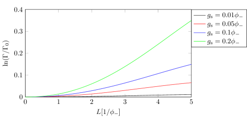
Figure 1: We set $L=T_{0}$ for simplicity and show the change of the modified tunneling rate with increasing $L$ for different couplings $g_{s}$. (For this choice, the exponents in (72) and (79) still remain positive.)

In order to discuss the result quantitatively, we depict in Fig. 1 the dependence of $\ln(\Gamma/\Gamma_{0})$ on the length $L$ which is roughly the size of the nucleating vacuum bubble. The Hubble parameter is set to zero, and we have evaluated $\ln(\Gamma/\Gamma_{0})$ using the exact expressions (3) and (68). Obviously, the correction term of the nucleation rate increases with $L$ and the coupling $g_{\rm s}$. In Fig. 2 we depict the correction term of the exponent in (79) for small values of the Hubble parameter, that is, $L,T_{0}\ll 1/H$. The finite Hubble horizon leads to a reduction of the exponent for small $L$ and $T_{0}$.

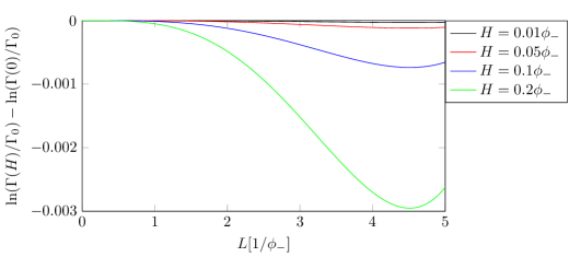
Figure 2: We set $L=T_{0}$ for simplicity and show the change of the modified tunneling rate with increasing $L$ for different Hubble parameters $H$. The coupling was chosen to be $g_{\rm s}=0.1\,\Phi_{-}$.

We note that for unrealistically strong coupling one gets a suppression of the tunneling rate (not shown in the figures); this is reminiscent of the quantum Zeno effect [12, 13]. However, in that limit is may no longer be realistic to neglect the back reaction on the background.

4 Cosmic Landscape

The cosmic landscape motivated by string theory was discussed in various publications [10, 11]. Usually one considers Coleman–De Luccia tunneling [31, 35, 36, 37, 38] between a huge amount of vacua and discusses various solutions of ad hoc rate equations. Under certain circumstances a continuum limit of these rate equations can be derived [39, 40].

Furthermore, finite temperature effects have been considered in [41] based on Hawking–Moss tunneling [42]. Rapid tunneling was proposed under the assumption that resonance tunneling is dominant in the landscape [43, 44, 45], see also [46] for a critics based on standard quantum field theory. In the following, we want to extend our model discussed in the preceding sections to multi-level systems in order to see under which circumstances an ad hoc rate equation can be formulated.

One can, for example, generalize the Hamiltonian (12) in the following way:

$$H_{\phi} = H_{\mathrm{diag}}+H_{\Delta}={\rm diag}(\omega_{1},...,\omega_{n})+\sum_{i\neq j}\Delta_{ij}|i\rangle\langle j|\ ,$$ (80)

$$H_{\mathrm{int}} = g_{\rm s}a^{3}(t){\rm diag}(S_{11},...,S_{nn})\int d^{3}p\,\sigma({\mathbf{p}})\sigma(-{\mathbf{p}})\ .$$ (81)

The interpretation is as follows: The numbers $\omega_{i}$ denote the different local vacua of a cosmic landscape, and the $\Delta_{ij}$ are tunneling matrix elements which can be computed in WKB-approximation. The entries $S_{ii}$ in the interaction Hamiltonian distinguish the different vacua, which is an obvious generalization of measuring the left and the right well in the double-well system discussed above.

Since the tunneling matrix elements are usually exponentially small, the short-time dynamics (short with respect to the tunneling times $\Delta^{-1}_{ij}$) is determined by the decoherence rates. The off-diagonal elements of the density matrix now read, cf. (26),

$$\rho_{ij}(t)=\rho_{ij}(0)\exp\left(-\frac{g_{\rm s}^{2}(S_{ii}-S_{jj})^{2}}{4}\mathrm{Tr}\left(\frac{(\Re\Omega^{{}^{\prime}})^{2}+(\Im\Omega^{{}^{\prime}})^{2}}{(\Re\Omega)^{2}}\right)-i\varphi_{ij}\right)\ .$$ (82)

One can conclude from this expression that the suppression of interference terms depends crucially on the distance between different minima in the landscape.

If one neglects possible degeneracies and assumes that the typical decoherence rate is much larger than the tunneling rate, the system dynamics is determined by the equations [13]

$$\dot{\rho}_{ii}(t)=-\int_{0}^{t}ds[H_{\Delta}(t),[H_{\Delta}(s),\rho(s)]]_{ii}\,.$$ (83)

Applying the Markov approximation, one obtains

$$\dot{\rho}_{ii}(t)=\lambda\sum_{k\neq i}|\Delta_{ik}|^{2}(\rho_{kk}-\rho_{ii})\,,$$ (84)

where $\lambda$ is chosen such that the coarse-graining in time is not too small and the approximation is valid.

There exists another generalization of the model where the tunneling between different vacua may, in fact, be mediated by the environment. This is described by setting $\Delta_{ij}=0$ and $S_{ij}\neq 0,i\neq j$ in the above Hamiltonian. Indirect coupling between metastable states is a well-known phenomena in glasses, see, for example, [47].

In the following we shall derive the master equations for the environment-mediated tunneling. The interaction Hamiltonian in the interaction picture has the form

$$H^{I}_{\rm int}(t)=g_{\rm s}a^{3}(t)\sum_{ij}e^{i(\omega_{i}-\omega_{j})}S_{ij}|i\rangle\langle j|\int d^{3}p\,\sigma(\mathbf{p},t)\sigma(-\mathbf{p},t)\,.$$ (85)

Restricting ourselves to flat slices through de Sitter space, the operators $\sigma(\mathbf{p},t)$ are given by

$$\sigma(\mathbf{p},t)=f_{p}(t)a_{\mathbf{p}}e^{i\mathbf{px}}+{\rm h.c.}$$ (86)

with [22]

$$f_{p}(t)=\sqrt{\frac{V}{(2\pi)^{3}}}\frac{1}{\sqrt{2p^{3}}}\left(\frac{p}{a(t)}+iH\right)e^{i\frac{p}{a(t)H}}\,.$$ (87)

Applying the Redfield approximation [13], we find for the system density matrix the expression

$$\dot{\rho}_{S}^{I}(t)=-\mathrm{Tr}_{B}\int^{t}_{0}ds[H^{I}_{\rm int}(t),[H^{I}_{\rm int}(s),\rho^{I}_{S}(t)\rho_{B}]]\,.$$ (88)

In the limit of vanishing temperature, the bath density matrix is just $\rho_{B}=|0\rangle\langle 0|$. The coefficients of the density matrix satisfy the system of differential equations [48],

$$\dot{\rho}_{ji}^{I}=\delta_{ji}\sum_{k\neq i}\rho_{kk}^{I}(w^{+}_{kiik}+w^{-}_{kiik})-\rho_{ji}^{I}\left[\sum_{l}(w^{+}_{jllj}+w^{-}_{illi})-w^{+}_{iijj}-w^{-}_{iijj}\right]$$ (89)

with the correlation functions

$$w^{+}_{klmn}(t) = g_{\rm s}^{2}\int_{0}^{t}ds\,e^{i(\omega_{k}-\omega_{l})(s-t)}S_{kl}S_{mn}a^{3}(t)a^{3}(s)$$ (90)

$$\times\int d^{3}p\int d^{3}q\langle\sigma(\mathbf{p},s)\sigma(-\mathbf{p},s)\sigma(\mathbf{q},t)\sigma(-\mathbf{q},t)\rangle$$

and

$$w^{-}_{mnkl}(t) = g_{\rm s}^{2}\int_{0}^{t}ds\,e^{i(\omega_{k}-\omega_{l})(s-t)}S_{kl}S_{mn}a^{3}(t)a^{3}(s)$$ (91)

$$\times\int d^{3}p\int d^{3}q\langle\sigma(\mathbf{p},t)\sigma(-\mathbf{p},t)\sigma(\mathbf{q},s)\sigma(-\mathbf{q},s)\rangle\,.$$

In deriving (89), several approximations have been performed: the Born approximation, which states that the total density matrix can be written approximately as a tensor product of the bath density matrix and the system density matrix, and the rotating wave approximation, which is valid when the intrinsic time scale of the system is much larger than the relaxation time of the open system. Since the correlation functions are not homogeneous in time due to the scale factor, the master equation is not Markovian.

The rates in (89) need not be exponentially small and may therefore dominate the dynamics of the string landscape. The transition probabilities between the vacua are symmetric, since we assume that the environment is described by a Gaussian wave function rather than an ensemble of states. On the other hand, the tunneling rates in the Pauli equations (89) are not symmetric and jumping to lower energy levels is more probable than jumping to higher energy levels, depending on the bath temperature. It would be interesting to see how the situation changes if the Gaussian is replaced by a (micro)canonical ensemble.

Evaluating the correlation functions we find

$$w^{+}_{klmn}(t)=g_{\rm s}^{2}\int_{0}^{t}ds\,e^{i(\omega_{k}-\omega_{l})(s-t)}S_{kl}S_{mn}a^{3}(t)a^{3}(s)$$

$$\;\times\frac{(2\pi)^{3}}{V}\int d^{3}k\left(2(f_{k}(t)f^{*}_{k}(s))^{2}+\frac{V}{(2\pi)^{3}}\int d^{3}p|f_{k}(t)|^{2}|f_{p}(s)|^{2}\right)$$ (92)

and

$$w^{-}_{mnkl}(t)=g_{\rm s}^{2}\int_{0}^{t}ds\,e^{i(\omega_{k}-\omega_{l})(s-t)}S_{kl}S_{mn}a^{3}(t)a^{3}(s)$$

$$\;\times\frac{(2\pi)^{3}}{V}\int d^{3}k\left(2(f_{k}(s)f^{*}_{k}(t))^{2}+\frac{V}{(2\pi)^{3}}\int d^{3}p|f_{k}(s)|^{2}|f_{p}(t)|^{2}\right)\,.$$ (93)

The dominating contributions in the correlators (4) and (4) are given by infrared contributions $k<Ha$, since the phases in the integrands are oscillating rapidly if $k>Ha$. Neglecting the second term in the parenthesis of (4), respectively (4), and applying the approximation $e^{ik/Ha}\approx 1$ leads to

$$w^{+}_{klmn}(t) = g_{\rm s}^{2}\int_{0}^{t}ds\,e^{i(\omega_{k}-\omega_{l})(s-t)}S_{kl}S_{mn}a^{3}(t)a^{3}(s)$$ (95)

$$\times\frac{2V}{(2\pi)^{3}}\int d^{3}k\frac{1}{(2k^{3})^{2}}\left(\frac{k}{a(t)}+iH\right)^{2}\left(\frac{k}{a(s)}-iH\right)^{2}$$

and an analogous expression for $w^{-}_{mnkl}(t)$. The evolution equation for the off-diagonal elements read in the Schrödinger picture

$$\dot{\rho}^{\mathrm{Sch}}_{ij}=-(\Gamma_{ij}-i(\omega_{i}-\omega_{j}))\rho_{ij}^{\mathrm{Sch}}$$ (96)

with

$$\Gamma_{ij}=\Re\left(\sum_{l}(w^{+}_{jllj}+w^{-}_{illi})-w^{+}_{iijj}-w^{-}_{iijj}\right)\,.$$ (97)

The imaginary part of the correlation function has been absorbed into the frequencies $\omega_{i}$. For $S_{ij}=S_{ii}\delta_{ij}$ we obtain for $a(t)\gg a(0)$

$$\Gamma_{ij}\approx g_{\rm s}^{2}(S_{ii}-S_{jj})^{2}\frac{VH^{3}a^{6}(t)}{9(2\pi)^{2}}\left(\frac{1}{k_{\mathrm{min}}^{3}}-\frac{1}{k_{\mathrm{max}}^{3}}\right)\ ,$$ (98)

where $k_{\mathrm{min}}$ is an infrared cutoff and $k_{\mathrm{max}}\sim Ha$. Solving (82) using the rates (98) gives for large times

$$|\rho_{ij}(t)| = \rho_{ij}(0)\exp\left(-g_{\rm s}^{2}\int^{t}_{t_{0}}dt^{\prime}\Gamma_{ij}(t^{\prime})\right)$$ (99)

$$\approx \exp\left(-\frac{g_{\rm s}^{2}(S_{ii}-S_{jj})^{2}}{4}\frac{Va^{6}H^{2}}{56\pi^{2}}\left(\frac{1}{k_{\mathrm{min}}^{3}}-\frac{1}{k_{\mathrm{max}}^{3}}\right)\right)\,.$$

This result can be compared with the off-diagonal element (26). Using the dominant contribution of the exponent given by (2.2), we find

$$|\rho_{\pm}(t)|=\rho_{\pm}(0)\exp\left(-g_{\rm s}^{2}\frac{(\phi_{+}-\phi_{-})^{2}}{4}\frac{Va^{6}H^{2}}{56\pi^{2}}\left(\frac{1}{p_{\mathrm{min}}^{3}}-\frac{1}{p_{\mathrm{max}}^{3}}\right)\right)\,,$$ (100)

which coincides with (99) if one identifies $S_{ii}$ ($S_{jj}$) with $\phi_{+}$ ($\phi_{-}$).

The transition between the different localized vacuum states is given by the rate equation

$$\dot{\rho}_{ii}^{\mathrm{Sch}}=-2\sum_{k\neq i}(\Re w_{ikki}^{+}\rho_{ii}^{\mathrm{Sch}}-\Re w_{kiik}^{+}\rho_{kk}^{\mathrm{Sch}})\,.$$ (101)

For $a(t)\gg a(0)$ we find

$$\Re w_{kiik}^{+}=\Re w_{ikki}^{+}=\frac{g_{\rm s}^{2}|S_{ik}|^{2}Va^{6}(t)}{(2\pi)^{2}}\frac{H^{5}}{9H^{2}+(\omega_{i}-\omega_{k})^{2}}\left(\frac{1}{k_{\mathrm{min}}^{3}}-\frac{1}{k_{\mathrm{max}}^{3}}\right)\,.$$ (102)

Depending on the physical situation, that is, depending on whether a bath-induced coupling between different vacua or the tunneling dominates, (101) or (84) describes the evolution of the cosmic landscape.

This evolution is described by $n$ coupled ordinary differential equations and can obviously not be solved for $n\sim 10^{500}$ vacua; therefore, further assumptions and approximations are necessary in order to obtain some physical insight.

The approximation of Markov equations by Fokker–Planck equations is, for example, described in [49] and can always be applied if there is some small expansion parameter, for example, the ratio of the jumps between different vacua and the size of the tunneling landscape. A large number of vacua motivates the transition from discrete values $\rho_{ii}(t)$ to a function $\rho_{x}(t)$, where $x$ is a continuous coordinate in a smooth cosmic landscape. If the landscape is one-dimensional, one might consider the following scenario: There are probabilities to go to the left and to the right, which are described by functions $\alpha(x^{\prime})$ and $\beta(x^{\prime})$ if the observer is located at a position $x^{\prime}$. These functions are the continuum limit next-neighbor transition rates in (84),

$$\lambda|\Delta_{i,i+1}|^{2}=\beta_{i}\rightarrow\beta(x),$$

$$\lambda|\Delta_{i,i-1}|^{2}=\alpha_{i}\rightarrow\alpha(x)\ ,$$ (103)

respectively (101),

$$2\Re w^{+}_{i,i+1,i+1,i}=\beta_{i}\rightarrow\beta(x),$$

$$2\Re w^{+}_{i,i-1,i-1,i}=\alpha_{i}\rightarrow\alpha(x)\,.$$ (104)

The probability that there is a local minimum in the potential between $x$ and $x+dx$ is $\Omega\gamma(x)dx$, where $\Omega$ denotes the size of the cosmic landscape. Therefore, we take into account the tunneling rates and the distance to “nearest neighbors” of local vacua.

The transition from the sum in (101) to a continuous description can be performed as follows:

$$\sum_{k}w^{+}_{kiik}\rho_{kk} =: \sum_{k}w(i,k)\rho(k)$$ (105)

$$= \int dx(\delta(x-k_{1})+...+\delta(x-k_{n}))w(i,x)\rho(x)$$

$$\approx \int dx\int dkf(x-k)w(i,x)\rho(x)$$

$$= \int dx\gamma(x)w(i,x)\rho(x)\,.$$

Following the treatment of [49] and assuming detailed balance,

$$\beta(x^{\prime})\gamma(x)\rho(x^{\prime})_{\mathrm{stat}}=\alpha(x^{\prime})\gamma(x^{\prime})\rho(x)_{\mathrm{stat}}\,,$$ (106)

where $\rho(x)_{\mathrm{stat}}$ is some stationary distribution, the Fokker–Planck equation of diffusion type holds:

$$\frac{\partial\rho(x,t)}{\partial t}=\frac{2}{\Omega}\frac{\partial}{\partial x}\frac{1}{\gamma(x)}\frac{\partial}{\partial x}\frac{\rho(x,t)}{\rho_{\mathrm{stat}}(x)}\,.$$ (107)

This equation describes diffusion in an inhomogeneous medium, since the rates do not prefer a special direction in the cosmic landscape, that is, the dynamics is a random walk in an inhomogeneous medium. The drift term in (107) is due to inhomogeneities in the cosmic landscape and vanishes for $\gamma(x)={\rm const}$. In the following we will rescale the time such that the factor $2/\Omega$ is absorbed. If the rates are time-dependent as in (101), the diffusion equation acquires a time-dependent factor on the right-hand side.

Let us illustrate the solution of (107) in two simple examples. If the pure tunneling given by (84) dominates and $\gamma(x)=\lambda\Delta^{2}$, where $\Delta$ is a typical tunneling rate, we obtain the usual solution for the diffusion equation,

$$\rho(x,t)=\frac{1}{\sqrt{\pi\lambda\Delta^{2}t}}\exp\left(-\frac{x^{2}}{\lambda\Delta^{2}t}\right)\ .$$ (108)

If the dynamics is environment-induced and given by (101), the diffusion depends on the scale factor. For a scalar-field environment and assuming $a(t)=\exp(Ht)$, the result is approximately given by

$$\rho(x,t)=\sqrt{\frac{H}{\pi D(a^{6}-1)}}\exp\left(-\frac{Hx^{2}}{D(a^{6}-1)}\right)\ ,$$ (109)

with

$$D=\frac{g_{\rm s}^{2}L^{3}S^{2}}{H^{2}}\,,$$ (110)

where $S$ denotes a typical transition element $S_{ik}$ in the interaction (81). Therefore the diffusion process may become faster due to the growth of the scale factor. This is, of course, only possible if the cosmic landscape and its environment exchange enough energy to lift the scalar field from one local minima to another.

We have shown in our paper how a small positive value of the cosmological constant could be justified through decoherence. A realistic scenario enabling the calculation of the observed value can, however, only be presented after a definite cosmic landscape for the potential has been retrieved from a fundamental theory.

5 Conclusion and Outlook

In our paper we have addressed the problem why the cosmological constant (dark energy) has a small positive value instead of being exactly zero. Yokoyama had suggested that this could be due to the dark-energy field not being in its ground state (whose energy is assumed to be zero) but in a localized state [9]. Using a quantum mechanical model with a double-well potential, we have justified the localization of the dark-energy field in one of the minima. The crucial mechanism for this is decoherence – the emergence of classical properties (here, a localized state) by irreversible and ubiquitous interaction with irrelevant degrees of freedom (“environment”) leading to quantum entanglement between the dark-energy field and environment [12]. This localization is similar to the emergence of a chiral state for sugar molecules.

More precisely, we have considered a Yukawa interaction between the dark-energy scalar field (quintessence) and environmental modes that can be interpreted as gravitational degrees of freedom. This interaction induces a dynamical suppression of interference terms connecting the two minima. Consequently, the ground state (which is a superposition of the two localized states) will for the dark-energy field evolve into an ensemble of localized states with an effective energy greater than zero. The decoherence factor is dominated by low-frequency super-Hubble modes. These modes become strongly entangled with the dark-energy field because their effective coupling involves an additional factor of $Ha/p$ compared to sub-Hubble modes.

Motivated by recent ideas in string theory, we have generalized our model and have considered an arbitrary number of perturbative vacuum states. Again, strong decoherence leads to the localization in a particular potential well. But one can also obtain the interesting limit of an environment-induced transition between different minima. Within the Markov approximation, we have derived rate equations describing the latter feature. These transitions can dominate the time evolution if the coupling is strong enough to transfer sufficient energy from the environment to the scalar field in order to lift the latter out of the local minima. In the continuum limit we have found the Fokker–Planck equation for the distribution of the dark energy within the landscape of possible vacuum states.

Another issue addressed in our paper is the change of the tunneling rate induced by the coupling to the environment. Is is known from various models involving bilinear couplings between system and environment, for example from the Caldeira–Leggett model [15], that decoherence can lead to the stabilization of metastable states. This is analogous to the quantum Zeno effect, that is, the prevention of a decay process due to the continuous monitoring by the environment.

We have, however, considered in our model a tri- instead of a bilinear coupling and have used a field-theoretical renormalization procedure instead of an ad hoc chosen cutoff frequency. For vacuum bubbles smaller or roughly equal to the Euclidean nucleation time, that is, $L<2\pi T_{0}/3$, we have found an enhancement of the nucleation rate instead of the usual suppression, whereas for $L>2\pi T_{0}/3$ we have found a suppression. The enhancement is a consequence of field theory and similar to the Casimir effect.

Quantum interaction with the environment gives a natural reason for the localization of the dark-energy field in a potential well and, consequently, for a small positive value of the cosmological constant. As long as the precise form of the potential is not known, its exact value can, however, not be computed.

The present work can be extended in various directions. For example, it would be interesting to study the localization process when the dark-energy field is spatially inhomogeneous, that is, when it adopts different values in distinct spatial regions. An additional difficulty would then be the inclusion of collisions between different vacuum bubbles.

Another possible extension would be the application of these ideas to the inflationary era in the early Universe, where the energy scale is much higher. The principal mechanisms of localization and modification of tunneling rates are the same, but the quantitative details are different. From these details one should be able to learn whether or how decoherence can lead to a metastable de Sitter solution and how this could affect the dynamics of the transition to non-inflationary eras following inflation including (re)heating. We hope to return to some of these issues in future publications.

Appendix

In this section we shall give a short review of the $\zeta$-function renormalization method as presented in [32]. The authors there considered the renormalization of a functional determinant defined by a second-order differential equation. Usually, neither the eigenvalues nor the eigenfunctions of the differential operator are known exactly. Moreover, even if all the eigenvalues are known, the determinant is an infinite product of eigenvalues, which is in general a divergent quantity.

To solve these problems, one represents the functional determinant via a generalized Riemann $\zeta$-function. The determinant of an arbitrary differential operator $\mathcal{D}$ can be written as

$$(\mathrm{Det}\mathcal{D})^{1/2}=\exp\left(\frac{1}{2}\ln\prod_{\lambda}\lambda\right)=\exp\left(\frac{1}{2}\sum_{\lambda}\ln\lambda\right)=\exp(W)\,,$$ (111)

where the eigenvalues of the operator are denoted by $\lambda$. We define the generalized $\zeta$-function through

$$\zeta(s)=\sum_{\lambda}\frac{1}{\lambda^{s}}\,,$$ (112)

which is a convergent series for some $s>0$ and can be continued analytically to $s=0$. The exponent $W$ in equation (111) can be obtained through

$$W=-\frac{1}{2}\frac{d}{ds}\zeta(s)\Bigg{|}_{s=0}\,.$$ (113)

Since the eigenvalues of $\mathcal{D}$ have the dimension of mass squared (recall that $\hbar=1$), this leads to a wrong dimensionality for $W$. Therefore we have to replace (113) by

$$W=-\frac{1}{2}\frac{d}{ds}\sum_{\lambda}\left(\frac{\mu^{2}}{\lambda}\right)^{s}\Bigg{|}_{s=0}=-\frac{1}{2}\zeta^{\prime}(0)-\frac{1}{2}\zeta(0)\ln\mu^{2},$$ (114)

where we have introduced a renormalization parameter $\mu$ with mass dimension one.

The differential operator corresponding to a single field mode may be labelled by $n$. In quantum mechanics we are confronted with a finite number of modes, whereas in field theory we have to deal with an infinite number. For each fixed $n$, the eigenvalue equation reads

$$D_{n}u_{n}(-\lambda,t)=\lambda u_{n}(-\lambda,t)\ ,$$ (115)

where $\lambda$ is determined by the boundary condition

$$u_{n}(-\lambda,t_{0})=0\,.$$ (116)

This boundary condition together with a normalization determines the eigenfunctions uniquely. All the boundary conditions (116) can be collected in the equation

$$\mathrm{Det}\,u_{n}(-\lambda,t_{0})=0\ ,$$ (117)

where the determinant is taken with respect to all modes $n$ and all eigenvalues $\lambda$. With the help of the Cauchy formula, the generalized $\zeta$-function can be expressed as

$$\zeta(s)=\frac{1}{2\pi i}\int_{C}\frac{dz}{z^{s}}\frac{d}{dz}\sum_{n}\ln u_{n}(z,t_{0})\ ,$$ (118)

with the contour $C$ encircling all roots of equation (117). Deforming the contour $C$ to a contour $\tilde{C}$ which encircles the branch cut of the function $z^{-s}$, we find

$$\zeta(s)=\frac{\sin(\pi s)}{\pi}\int_{0}^{\infty}\frac{dM^{2}}{M^{2s}}\frac{d}{dM^{2}}\sum_{n}\ln u_{n}(M^{2},t_{0})\,.$$ (119)

We first consider the regularization method for a quantum mechanical system. The necessary information for the regularization of a system with a finite number of modes is contained in the function

$$I(M^{2})=\sum_{n}\ln u_{n}(M^{2},t_{0})\,.$$ (120)

Expanding this function for large $M$ leads to

$$I(M^{2}\rightarrow\infty)=\sum_{k=1}^{N}(I_{k}+\bar{I}_{k}\ln M^{2})M^{2k}+(I^{\mathrm{R}})_{\mathrm{ln}}\ln M^{2}+I^{R}(\infty)\,,$$ (121)

where $(I^{\mathrm{R}})_{\mathrm{ln}}$ is the coefficient of the logarithmic asymptotic term of $I(M^{2})$, and $I^{R}(\infty)$ is the asymptotic value of the regular part of $I(M^{2})$. According to [32], the $\zeta$-function can be expanded as

$$\zeta(s)=(I^{\mathrm{R}})_{\mathrm{ln}}+s[I^{\mathrm{R}}]^{\infty}_{0}+\mathcal{O}(s^{2})\,,$$ (122)

where $[I^{\mathrm{R}}]^{\infty}_{0}=I^{\mathrm{R}}(\infty)-I^{\mathrm{R}}(0)$. As a demonstration we will apply this method to the harmonic oscillator. The eigenvalue equation

$$\left(-\frac{d^{2}}{dt^{2}}+\omega^{2}\right)u(-\lambda,t)=\lambda u(-\lambda,t)\,,\quad u(-\lambda,t_{0})=0\ ,$$ (123)

has a solution of the form

$$u(-\lambda,t)=Ae^{\sqrt{\omega^{2}-\lambda}t}+Be^{-\sqrt{\omega^{2}-\lambda}t}\,.$$ (124)

Performing the analytical continuation to the complex plane, $\lambda\rightarrow z$, the function $u$ adopts on the negative real axis the form

$$u(M^{2},t)=Ae^{\sqrt{\omega^{2}+M^{2}}t}\,,$$ (125)

where we have neglected the exponentially decreasing term. Using for convenience the normalization $u^{\prime}(0)=1$ leads to

$$I(M^{2})=-\frac{1}{2}\ln(\omega^{2}+M^{2})+\sqrt{\omega^{2}+M^{2}}t\,.$$ (126)

Since the term proportional to $\exp(-\sqrt{\omega^{2}+M^{2}}t)$ has been neglected, the analytically continued eigenfunctions do not respect the boundary condition $u(-\lambda,t_{0})=0$.

From (126) we find $I^{\mathrm{R}}(0)=-\ln\omega+\omega t$, $(I^{\mathrm{R}})_{\mathrm{ln}}=-1/2$. Using equations (111), (114), and (122) we arrive at

$$\left(\mathrm{Det}\left[-\frac{d^{2}}{dt^{2}}+\omega^{2}\right]\right)^{-1/2}=\sqrt{\frac{\omega}{\mu}}e^{-\frac{\omega t}{2}}$$ (127)

which gives for large $t$ the correct ground-state energy $\omega/2$ for a harmonic oscillator, cf. Eq. (2.16) in the second reference of [31].

In general, the exact shape of the eigenfunctions $u_{n}(-\lambda,t)$ is unknown and one approximates the $u_{n}$ with a uniform asymptotic WKB-expansion. This asymptotic expansion has the property that

$$\ln u_{n}(M^{2},t_{0})=\phi_{\rm WKB}(n^{2},M^{2}/n^{2})$$ (128)

is uniform for $M^{2}/n^{2}\rightarrow\infty$ and $M^{2}/n^{2}\rightarrow 0$. In addition, it is also possible to use (128) for the regularization of functional determinants in field theory, that is, if the mode number $n$ is not bounded. The expansion (128) has at most a finite power-law order growth in $n$ [32, 50]. This fact allows us to use the parameter $s$ to cure the divergences arising from the infinite number of modes. Changing the integration variable from $M^{2}\rightarrow n^{2}M^{2}$ leads to

$$\zeta(s)=\frac{\sin(\pi s)}{\pi}\int_{0}^{\infty}\frac{dM^{2}}{M^{2s}}\frac{d^{2}}{dM^{2}}I(M^{2},s)\,$$ (129)

with

$$I(M^{2},s)=\sum_{n}\frac{1}{n^{2s}}\ln u_{n}(M^{2}n^{2},t_{0})\,.$$ (130)

For a finite parameter $s>0$ the expression (129) is finite. Analytic continuation of the $\zeta$-function from its convergence domain to $s=0$ leads to [32]

$$\zeta(s) = \frac{1}{s}(I^{\mathrm{pole}})_{\mathrm{ln}}+(I^{\mathrm{R}})_{\mathrm{ln}}+[I^{\mathrm{pole}}]^{\infty}_{0}$$ (131)

$$+s\left\{[I^{\mathrm{R}}]^{\infty}_{0}-\int_{0}^{\infty}dM^{2}\ln M^{2}\frac{dI^{\mathrm{pole}}(M^{2})}{dM^{2}}\right\}+\mathcal{O}(s^{2})\,.$$

The coefficients $(I^{\mathrm{pole}})_{\mathrm{ln}}$, $I^{\mathrm{pole}}(\infty)$ and $I^{\mathrm{R}}(\infty)$ are defined through the large $M$-expansion

$$I(M^{2}\rightarrow\infty,s) = \frac{(I^{\mathrm{pole}})_{\mathrm{ln}}\ln M^{2}+I^{\mathrm{pole}}(\infty)}{s}$$ (132)

$$+I^{\mathrm{R}}(\infty)+(I^{\mathrm{R}})_{\mathrm{ln}}\ln M^{2}+\mathcal{O}(M^{2})\ ,$$

and the pole part $I^{\mathrm{pole}}(M^{2})$ is defined through

$$I(M^{2},s)=\frac{I^{\mathrm{pole}}(M^{2})}{s}+\mathcal{O}(s^{0})\,.$$ (133)

$I^{\mathrm{pole}}(0)$ and $I^{\mathrm{R}}(0)$ are determined by

$$I(M^{2}\rightarrow 0,s)=\frac{I^{\mathrm{pole}}(0)}{s}+I^{\mathrm{R}}(0)+\mathcal{O}(s)\,.$$ (134)

It is also possible to apply the regularization method if the differential equation exhibits singular coefficients. According to Olver [50], the WKB expansion of a second-order differential equation

$$\frac{d^{2}u(M^{2},t)}{dt^{2}}=\omega(t)^{2}u(M^{2},t)=[f(t)+g(t)]u(M^{2},t)$$ (135)

has the form

$$u(M^{2},t)=C(M)(g(t))^{-1/4}\exp\left\{\int_{0}^{t}dt^{\prime}(g(t^{\prime}))^{1/2}\right\}\left[1+h(t)\right]$$ (136)

with $h(t)=\mathcal{O}(M^{-1})$. The function $h(t)$ can be expressed as Volterra integral

$$h(t) = \frac{1}{2}\int^{t}_{t_{0}}\left(1-\exp\left\{2\int^{t^{\prime}}_{0}g^{1/2}(t^{\prime\prime})dt^{\prime\prime}-2\int^{t}_{0}g^{1/2}(t^{\prime})dt^{\prime}\right\}\right)\times$$ (137)

$$\times\psi(t^{\prime})[1+h(t^{\prime})]dt^{\prime}$$

with

$$\psi(t)=\frac{f(t)}{g^{1/2}(t)}-\frac{1}{g^{1/4}(t)}\frac{d^{2}}{dt^{2}}\frac{1}{g^{1/4}(t)}\,.$$ (138)

Therefore the WKB expansion only makes sense if the kernel of (137) is bounded. This leads to the condition

$$\Psi(t)=\int_{t_{0}}^{t}dt^{\prime}|\psi(t^{\prime})|<\infty\ .$$ (139)

Here, $t_{0}$ and $t$ are the boundaries of the interval under consideration. The split of $\omega(t)^{2}$, see (135), is chosen such that singular coefficients like $1/t$ in the differential equation do not destroy the WKB expansion. This is the reason for the $1/4$–trick used in [32].

As already mentioned above, the evaluation of $I(M^{2},s)$ involves an important approximation. In order to fulfill the boundary condition (116), two linearly independent solutions of the corresponding differential equation are required. After analytical continuation, the solutions are of the form $u\sim\exp(Mt)$ and $u\sim\exp(-Mt)$. The second solution is exponentially decreasing and will therefore be discarded. This implies that the analytically continued functions $u(M^{2},t_{0})$ do not respect the boundary condition (116).

References

- [1] E. Komatsu et al., Astrophys. J. Suppl. 192, 18 (2011).
- [2] V. Sahni and A. A. Starobinsky, Int. J. Mod. Phys. D 9, 373 (2000).
- [3] T. Padmanabhan, Phys. Rep. 380, 235 (2003).
- [4] P. J. E. Peebles and B. Ratra, Rev. Mod. Phys. 75, 559 (2003).
- [5] E. J. Copeland, M. Sami, and S. Tsujikawa, Int. J. Mod. Phys. D 15, 1753 (2006).
- [6] V. Sahni and A. A. Starobinsky, Int. J. Mod. Phys. D 15, 2105 (2006).
- [7] J. Frieman, M. Turner, and D. Huterer, Ann. Rev. Astron. Astrophys. 46, 385 (2008).
- [8] C. Kiefer, Quantum Gravity. Second edition (Oxford University Press, Oxford, 2007).
- [9] J. Yokoyama, Phys. Rev. Lett. 88, 15 (2002).
- [10] Universe or Multiverse?, edited by B. Carr (Cambridge University Press, Cambridge, 2007).
- [11] M. R. Douglas, JHEP 05 (2003) 046.
- [12] E. Joos, H. D. Zeh, C. Kiefer, D. Giulini, J. Kupsch, and I.-O. Stamatescu, Decoherence and the Appearance of a Classical World in Quantum Theory, second edition (Springer, Berlin, 2003). See also www.decoherence.de.
- [13] M. Schlosshauer, Decoherence and the Quantum-to-Classical Transition (Springer, Berlin, 2007).
- [14] J. Trost and K. Hornberger, Phys. Rev. Lett. 103, 023202 (2009).
- [15] A. O. Caldeira and A. J. Leggett, Ann. Phys. (N.Y.) 149, 374 (1983).
- [16] S. Capozziello and O. Luongo, arXiv:1010.3347.
- [17] F. S. Queisser, C. Kiefer, and A. A. Starobinsky, In: Proceedings of the Twelfth Marcel Grossmann Conference, Paris, July 2009, to be published.
- [18] V. Mukhanov, Physical Foundations of Cosmology (Cambridge University Press, Cambridge, 2005).
- [19] K. Kuchař, J. Math. Phys. 11, 3322 (1970).
- [20] C. Kiefer, Phys. Rev. D 46, 1658 (1992).
- [21] R. Jackiw, in: Diverse Topics in Theoretical and Mathematical Physics (World Scientific, Singapore, 1995).
- [22] L. Parker and D. Toms, Quantum Field Theory in Curved Spacetime (Cambridge University Press, Cambridge, 2009).
- [23] D. Polarski and A. A. Starobinsky, Class. Quant. Grav. 13, 377 (1996).
- [24] C. Kiefer and D. Polarski, Adv. Sci. Lett. 2, 164 (2009).
- [25] P. R. Anderson, C. Molina-Paris, and E. Mottola, Phys. Rev. D 72, 043515 (2005).
- [26] C. Kiefer, I. Lohmar, D. Polarski, and A. A. Starobinsky, Class. Quant. Grav. 24, 1699 (2007).
- [27] A. Linde, Particle Physics and Inflationary Cosmology (Harwood Academic Publishers, Chur, 1990).
- [28] C. Kiefer, D. Polarski, and A. A. Starobinsky, Int. J. Mod. Phys. D 7, 455 (1998).
- [29] T. Zell, F. Queisser, and R. Klesse, Phys. Rev. Lett. 102, 160501 (2009).
- [30] G. L. Kane, M. J. Perry, and A. N. Żytkow, arXiv:hep-th/0311152v1.
- [31] S. Coleman, Phys. Rev. D 15, 2929 (1977); Aspects of Symmetry (Cambridge University Press, Cambridge, 1985).
- [32] A. O. Barvinsky, A. Yu. Kamenshchik, and I. P. Karmazin, Ann. Phys. (N.Y.) 219, 201 (1992).
- [33] M. A. Evgrafov, Analytic Functions (Dover, New York, 1978).
- [34] A. Barone, M. Gasperini, and G. Rotoli, Phys. Rev. D 82, 087301 (2010).
- [35] S. Coleman and F. de Luccia, Phys. Rev. D 21, 3305 (1980).
- [36] K. Lee and E. J. Weinberg, Phys. Rev. D 36, 1088 (1987).
- [37] T. Clifton, A. Linde, and N. Sivanandam, JHEP 0702 (2007) 024.
- [38] S. Kachru, R. Kallosh, A. Linde, and S. P. Trivedi, Phys. Rev. D 68, 046005 (2003).
- [39] D. Podolsky, J. Majumder, and N. Jokela, JCAP 0805 (2008) 024.
- [40] Y.-S. Piao, arXiv:0810.3654.
- [41] S.-H. H. Tye, D. Wohns, and Y. Zhang, Int. J. Mod. Phys. A 25, 1019 (2010).
- [42] S. W. Hawking and I. L. Moss, Phys. Lett. B 110, 35 (1982).
- [43] S. Sarangi, G. Shiu, and B. Shlaer, Int. J. Mod. Phys. A 24, 741 (2009).
- [44] S.-H. H. Tye, arXiv:hep-th/0611148.
- [45] Q. G. Huang and S.-H. H. Tye, Int. J. Mod. Phys. A 24, 1925 (2009).
- [46] E. J. Copeland, A. Padilla, and P. M. Saffin, JHEP 0801 (2008) 066.
- [47] M. Schechter and P. C. E. Stamp, J. Phys.: Condens. Matter 20, 244136 (2008).
- [48] W. H. Louisell, Quantum statistical properties of radiation (John Wiley & Sons, New York, 1973).
- [49] N. G. van Kampen, Stochastic Processes in Physics and Chemistry (North-Holland Publishing Company, 1981).
- [50] F. W. J. Olver, Asymptotics and Special Functions (Academic Press, New York and London, 1974).