Spin Fidelity for Three-qubit Greenberger-Horne-Zeilinger and W States Under Lorentz Transformations

Abstract

Constructing the reduced density matrix for a system of three massive spin$-\frac{1}{2}$ particles described by a wave packet with Gaussian momentum distribution and a spin part in the form of GHZ or W state, the fidelity for the spin part of the system is investigated from the viewpoint of moving observers in the jargon of special relativity. Using a numerical approach, it turns out that by increasing the boost speed, the spin fidelity decreases and reaches to a non-zero asymptotic value that depends on the momentum distribution and the amount of momentum entanglement.

¹Department of Physics, Faculty of Sciences, University of Isfahan , Isfahan, Iran

²Department of Physics, Faculty of Sciences, Razi University , Kermanshah, Iran

keywords:Wigner rotation, spin density matrix, Gaussian momentum distribution, fidelity, GHZ state, W state.

1 Introduction

The role of special relativity in framing statements about quantum information is illustrated by the fact that quantum entanglement can depend on the reference frame of the observer. In practice, Lorentz transformations can change the entanglement of the spins of massive particles. Relativistic effects on quantum entanglement and quantum information is investigated by many authors. One of the early works in this area has considered a single free spin-$\frac{1}{2}$ particle and by calculating the reduced density matrix, it is shown that the spin entropy is not a relativistic scalar [1]. Alsing and Milborn [2] studied the Lorentz transformation of maximally entangled Bell states. They concluded that entanglement is Lorentz invariant.The entanglement between the spins of a pair of particles may change because the spin and momentum become mixed when viewed by a moving observer [3]. Li an Du have investigated the quantum entanglement between the spins of spin-$\frac{1}{2}$ massive particles in moving frames, for the case that the momenta of the particles are entangled [4]. They have shown that, if the momenta of the pair are appropriately entangled, the entanglement between the spins of the Bell states remains maximal when viewed from any Lorentz-transformed frame. Bartlett and Terno showed that relativistically invariant quantum information can be encoded into states of indistinguishable particles [5]. Recently, simple examples have been presented of Lorentz transformation that entangle the spins and momenta of two spin-$\frac{1}{2}$ particles with positive mass such that no sum of entanglements have been found to be unchanged [6]. Fidelity for the spin part of a system of two spin$-\frac{1}{2}$ particles described by a Gaussian momentum distributed wave packet is studied from the view point of moving observers and it is shown that the fidelity decreases by increasing the boost velocity [7]. Bell’s inequality in moving frames has been considered in several papers [8, 9, 10, 11, 12, 13]. The degree of violation of Bell’s inequality will decrease with increasing the velocity of the observers if the directions of the measurements are fixed. However, this doesn’t imply a breakdown of nonlocal correlation since the perfect anti-correlation is maintained in the appropriately chosen different directions. Some efforts have been done for extending these ideas to tripartite systems. For example, Lorentz transformation of three-qubit GHZ state is studied and it is shown that Bell’s inequality is maximally violated for this state [14]. In tripartite discrete systems, two classes of genuine tripartite entanglement have been discovered, namely, the Greenberger-Horne-Zeilinger (GHZ) class [15, 16] and the W class [17, 18]. Some authors have provided proposals for generation and observation of GHZ or W type entanglements [19, 20, 21, 22, 23].

In this paper we consider a moving system containing three spin-$\frac{1}{2}$ massive particles such that in the rest frame, its spin part be entangled as one of the GHZ or W states. In the present approach, we introduce a Gaussian momentum distributed wave packet represented in the momentum space for the system as viewed in the rest frame. Also we introduce the wave packet for the system as viewed by a boosted observer. Then we focus on the spin part of each wave packet by finding the corresponding reduced density matrix. As a result of relativistic spin decoherence, the reduced density matrix observed in the boosted frame is mixed even though it is prepared to be pure in the rest frame. We quantify the amount of mixing via calculating the fidelity for these two reduced density matrices. We will consider general boosts in the $xz$-plane. To see the effect of momentum entanglement on the results, the momentum part is chosen to be in extreme cases of momentum product or momentum perfectly correlated.

2 Lorentz transformation of reduced density matrix

A three-particle quantum state is expressed by

$$|\textbf{p}_{1},\sigma_{1};\textbf{p}_{2},\sigma_{2};\textbf{p}_{3},\sigma_{3}\rangle=a^{\dagger}(\textbf{p}_{1},\sigma_{1})a^{\dagger}(\textbf{p}_{2},\sigma_{2})a^{\dagger}(\textbf{p}_{3},\sigma_{3})|\Phi_{0}\rangle,$$ (1)

where p is the 3-momentum vector, $\sigma$ is the spin label, $a^{\dagger}$ is creation operator and $|\Phi_{0}\rangle$ is the Lorentz invariant vacuum state. The state (1) has a Lorentz transformation property [24] as

$$U(\Lambda)|\textbf{p}_{1},\sigma_{1};\textbf{p}_{2},\sigma_{2};\textbf{p}_{3},\sigma_{3}\rangle = \sum_{\sigma^{\prime}_{1}\sigma^{\prime}_{2}\sigma^{\prime}_{3}}D_{\sigma^{\prime}_{1}\sigma_{1}}(W(\Lambda,p_{1}))D_{\sigma^{\prime}_{2}\sigma_{2}}(W(\Lambda,p_{2}))D_{\sigma^{\prime}_{3}\sigma_{3}}(W(\Lambda,p_{3}))$$

$$\times|\Lambda\textbf{p}_{1},\sigma^{\prime}_{1};\Lambda\textbf{p}_{2},\sigma^{\prime}_{2};\Lambda\textbf{p}_{3},\sigma^{\prime}_{3}\rangle,$$

where $\Lambda\textbf{p}$ is the spatial part of $\Lambda p$, $D_{\sigma^{\prime}\sigma}(W(\Lambda,p))$ is the unitary representation of the Wigner rotation operator, and $W(\Lambda,p)$ is the Wigner’s little group element

$$W(\Lambda,p)=L^{-1}(\Lambda p)\Lambda L(p),$$ (3)

where $L(p)$ is the standard boost that takes a massive particle of mass $m$ from rest to a 4-momentum $p$. The transformation of the creation operator is as

$$U(\Lambda)a^{\dagger}(\textbf{p},\sigma)U^{-1}(\Lambda)=\sum_{\sigma^{\prime}}D_{\sigma^{\prime}\sigma}(W(\Lambda,p))a^{\dagger}({\Lambda}\textbf{p},\sigma^{\prime}).$$ (4)

Let $\hat{\textbf{p}}$ be the unit vector along the 3-momentum of a particle as viewed in the rest frame, and consider a boost along $\hat{\textbf{e}}$ with speed $V$. Then, the Wigner rotation operator is represented as

$$D(W(\Lambda,p))={\bf 1}\cos\frac{\Omega}{2}+i({\bf\sigma}\cdot\hat{\textbf{n}})\sin\frac{\Omega}{2},$$ (5)

where ${\bf 1}$ is the unit $2\times 2$ matrix, ${\bf\sigma}=\left(\sigma_{1},\sigma_{2},\sigma_{3}\right)$ denotes the Pauli matrices, $\hat{\textbf{n}}=\frac{\hat{\textbf{e}}\times\hat{\textbf{p}}}{|\hat{\textbf{e}}\times\hat{\textbf{p}}|}$ and

$$\cot\frac{\Omega}{2}=\frac{\coth\frac{\xi}{2}\coth\frac{\eta}{2}+\hat{\textbf{e}}\cdot\hat{\textbf{p}}}{|\hat{\textbf{e}}\times\hat{\textbf{p}}|},$$ (6)

where

$$\cosh\xi=\frac{p^{0}}{m},\,\,\,\,\,\,\,\,\,\,\,\,\,\,\,\tanh\eta=\frac{V}{c}.$$ (7)

In the rest frame of the observer, the 4-momentum of each particle can be written in polar coordinates as

$$p^{\mu}=[mc\,\cosh\xi,mc\sinh\,\xi(\cos\varphi\sin\vartheta,\sin\varphi\sin\vartheta,\cos\vartheta)],$$ (8)

where $\tanh\xi=\frac{v}{c}$ and $v$ is the speed of the particle. To be specific, we suppose that particles are moving along the positive $x$-axis, i.e., $\vartheta=\frac{\pi}{2}$ and $\varphi=0$, then the 4-momentum reduces to

$$p^{\mu}=(mc\cosh\xi,mc\sinh\xi,0,0).$$ (9)

This means that all of the three particles are assumed move along the positive $x$-axis, so for an arbitrary boost direction $\hat{\textbf{e}}=(\cos\phi\sin\theta,\sin\phi\sin\theta,\cos\theta)$, the axis of Wigner rotation $\hat{\textbf{n}}$ is perpendicular to the $x$-axis in the same one direction for all three particles. We will consider only $\phi=0$.

In this case the boost direction lies in the $xz$-plane and the Wigner rotation is about the $y$-axis as

$$D(W(\Lambda,p))=\left(\begin{array}[]{cc}D_{\uparrow\uparrow}(\Omega)&D_{\uparrow\downarrow}(\Omega)\\ D_{\downarrow\uparrow}(\Omega)&D_{\downarrow\downarrow}(\Omega)\\ \end{array}\right)=\left(\begin{array}[]{cc}\cos\frac{\Omega}{2}&\sin\frac{\Omega}{2}\\ -\sin\frac{\Omega}{2}&\cos\frac{\Omega}{2}\\ \end{array}\right)$$ (14)

where

$$\cot\frac{\Omega}{2}=\frac{\coth\frac{\xi}{2}\coth\frac{\eta}{2}+\sin\theta}{\cos\theta},$$ (15)

One may provide the argument using 3-particle states (1) and (2) which require a sharp momentum distribution around momentum p for each particle. But the realistic situation involves a wave packet of the system with a definite momentum distribution. We follow the argument in terms of Gaussian momentum distributed wave packets.

In the rest frame of an observer the wave packet in momentum representation for the 3-particle system generally can be expressed as

$$|\psi\rangle=\sum_{\sigma_{1}\sigma_{2}\sigma_{3}}\int\int\int d^{3}{\textbf{p}}_{1}d^{3}{\textbf{p}}_{2}d^{3}{\textbf{p}}_{3}\,g_{\sigma_{1}\sigma_{2}\sigma_{3}}({\textbf{p}}_{1},{\textbf{p}}_{2},{\textbf{p}}_{3})|{\textbf{p}}_{1},\sigma_{1};{\textbf{p}}_{2},\sigma_{2};{\textbf{p}}_{3},\sigma_{3}\rangle,$$ (16)

where $g_{\sigma_{1}\sigma_{2}\sigma_{3}}({\textbf{p}}_{1},{\textbf{p}}_{2},{\textbf{p}}_{3})$ is a distribution function for momentum and spin that is normalized as

$$\sum_{\sigma_{1}\sigma_{2}\sigma_{3}}\int\int\int d^{3}{\textbf{p}}_{1}d^{3}{\textbf{p}}_{2}d^{3}{\textbf{p}}_{3}|g_{\sigma_{1}\sigma_{2}\sigma_{3}}({\textbf{p}}_{1},{\textbf{p}}_{2},{\textbf{p}}_{3})|^{2}=1,$$ (17)

which makes to have

$$\langle{\textbf{p}}^{\prime}_{1},\sigma^{\prime}_{1};{\textbf{p}}^{\prime}_{2},\sigma^{\prime}_{2};{\textbf{p}}^{\prime}_{3},\sigma^{\prime}_{3}|{\textbf{p}}_{1},\sigma_{1};{\textbf{p}}_{2},\sigma_{2};{\textbf{p}}_{3},\sigma_{3}\rangle=\delta^{3}({\textbf{p}}^{\prime}_{1}-{\textbf{p}}_{1})\delta^{3}({\textbf{p}}^{\prime}_{2}-{\textbf{p}}_{2})\delta^{3}({\textbf{p}}^{\prime}_{3}-{\textbf{p}}_{3})\delta_{\sigma^{\prime}_{1}\sigma_{1}}\delta_{\sigma^{\prime}_{2}\sigma_{2}}\delta_{\sigma^{\prime}_{3}\sigma_{3}}.$$ (18)

Now, regarding (2), for a boosted observer the state (16) changes to

$$|\psi^{b}\rangle = \sum_{\sigma_{1}\sigma_{2}\sigma_{3}}\sum_{\sigma^{\prime}_{1}\sigma^{\prime}_{2}\sigma^{\prime}_{3}}\int d^{3}{\textbf{p}}_{1}\int d^{3}{\textbf{p}}_{2}\int d^{3}{\textbf{p}}_{3}\sqrt{\frac{(\Lambda p_{1})^{0}}{p_{1}^{0}}}\sqrt{\frac{(\Lambda p_{2})^{0}}{p_{2}^{0}}}\sqrt{\frac{(\Lambda p_{3})^{0}}{p_{3}^{0}}}g_{\sigma_{1}\sigma_{2}\sigma_{3}}({\textbf{p}}_{1},{\textbf{p}}_{2},{\textbf{p}}_{3})$$

$$\times D_{\sigma^{\prime}_{1}\sigma_{1}}(W(\Lambda,p_{1}))D_{\sigma^{\prime}_{2}\sigma_{2}}(W(\Lambda,p_{2}))D_{\sigma^{\prime}_{3}\sigma_{3}}(W(\Lambda,p_{3}))|\Lambda\textbf{p}_{1},\sigma^{\prime}_{1};\Lambda\textbf{p}_{2},\sigma^{\prime}_{2};\Lambda\textbf{p}_{3},\sigma^{\prime}_{3}\rangle,$$

where $D_{\sigma^{\prime}_{i}\sigma_{i}}$ is given by (14).

The density operators corresponding to these pure states are $\rho=|\psi\rangle\langle\psi|$ and $\rho^{b}=|\psi^{b}\rangle\langle\psi^{b}|$, however we need the reduced density operators $\varrho$ and $\varrho^{b}$ obtained by tracing over the momentum of the density operators, that is

$$\varrho_{\sigma^{\prime}_{1}\sigma^{\prime}_{2}\sigma^{\prime}_{3},\sigma_{1}\sigma_{2}\sigma_{3}}=\int\int\int d^{3}{\textbf{p}}_{1}d^{3}{\textbf{p}}_{2}d^{3}{\textbf{p}}_{3}\,g_{\sigma^{\prime}_{1}\sigma^{\prime}_{2}\sigma^{\prime}_{3}}({\textbf{p}}_{1},{\textbf{p}}_{2},{\textbf{p}}_{3})g^{*}_{\sigma_{1}\sigma_{2}\sigma_{3}}({\textbf{p}}_{1},{\textbf{p}}_{2},{\textbf{p}}_{3}),$$ (20)

and

$$\varrho^{b}_{\sigma^{\prime}_{1}\sigma^{\prime}_{2}\sigma^{\prime}_{3},\sigma_{1}\sigma_{2}\sigma_{3}} = \sum_{\sigma^{\prime\prime}_{1}\sigma^{\prime\prime}_{2}\sigma^{\prime\prime}_{3}}\sum_{\sigma^{\prime\prime\prime}_{1}\sigma^{\prime\prime\prime}_{2}\sigma^{\prime\prime\prime}_{3}}\int\int\int d^{3}{\textbf{p}}_{1}d^{3}{\textbf{p}}_{2}d^{3}{\textbf{p}}_{3}$$

$$\times\left[D_{\sigma^{\prime}_{1}\sigma^{\prime\prime}_{1}}(W(\Lambda_{1},p_{1}))D_{\sigma^{\prime}_{2}\sigma^{\prime\prime}_{2}}(W(\Lambda_{2},p_{2}))D_{\sigma^{\prime}_{3}\sigma^{\prime\prime}_{3}}(W(\Lambda_{3},p_{3}))g_{\sigma^{\prime\prime}_{1}\sigma^{\prime\prime}_{2}\sigma^{\prime\prime}_{3}}({\textbf{p}}_{1},{\textbf{p}}_{2},{\textbf{p}}_{3})\right]$$

$$\times\left[D_{\sigma_{1}\sigma^{\prime\prime\prime}_{1}}(W(\Lambda_{1},p_{1}))D_{\sigma_{2}\sigma^{\prime\prime\prime}_{2}}(W(\Lambda_{2},p_{2}))D_{\sigma_{3}\sigma^{\prime\prime\prime}_{3}}(W(\Lambda_{3},p_{3}))g_{\sigma^{\prime\prime\prime}_{1}\sigma^{\prime\prime\prime}_{2}\sigma^{\prime\prime\prime}_{3}}({\textbf{p}}_{1},{\textbf{p}}_{2},{\textbf{p}}_{3})\right]^{*}.$$

Clearly $\varrho^{b}$ denotes the Lorentz transformed form of $\varrho$. It must be noted that $\varrho^{b}$ will be mixed even if $\varrho$ is pure.

Our purpose here is to calculate the fidelity of $\varrho$ and $\varrho^{b}$, which accordingly we call it the spin fidelity $F_{s}$. Then, we use the Uhlmann definition [25, 26] for fidelity of mixed states, that is

$$F_{s}=\left[\textrm{Tr}(\sqrt{\sqrt{\varrho}\,\varrho^{b}\sqrt{\varrho}})\right]^{2}.$$ (22)

Fidelity is a basic ingredient in communication theory and for any given communication scheme it is a quantitative measure of the accuracy of the transmission. It takes numbers between 0 and 1; a perfect communication corresponds to the fidelity 1. In the present argument the spin fidelity quantify how $\varrho^{b}$ looks like $\varrho$.

Recall that in our problem each 3-momentum has only one component along the $x$-axis. Then all the three-dimensional integrals reduce to one-dimensional integrals where the bold notation for the momenta is suppressed. In the following $p$ stands for the $x$-component of 3-momentum, not for the 4-momentum.

Now we choose the distribution function $g_{\sigma_{1}\sigma_{2}\sigma_{3}}(p_{1},p_{2},p_{3})$ such that the spin and the momentum parts be separable and assume that the spin part is in GHZ or W state. In tripartite discrete systems, two classes of genuine tripartite entanglement have been discovered, namely, the GHZ class [15, 16] and the W class [17, 18]. These two different types of entanglement are not equivalent and cannot be converted to each other by local unitary operations combined with classical communication. In terms of the spin basis, the GHZ state has the form $|\textrm{GHZ}\rangle=\frac{1}{\sqrt{2}}\left(|\uparrow\uparrow\uparrow\rangle+|\downarrow\downarrow\downarrow\rangle\right)$ and the W state takes the form $|\textrm{W}\rangle=\frac{1}{\sqrt{3}}\left(|\uparrow\downarrow\downarrow\rangle+|\downarrow\uparrow\downarrow\rangle+|\downarrow\downarrow\uparrow\rangle\right)$. The entanglement in the W state is robust against the loss of one qubit, while the GHZ state is reduced to a product of two qubits. According to the geometric measure of entanglement, the W state has higher entanglement than the GHZ state does [27]. Methods are proposed for generation and observation of GHZ or W type entanglements [22, 23]. In our argument, it becomes apparent that there is an interesting contrast between the behavior of spin fidelity for these two states.

3 GHZ state

In this section we specify $g_{\sigma_{1}\sigma_{2}\sigma_{3}}(p_{1},p_{2},p_{3})$ such that in the rest frame the spin part of the wave packet be in the GHZ state and, to perceive the effect of momentum correlation on the results, the momentum part be in states with different momentum correlation.

First we choose the distribution function as

$$g_{\sigma_{1}\sigma_{2}\sigma_{3}}(p_{1},p_{2},p_{3})=f(p_{1})f(p_{2})f(p_{3})\frac{1}{\sqrt{2}}\left(\delta_{\sigma_{1}\uparrow}\delta_{\sigma_{2}\uparrow}\delta_{\sigma_{3}\uparrow}+\delta_{\sigma_{1}\downarrow}\delta_{\sigma_{2}\downarrow}\delta_{\sigma_{3}\downarrow}\right),$$ (23)

which as applied in (16), evidently gives a state that its spin part is entangled as the GHZ state and the momentum part is separable, i.e., the momentum entanglement is zero. We refer to this choice as the momentum product case. For evaluating the integrals, we should pick out a specified form for $f(p)$. Here we consider it as

$$f(p)=\frac{2}{(\alpha^{2}\pi)^{\frac{1}{4}}}\exp\left[-\frac{1}{2}\left(\frac{p}{\alpha}\right)^{2}\right],$$ (24)

which shows a Gaussian distribution (minimum uncertainty) of momentum around $p=0$ with a width determined by $\alpha$. Applying (23) in (20) and (2) we get

$$\varrho=\frac{1}{2}\left(\begin{array}[]{cccccccc}1&0&0&0&0&0&0&1\\ 0&0&0&0&0&0&0&0\\ 0&0&0&0&0&0&0&0\\ 0&0&0&0&0&0&0&0\\ 0&0&0&0&0&0&0&0\\ 0&0&0&0&0&0&0&0\\ 0&0&0&0&0&0&0&0\\ 1&0&0&0&0&0&0&1\\ \end{array}\right),$$ (25)

which is pure and

$$\varrho^{b}_{\sigma^{\prime}_{1}\sigma^{\prime}_{2}\sigma^{\prime}_{3},\sigma_{1}\sigma_{2}\sigma_{3}} = \frac{1}{2}\int dp_{1}|f(p_{1})|^{2}\int dp_{2}|f(p_{2})|^{2}\int dp_{3}|f(p_{3})|^{2}$$

$$\times[D_{\sigma^{\prime}_{1}\uparrow}(\Omega_{1})D_{\sigma^{\prime}_{2}\uparrow}(\Omega_{2})D_{\sigma^{\prime}_{3}\uparrow}(\Omega_{3})D^{*}_{\sigma_{1}\uparrow}(\Omega_{1})D^{*}_{\sigma_{2}\uparrow}(\Omega_{2})D^{*}_{\sigma_{3}\uparrow}(\Omega_{3})$$

$$+D_{\sigma^{\prime}_{1}\uparrow}(\Omega_{1})D_{\sigma^{\prime}_{2}\uparrow}(\Omega_{2})D_{\sigma^{\prime}_{3}\uparrow}(\Omega_{3})D^{*}_{\sigma_{1}\downarrow}(\Omega_{1})D^{*}_{\sigma_{2}\downarrow}(\Omega_{2})D^{*}_{\sigma_{3}\downarrow}(\Omega_{3})$$

$$+D_{\sigma^{\prime}_{1}\downarrow}(\Omega_{1})D_{\sigma^{\prime}_{2}\downarrow}(\Omega_{2})D_{\sigma^{\prime}_{3}\downarrow}(\Omega_{3})D^{*}_{\sigma_{1}\uparrow}(\Omega_{1})D^{*}_{\sigma_{2}\uparrow}(\Omega_{2})D^{*}_{\sigma_{3}\uparrow}(\Omega_{3})$$

$$+D_{\sigma^{\prime}_{1}\downarrow}(\Omega_{1})D_{\sigma^{\prime}_{2}\downarrow}(\Omega_{2})D_{\sigma^{\prime}_{3}\downarrow}(\Omega_{3})D^{*}_{\sigma_{1}\downarrow}(\Omega_{1})D^{*}_{\sigma_{2}\downarrow}(\Omega_{2})D^{*}_{\sigma_{3}\downarrow}(\Omega_{3})],$$

which is mixed. Since $\varrho$ is pure $\varrho^{2}=\varrho$ and (22) can be written as

$$F_{s}=\left[\textrm{Tr}(\sqrt{\varrho\,\varrho^{b}\varrho})\right]^{2}.$$ (27)

Using (25) and (3) in (27), the spin fidelity is obtained as

$$F_{s}=\frac{1}{2}\left(\varrho^{b}_{\uparrow\uparrow\uparrow,\uparrow\uparrow\uparrow}+\varrho^{b}_{\uparrow\uparrow\uparrow,\downarrow\downarrow\downarrow}+\varrho^{b}_{\downarrow\downarrow\downarrow,\uparrow\uparrow\uparrow}+\varrho^{b}_{\downarrow\downarrow\downarrow,\downarrow\downarrow\downarrow}\right).$$ (28)

We apply the Wigner rotation (14) in (3), then we obtain

$$F_{s} = \frac{1}{8}[\,\overline{\cos\Omega_{1}}\,\,\overline{\cos\Omega_{2}}\,\,\overline{\cos\Omega_{3}}+\overline{\cos\Omega_{1}}\,\,\overline{\cos\Omega_{2}}+\overline{\cos\Omega_{1}}\,\,\overline{\cos\Omega_{3}}$$

$$+\overline{\cos\Omega_{2}}\,\,\overline{\cos\Omega_{3}}+\overline{\cos\Omega_{1}}+\overline{\cos\Omega_{2}}+\overline{\cos\Omega_{3}}+1],$$

where for each particle

$$\overline{\cos\Omega}=\frac{2}{\gamma\sqrt{\pi}}\int_{0}^{\infty}d\xi\,e^{-\gamma^{-2}\sinh^{2}\xi}\cosh\xi\left[1-\frac{\cos^{2}\theta\left(1+\cosh\eta\cosh\xi-\cosh\eta-\cosh\xi\right)}{1+\cosh\eta\cosh\xi+\sin\theta\sinh\eta\sinh\xi}\right],$$ (30)

where $\gamma=\alpha/mc$, $\sinh\xi=p/mc$ and we have used (15) and (24). Note that $\overline{\cos\Omega_{1}}=\overline{\cos\Omega_{2}}=\overline{\cos\Omega_{3}}$, then spin fidelity (3) reduces to

$$F_{s}=\frac{1}{8}\left(\overline{\cos\Omega}^{\,\,3}+3\overline{\cos\Omega}^{\,\,2}+3\overline{\cos\Omega}+1\right).$$ (31)

Next, we consider a case that two of three momenta, say $p_{2}$ and $p_{3}$ are perfectly correlated. We refer to it as the 2-momentum correlated case. Thus we write

$$g_{\sigma_{1}\sigma_{2}\sigma_{3}}(p_{1},p_{2},p_{3})=f(p_{1})f(p_{2})\sqrt{\delta(p_{2}-p_{3})}\frac{1}{\sqrt{2}}\left(\delta_{\sigma_{1}\uparrow}\delta_{\sigma_{2}\uparrow}\delta_{\sigma_{3}\uparrow}+\delta_{\sigma_{1}\downarrow}\delta_{\sigma_{2}\downarrow}\delta_{\sigma_{3}\downarrow}\right),$$ (32)

which as substituted in (20) and (2) gives a pure $\varrho$ as (25) and a mixed $\varrho^{b}$. Applying the results in (27), we have

$$F_{s}=\frac{1}{8}\left(\,\,\overline{\cos\Omega_{1}}\,\,\overline{\cos^{2}\Omega_{2}}+2\,\,\overline{\cos\Omega_{1}}\,\,\overline{\cos\Omega_{2}}+\overline{\cos^{2}\Omega_{2}}+\overline{\cos\Omega_{1}}+2\,\,\overline{\cos\Omega_{2}}+1\right),$$ (33)

which is comparable with (3). Again note that $\overline{\cos\Omega_{1}}=\overline{\cos\Omega_{2}}$, then

$$F_{s}=\frac{1}{8}\left(\overline{\cos\Omega}\,\,\overline{\cos^{2}\Omega}+2\,\,\overline{\cos\Omega}^{\,\,2}+\overline{\cos^{2}\Omega}+3\overline{\cos\Omega}+1\right),$$ (34)

where

$$\overline{\cos^{2}\Omega}=\frac{2}{\gamma\sqrt{\pi}}\int_{0}^{\infty}d\xi\,e^{-\gamma^{-2}\sinh^{2}\xi}\cosh\xi\left[1-\frac{\cos^{2}\theta\left(1+\cosh\eta\cosh\xi-\cosh\eta-\cosh\xi\right)}{1+\cosh\eta\cosh\xi+\sin\theta\sinh\eta\sinh\xi}\right]^{2}.$$ (35)

Here we note that, in (32) as well as in the following arguments, the delta functions should be regarded as limits of analytical functions under certain conditions. Precisely, perfectly correlated momenta should be regarded as a limiting case of entangled Gaussian momenta [4]. An experimental situation for generating the momentum entanglement is discussed by Lamata et.al. [28]. They studied the dynamics of momentum entanglement generated in the lowest-order QED interaction between two massive spin-$\frac{1}{2}$ charged particles, which grows in time as the two fermions exchange virtual photons. In this scheme the degree of generated entanglement between interacting particles with initial well-defined momentum can be infinite, however, they explained this divergence in the context of entanglement theory for continuous variables, and showed how to circumvent this apparent paradox.

In order to have all the three momenta perfectly correlated ( 3-momentum correlated case) we choose

$$g_{\sigma_{1}\sigma_{2}\sigma_{3}}(p_{1},p_{2},p_{3}) = f(p_{1})\sqrt{\delta(p_{1}-p_{2})\delta(p_{1}-p_{3})}$$

$$\times\frac{1}{\sqrt{2}}(\delta_{\sigma_{1}\uparrow}\delta_{\sigma_{2}\uparrow}\delta_{\sigma_{3}\uparrow}+\delta_{\sigma_{1}\downarrow}\delta_{\sigma_{2}\downarrow}\delta_{\sigma_{3}\downarrow}),$$

which as substituted in (20) and (2), gives

$$F_{s}=\frac{1}{8}\left(\overline{\cos^{3}\Omega}+3\overline{\cos^{2}\Omega}+3\overline{\cos\Omega}+1\right),$$ (37)

where

$$\overline{\cos^{3}\Omega}=\frac{2}{\gamma\sqrt{\pi}}\int_{0}^{\infty}d\xi\,e^{-\gamma^{-2}\sinh^{2}\xi}\cosh\xi\left[1-\frac{\cos^{2}\theta\left(1+\cosh\eta\cosh\xi-\cosh\eta-\cosh\xi\right)}{1+\cosh\eta\cosh\xi+\sin\theta\sinh\eta\sinh\xi}\right]^{3},$$ (38)

There is no analytical solution for the integrals (30), (35) and (38) hence we switch to a numerical approach for evaluating the spin fidelity $F_{s}$. It reveals that the behavior of $F_{s}$ in terms of the boost velocity is in the same form for all the $\theta$’s and the most change occurs for $\theta=0$, that is, when the boost is along the $z$-axis. Therefore, we proceed with substituting $\theta=0$ in the integrals. Fig. 1 shows $F_{s}$ plotted numerically in terms of the boost parameter $\eta$ for a given width for the momentum distribution. The solid curve shows $F_{s}$ given by (31) in the momentum product case. The dashed curve is plotted for $F_{s}$ given by (33) in the 2-momentum correlated case and the dashed-dotted curve is for $F_{s}$ given by (37) in the 3-momentum correlated case. We see that by increasing the boost velocity more spin decoherence occurs and expectedly the spin fidelity decreases with increasing $\eta$. By increasing the momentum correlation, $F_{s}$ decreases less, such that for small $\eta$ the curves coincide, and for $\eta\rightarrow\infty$ (ultra relativistic limit) they slightly split to non-zero asymptotic values. It can be shown that by decreasing the width $\gamma$, the spin fidelity becomes less sensitive to $\eta$, hence the slope of the curves decreases.

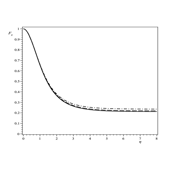
Figure 1: Spin fidelity $F_{s}$ versus the boost parameter $\eta$ in the GHZ case plotted for $\gamma=20$. The solid curve is plotted for the momentum product (zero momentum entanglement) while the dashed and the dashed-dotted correspond to the 2-momentum correlated and 3-momentum correlated cases, respectively. For small $\eta$ the curves coincide however at large $\eta$ they slightly split.

4 W state

As the previous section we investigate the W state in three cases of different momentum correlation. We begin with the momentum product case, by choosing

$$g_{\sigma_{1}\sigma_{2}\sigma_{3}}(p_{1},p_{2},p_{3})=f(p_{1})f(p_{2})f(p_{3})\frac{1}{\sqrt{3}}\left(\delta_{\sigma_{1}\uparrow}\delta_{\sigma_{2}\downarrow}\delta_{\sigma_{3}\downarrow}+\delta_{\sigma_{1}\downarrow}\delta_{\sigma_{2}\uparrow}\delta_{\sigma_{3}\downarrow}+\delta_{\sigma_{1}\downarrow}\delta_{\sigma_{2}\downarrow}\delta_{\sigma_{3}\uparrow}\right).$$ (39)

By this choice (20) leads to

$$\varrho=\frac{1}{3}\left(\begin{array}[]{cccccccc}0&0&0&0&0&0&0&0\\ 0&0&0&0&0&0&0&0\\ 0&0&0&0&0&0&0&0\\ 0&0&0&1&0&1&1&0\\ 0&0&0&0&0&0&0&0\\ 0&0&0&1&0&1&1&0\\ 0&0&0&1&0&1&1&0\\ 0&0&0&0&0&0&0&0\\ \end{array}\right),$$ (40)

which is pure and (2) gives

$$\varrho^{b}_{\sigma^{\prime}_{1}\sigma^{\prime}_{2}\sigma^{\prime}_{3},\sigma_{1}\sigma_{2}\sigma_{3}}=\frac{1}{3}\int dp_{1}|f(p_{1})|^{2}\int dp_{2}|f(p_{2})|^{2}\int dp_{3}|f(p_{3})|^{2}$$ (41)

$$\times[D_{\sigma^{\prime}_{1}\uparrow}(\Omega_{1})D_{\sigma^{\prime}_{2}\downarrow}(\Omega_{2})D_{\sigma^{\prime}_{3}\downarrow}(\Omega_{3})+D_{\sigma^{\prime}_{1}\downarrow}(\Omega_{1})D_{\sigma^{\prime}_{2}\uparrow}(\Omega_{2})D_{\sigma^{\prime}_{3}\downarrow}(\Omega_{3})+D_{\sigma^{\prime}_{1}\downarrow}(\Omega_{1})D_{\sigma^{\prime}_{2}\downarrow}(\Omega_{2})D_{\sigma^{\prime}_{3}\uparrow}(\Omega_{3})]$$

$$\times[D_{\sigma_{1}\uparrow}(\Omega_{1})D_{\sigma_{2}\downarrow}(\Omega_{2})D_{\sigma_{3}\downarrow}(\Omega_{3})+D_{\sigma_{1}\downarrow}(\Omega_{1})D_{\sigma_{2}\uparrow}(\Omega_{2})D_{\sigma_{3}\downarrow}(\Omega_{3})+D_{\sigma_{1}\downarrow}(\Omega_{1})D_{\sigma_{2}\downarrow}(\Omega_{2})D_{\sigma_{3}\uparrow}(\Omega_{3})]^{*}.$$

Again apply these operators in (27) and after doing some manipulation the spin fidelity is calculated as

$$F_{s}=\frac{1}{3}\left(\varrho^{b}_{\uparrow\downarrow\downarrow,\uparrow\downarrow\downarrow}+\varrho^{b}_{\uparrow\downarrow\downarrow,\downarrow\uparrow\downarrow}+\varrho^{b}_{\downarrow\uparrow\downarrow,\uparrow\downarrow\downarrow}+\varrho^{b}_{\uparrow\downarrow\downarrow,\downarrow\downarrow\uparrow}+\varrho^{b}_{\downarrow\downarrow\uparrow,\uparrow\downarrow\downarrow}+\varrho^{b}_{\downarrow\uparrow\downarrow,\downarrow\uparrow\downarrow}+\varrho^{b}_{\downarrow\uparrow\downarrow,\downarrow\downarrow\uparrow}+\varrho^{b}_{\downarrow\downarrow\uparrow,\downarrow\uparrow\downarrow}+\varrho^{b}_{\downarrow\downarrow\uparrow,\downarrow\downarrow\uparrow}\right),$$ (42)

which as evaluated by (14), becomes

$$F_{s} = \frac{1}{72}\,\,[21\,\,\overline{\cos\Omega_{1}}\,\,\overline{\cos\Omega_{2}}\,\,\overline{\cos\Omega_{3}}+5\,\,\overline{\cos\Omega_{1}}\,\,\overline{\cos\Omega_{2}}+5\,\,\overline{\cos\Omega_{1}}\,\,\overline{\cos\Omega_{3}}$$

$$+5\,\,\overline{\cos\Omega_{2}}\,\,\overline{\cos\Omega_{3}}+5\,\,\overline{\cos\Omega_{1}}+5\,\,\overline{\cos\Omega_{2}}+5\,\,\overline{\cos\Omega_{3}}+21],$$

which reduces to

$$F_{s}=\frac{1}{24}\,\,\left(7\,\,\overline{\cos\Omega}^{\,\,3}+5\,\,\overline{\cos\Omega}^{\,\,2}+5\,\,\overline{\cos\Omega}+7\right).$$ (44)

Then, let

$$g_{\sigma_{1}\sigma_{2}\sigma_{3}}(p_{1},p_{2},p_{3})=f(p_{1})f(p_{2})\sqrt{\delta(p_{2}-p_{3})}\frac{1}{\sqrt{3}}\left(\delta_{\sigma_{1}\uparrow}\delta_{\sigma_{2}\downarrow}\delta_{\sigma_{3}\downarrow}+\delta_{\sigma_{1}\downarrow}\delta_{\sigma_{2}\uparrow}\delta_{\sigma_{3}\downarrow}+\delta_{\sigma_{1}\downarrow}\delta_{\sigma_{2}\downarrow}\delta_{\sigma_{3}\uparrow}\right),$$ (45)

which apparently describes the 2-momentum correlated case. After doing some manipulations this leads to the following expression for the spin fidelity

$$F_{s}=\frac{1}{72}\left(39\,\,\overline{\cos\Omega}\,\,\overline{\cos^{2}\Omega}+7\,\,\overline{\cos^{2}\Omega}+10\,\,\overline{\cos\Omega}^{\,\,2}-3\,\,\overline{\cos\Omega}+19\right).$$ (46)

Finally, we consider the 3-momentum correlated case designated by

$$g_{\sigma_{1}\sigma_{2}\sigma_{3}}(p_{1},p_{2},p_{3}) = f(p_{1})\sqrt{\delta(p_{1}-p_{2})\delta(p_{1}-p_{3})}$$

$$\times\frac{1}{\sqrt{3}}(\delta_{\sigma_{1}\uparrow}\delta_{\sigma_{2}\downarrow}\delta_{\sigma_{3}\downarrow}+\delta_{\sigma_{1}\downarrow}\delta_{\sigma_{2}\uparrow}\delta_{\sigma_{3}\downarrow}+\delta_{\sigma_{1}\downarrow}\delta_{\sigma_{2}\downarrow}\delta_{\sigma_{3}\uparrow}).$$

Using this, we find the spin fidelity as

$$F_{s}=\frac{1}{72}\left(75\,\,\overline{\cos^{3}\Omega}+25\,\,\overline{\cos^{2}\Omega}-39\,\,\overline{\cos\Omega}+11\right).$$ (48)

Again the most change in these fidelities occurs for $\theta=0$ in the integrals and we present the result for this case. The curves in Fig. 2 are plotted numerically and describe the behavior of $F_{s}$ in the present case in terms of the boost parameter $\eta$ for a given width $\gamma$. As is indicated, the solid curve, the dashed curve and the dashed-dotted curve are plotted for the momentum product case, the 2-momentum correlated case and the 3-momentum correlated case, respectively. Comparing with Fig. 1, we conclude that the $F_{s}$ again descends to nonzero asymptotic values but there is a significant separation between the three curves. This means that the present W case is more sensitive to the momentum entanglement. Also, note that the order of curves in Fig. 2 is inverse of the order of curves in Fig. 1.

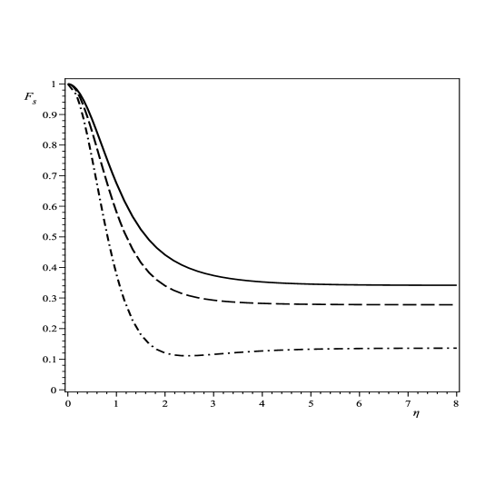
Figure 2: $F_{s}$ versus $\eta$ in the W case plotted for $\gamma=20$, for the boosts along the $z$-axis. The solid curve is plotted for the momentum product (zero momentum entanglement) while the dashed curve and the dashed-dotted curve correspond to the 2-momentum correlated and 3-momentum correlated cases, respectively.

5 Conclusions

In this work we investigated a system of three massive particles described by a Gaussian momentum distributed wave packet such that in the rest frame its spin part was entangled as the GHZ state or the W state. Then we constructed the wave packet of the system as viewed by a boosted observer, by using the corresponding Wigner rotation operators. We focused on the spin part of the system by tracing out the momentum part and finding the reduced density operators both for the rest observer and the boosted observer. Using these reduced density matrices and the Uhlmann formula for fidelity, the spin fidelities were formulated separately when there was no momentum correlation, when two of three momenta were correlated and when all the three momenta were correlated. We could not evaluate fidelities analytically, so we utilized a numerical approach to plot $F_{s}$ in terms of the boost parameter $\eta$, as Fig.s 1 and 2 show.

We conclude that for the GHZ case, by increasing the boost velocity, $F_{s}$ falls to non-zero asymptotic values that increase as the momenta become more entangled. One may explain this behavior by regarding the results of the refs. [3] and [4]. By boosting the wave packet, we move some of the spin entanglement to the momentum part and simultaneously the momentum entanglement appears to to be moved to the spins. The amount of transferred entanglement grows with increasing the boost velocity. Tracing out the momentum from the Lorentz-transformed density matrix destroys some of the entanglement. This process causes to decrease the spin entanglement in the boosted frame. When the momenta are correlated, the transfer of momentum entanglement to spins compensates somewhat the decrease of spin entanglement and then the spin fidelity decreases less. However, as the figures show, this becomes more significant at large boost velocities. For the W case, the situation is inverse and by increasing the momentum entanglement, the spin fidelity decreases more.

References

[1]
A. Peres, P. F. Scudo, and D. R. Terno.
Phys. Rev. Lett., 88:230402, 2002.
[2]
P. M. Alsing and G. J. Milborn.
Quantum Inf. Comput., 2:487, 2002.
[3]
R. M. Gingrich and C. Adami.
Phys. Rev. Lett., 89:270402, 2002.
[4]
H. Li and J. Du.
Phys. Rev. A, 68:022108, 2003.
[5]
S. D. Bartlett and D. R. Terno.
Phys. Rev. A, 71:012302, 2005.
[6]
F. Jordan, A. Shaji, and E. C. G. Sudarshan.
Phys. Rev. A, 75:022101, 2007.
[7]
B. Nasr Esfahani, F. Ahmadi, and M. Ahmadi.
Int. J. Theor. Phys, 48:1957–1964, 2009.
[8]
M. Czachor.
Phys. Rev. A, 55:77, 1997.
[9]
D. Ahn, H. J. Lee, Y. H. Moon, and S. W. Hwang.
Phys. Rev. A, 67:012103, 2003.
[10]
D. Lee and C. Y. Ee.
New J. Phys., 6:67, 2004.
[11]
Y. H. Moon, S. W. Hwang, and D. Ahn.
Prog. Theor. Phys., 112:219, 2004.
[12]
W. T. Kim and E. J. Son.
Phys. Rev. A, 71:0141107, 2005.
[13]
H. Terashima and M. Ueda.
Quantum Inf. Comput., 3:224, 2003.
[14]
S. Moradi.
Phys. Rev. A, 77:024101, 2008.
[15]
M. A. Horne D. M. Greenberger and A. Zeilinger.
Bell s Theorem, Quantum Theory, and Conceptions of the
Universe.
Kluwer, Dordrecht, 1989.
[16]
D. M. Greenberger, M. A. Horne, A. Shimony, and A.Zeilinger.
Am. J. Phys, 58:1131, 1990.
[17]
P. Agarwal and A. K. Pati.
Phys. Rev. A, 74:1131, 1990.
[18]
W. Dr, G. Vidal, and J. I. Cirac.
Phys. Rev. A, 62:062314, 2000.
[19]
D. Bouwmeester, Jian-Wei Pan, M. Danielland H. Weinfurter, and
A. Zeilinger.
Phys. Rev. Lett., 82:1345, 1999.
[20]
H. Jeong and N. B. An.
Phys. Rev. A, 74:022104, 2006.
[21]
J. Wen and M. H. Rubin.
Phys. Rev. A, 79:025802, 2009.
[22]
S. S. Sharma.
Phys. Lett. A, 311:111–114, 2003.
[23]
L. Jin and Z. Song.
Phys. Rev. A, 79:042341, 2009.
[24]
S. Weinberg.
The Quantum Theory of Fields.
Cambridge University press, Cambridge, 1995.
[25]
A. Uhlman.
Rep. Math. Phys., 9:273–279, 1976.
[26]
M. Hubner.
Phys. Lett. A, 179:226–230, 1993.
[27]
T. C. Wei and P. M. Goldbart.
Phys. Rev. A, 68:042307, 2003.
[28]
L. Lamata, J. Le n, and E. Solano.
Phys. Rev. A, 73:012335, 2006.