Anisotropic Power-law Inflation

Abstract

We study an inflationary scenario in supergravity model with a gauge kinetic function. We find exact anisotropic power-law inflationary solutions when both the potential function for an inflaton and the gauge kinetic function are exponential type. The dynamical system analysis tells us that the anisotropic power-law inflation is an attractor for a large parameter region.

I Introduction

It is believed that inflationary scenario explains main features of cosmic microwave background radiation (CMB) observed by WMAP Komatsu:2010fb . The remarkable predictive power of inflation is associated with the cosmic no-hair conjecture which claims that any classical hair will disappear exponentially fast once the vacuum energy dominates the universe. As a result, there remain quantum vacuum fluctuations which become seeds of the large scale structure of the universe. The quantum vacuum fluctuations give rise to the following robust predictions. The power spectrum of fluctuations should have the statistical isotropy due to the symmetry of deSitter background. The scale dependence of power spectrum should be absent because of the time translation invariance of deSitter spacetime. The slow roll conditions should suppress nonlinearity and hence yield Gaussian statistics of fluctuations. These predictions have been observationary proved in rough.

Nowadays, however, precise cosmological observations force us to look at fine structures of an inflationary universe. Actually, the inflationary universe is not exactly deSitter and deviation from the exact deSitter is characterized by slow roll parameters of the order of a few percent. Indeed, the deviation from the scale free spectrum is well known. Moreover, it has been shown that the deviation from Gaussianity in a single inflaton model is determined by the slow roll parameters Maldacena:2002vr . From these examples of deviations, it would be quite natural to expect statistical anisotropy of the order of the slow roll parameter Yokoyama:2008xw ; Dimopoulos:2009vu ; ValenzuelaToledo:2009af ; ValenzuelaToledo:2009nq ; Dimastrogiovanni:2010sm ; BlancoPillado:2010uw ; Adamek:2010sg . However, a prejudice due to the cosmic no-hair conjecture has prevented us seeking the statistical anisotropy seriously.

Historically, there have been challenges to the cosmic no-hair conjecture Ford:1989me ; Kaloper:1991rw ; Barrow:2005qv ; Barrow:2009gx ; Campanelli:2009tk ; Golovnev:2008cf ; Kanno:2008gn ; Ackerman:2007nb . Unfortunately, it turned out that these models suffer from either the instability Himmetoglu:2008zp ; Golovnev:2009rm ; EspositoFarese:2009aj , or a fine tuning problem, or a naturalness problem. Recently, however, we have succeeded in finding stable anisotropic inflationary solutions in a natural set-up, which provide counter examples to the cosmic no-hair conjecture Watanabe:2009ct ; Kanno:2009ei . More precisely, we have shown that, in the presence of a vector field coupled with the inflaton, there could be a small anisotropy in the expansion rate which never decays during inflation. Furthermore, since the anisotropic inflation is an attractor solution, the predictive power of the model still remains Himmetoglu:2009mk ; Dulaney:2010sq ; Gumrukcuoglu:2010yc ; Watanabe:2010fh . The imprints of the anisotropic expansion could be found in the fine structures of the CMB Watanabe:2010bu .

Our anisotropic inflationary model is motivated by supergravity which can be regarded as a low energy limit of superstring theory. It is well known that the supergravity models can be constrained by comparing predictions of inflation with cosmological observations. For example, the tilt of the spectrum gives interesting information of the superpotential $W(\phi^{i})$ and the Kaler potential $K(\phi^{i},\bar{\phi}^{i})$ which are functionals of complex scalar fields. Here, a bar represents a complex conjugate. The information will provide a hint to the fundamental theory. More concretely, the bosonic part of the action of supergravity reads

$$S=\int d^{4}x\sqrt{-g}\left[\frac{1}{2\kappa^{2}}R+K_{i\bar{j}}\partial^{\mu}\phi^{i}\partial_{\mu}\bar{\phi}^{\bar{j}}-e^{K}K^{i\bar{j}}D_{i}WD_{\bar{j}}\bar{W}-f_{ab}(\phi)F^{a}_{\mu\nu}F^{b\mu\nu}\right]$$ (1)

where we have defined $K_{i\bar{j}}=\partial^{2}K/\partial\phi^{i}\partial\bar{\phi}^{j}$ and $D_{i}W=\partial W/\partial\phi^{i}+\partial K/\partial\phi^{i}W$. Here, we note that the gauge kinetic function $f_{ab}(\phi)$ in front of the vector kinetic term $F^{a}_{\mu\nu}F^{b\mu\nu}$ could be nontrivial functions of the scalar fields. Interestingly, so far, the vector part has been neglected in most of discussion of inflation. The reason is partially due to the cosmic no-hair conjecture which states that the anisotropy, curvature, and any matter will vanish once the inflation commences. As we mentioned, however this is not true when we look at percent level fine structures of inflationary scenarios.

From the point of view of precision cosmology, it is important to explore the role of the gauge kinetic function in inflation. In the previous work, we have used rather unconventional functional form $\propto\exp(c\phi^{2})$ (c is a constant) for the gauge kinetic function Martin:2007ue . Although we have also mentioned general cases, it is desirable to investigate more natural cases explicitly. It is well known that the exponential type functional form is ubiquitous from the point of view of dimensional reduction of higher dimensional theory. Hence, in this paper, we study the cases where a functional form for the potential and the gauge kinetic function is an exponential dependence on the inflaton. In particular, we present exact anisotropic inflationary solutions. Moreover, we demonstrate these solutions become attractors for a large parameter region.

The organization of the paper is as follows. In section II, we introduce inflationary models where the vector field couples with an inflaton and obtain exact solutions which contain anisotropic power-law solutions. In section III, we investigate solution space with dynamical system approach and show that the anisotropic inflation is an attractor for a large parameter region. The final section is devoted to the conclusion.

II Exact Anisotropic Inflationary Solutions

In this section, we consider a simple model with exponential potential and gauge kinetic functions and then find exact power-law solutions. In addition to a well known isotropic power-law solution, we find an anisotropic power-law inflation.

We consider the following action for the gravitational field, the inflaton field $\phi$ and the vector field $A_{\mu}$ coupled with $\phi$:

$$S=\int d^{4}x\sqrt{-g}\left[~{}\frac{M_{p}^{2}}{2}R-\frac{1}{2}\left(\partial_{\mu}\phi\right)\left(\partial^{\mu}\phi\right)-V(\phi)-\frac{1}{4}f^{2}(\phi)F_{\mu\nu}F^{\mu\nu}~{}\right]\ ,$$ (2)

where $g$ is the determinant of the metric, $R$ is the Ricci scalar, respectively. Here, $M_{p}$ represents the reduced Planck mass. The field strength of the vector field is defined by $F_{\mu\nu}=\partial_{\mu}A_{\nu}-\partial_{\nu}A_{\mu}$. Motivated by the dimensional reduction of higher dimensional theory such as string theory, we assume the exponential potential

$$V(\phi)=V_{0}e^{\lambda\frac{\phi}{M_{p}}}$$ (3)

and the exponential gauge kinetic function

$$f(\phi)=f_{0}e^{\rho\frac{\phi}{M_{p}}}\ .$$ (4)

In principle, the parameters $V_{0},f_{0},\lambda$, and $\rho$ can be determined once the compactification scheme is specified. However, we leave those free in this paper.

Using the gauge invariance, we can choose the gauge $A_{0}=0$. Without loosing the generality, we can take the $x$-axis in the direction of the vector field. Hence, we have the homogeneous fields of the form $A_{\mu}=(~{}0,~{}v(t),~{}0,~{}0~{})$ and $\phi=\phi(t)\ .$ As there exists the rotational symmetry in the $y$-$z$ plane now, we take the metric to be

$$ds^{2}=-dt^{2}+e^{2\alpha(t)}\left[~{}e^{-4\sigma(t)}dx^{2}+e^{2\sigma(t)}\left(dy^{2}+dz^{2}\right)~{}\right]\ ,$$ (5)

where the cosmic time $t$ is used. Here, $e^{\alpha}$ is an isotropic scale factor and $\sigma$ represents a deviation from the isotropy. With above ansatz, the equations of motion can be written down as

$$\dot{\alpha}^{2}=\dot{\sigma}^{2}+\frac{1}{3M_{p}^{2}}\left[\frac{1}{2}\dot{\phi}^{2}+V(\phi)+\frac{1}{2}f^{2}(\phi)e^{-2\alpha+4\sigma}\dot{v}^{2}\right]\ ,$$ (6)

$$\ddot{\alpha}=-3\dot{\alpha}^{2}+\frac{1}{M_{p}^{2}}V(\phi)+\frac{1}{6M_{p}^{2}}f^{2}(\phi)e^{-2\alpha+4\sigma}\dot{v}^{2}\ ,$$ (7)

$$\ddot{\sigma}=-3\dot{\alpha}\dot{\sigma}+\frac{1}{3M_{p}^{2}}f^{2}(\phi)e^{-2\alpha+4\sigma}\dot{v}^{2},$$ (8)

$$\ddot{\phi}=-3\dot{\alpha}\dot{\phi}-V^{\prime}(\phi)+f(\phi)f^{\prime}(\phi)e^{-2\alpha+4\sigma}\dot{v}^{2}\ ,$$ (9)

$$\frac{d}{dt}\left[f^{2}e^{\alpha+4\sigma}\dot{v}\right]=0\ ,$$ (10)

where an overdot and a prime denote the derivative with respect to the cosmic time $t$ and $\phi$, respectively. We find Eq. (10) can be easily solved as

$$\dot{v}=f^{-2}(\phi)e^{-\alpha-4\sigma}p_{A},$$ (11)

where $p_{A}$ denotes a constant of integration. Substituting (11) into other equations, we obtain equations

$$\dot{\alpha}^{2} = \dot{\sigma}^{2}+\frac{1}{3M_{p}^{2}}\left[\frac{1}{2}\dot{\phi}^{2}+V(\phi)+\frac{p_{A}^{2}}{2}f^{-2}(\phi)e^{-4\alpha-4\sigma}\right]\ ,$$ (12)

$$\ddot{\alpha} = -3\dot{\alpha}^{2}+\frac{1}{M_{p}^{2}}V(\phi)+\frac{p_{A}^{2}}{6M_{p}^{2}}f^{-2}(\phi)e^{-4\alpha-4\sigma},$$ (13)

$$\ddot{\sigma} = -3\dot{\alpha}\dot{\sigma}+\frac{p_{A}^{2}}{3M_{p}^{2}}f^{-2}(\phi)e^{-4\alpha-4\sigma},$$ (14)

$$\ddot{\phi} = -3\dot{\alpha}\dot{\phi}-V^{\prime}(\phi)+p_{A}^{2}f^{-3}(\phi)f^{\prime}(\phi)e^{-4\alpha-4\sigma}\ .$$ (15)

In the case of no vector fields, there exists the power-law inflationary solution Abbott:1984fp ; Lucchin:1984yf ; Barrow:1987ia ; Halliwell:1986ja ; Burd:1988ss . Therefore, let us first seek the power-law solutions by assuming

$$\alpha=\zeta\log t\ ,\hskip 28.45274pt\sigma=\eta\log t\ ,\hskip 28.45274pt\frac{\phi}{M_{p}}=\xi\log t+\phi_{0}\ .$$ (16)

Apparently, for a trivial vector field $p_{A}=0$, we have the isotropic power-law solution

$$\zeta=\frac{2}{\lambda^{2}}\ ,\hskip 28.45274pt\eta=0\ ,\hskip 28.45274pt\xi=-\frac{2}{\lambda}\ ,\hskip 28.45274pt\frac{V_{0}}{M^{2}_{p}}e^{\lambda\phi_{0}}=\frac{2(6-\lambda^{2})}{\lambda^{4}}\ .$$ (17)

In this case, we have the spacetime

$$ds^{2}=-dt^{2}+t^{4/\lambda^{2}}\left(dx^{2}+dy^{2}+dz^{2}\right)\ .$$ (18)

Hence, we need $\lambda\ll 1$ for obtaining the sufficiently fast expansion.

Next, interestingly, we see that there exists the other non-trivial exact solution in spite of the existence of the no-hair theorem  Wald:1983ky ; Kitada:1991ih ; Kitada:1992uh . From the hamiltonian constraint equation (12), we set two relations

$$\lambda\xi=-2\ ,\hskip 28.45274pt\rho\xi+2\zeta+2\eta=1$$ (19)

to have the same time dependence for each term. The latter relation is necessary only in the non-trivial vector case, $p_{A}\neq 0$. Then, for the amplitudes to balance, we need

$$-\zeta^{2}+\eta^{2}+\frac{1}{6}\xi^{2}+\frac{1}{3}u+\frac{1}{6}w=0\ ,$$ (20)

where we have defined

$$u=\frac{V_{0}}{M_{p}^{2}}e^{\lambda\phi_{0}}\ ,\hskip 28.45274ptw=\frac{p_{A}^{2}}{M_{p}^{2}}f_{0}^{-2}e^{-2\rho\phi_{0}}\,.$$ (21)

The equation for the scale factor (13) under Eq. (19) yields

$$-\zeta+3\zeta^{2}-u-\frac{1}{6}w=0\ .$$ (22)

Similarly, the equation for the anisotropy (14) gives

$$-\eta+3\zeta\eta-\frac{1}{3}w=0\ .$$ (23)

Finally, from the equation for the scalar (15), we obtain

$$-\xi+3\zeta\xi+\lambda u-\rho w=0\ .$$ (24)

Using Eqs. (19), (22) and (23), we can solve $u$ and $w$ as

$$u=\frac{9}{2}\zeta^{2}-\frac{9}{4}\zeta-\frac{3\rho}{2\lambda}\zeta+\frac{1}{4}+\frac{\rho}{2\lambda}\ ,\hskip 28.45274ptw=-9\zeta^{2}+\frac{15}{2}\zeta+\frac{9\rho}{\lambda}\zeta-\frac{3}{2}-\frac{3\rho}{\lambda}\,.$$ (25)

Substituting these results into Eq. (24), we obtain

$$\left(3\zeta-1\right)\left[6\lambda\left(\lambda+2\rho\right)\zeta-\left(\lambda^{2}+8\rho\lambda+12\rho^{2}+8\right)\right]=0\ .$$ (26)

In the case of $\zeta=1/3$, we have $u=w=0$. Hence, it is not our desired solution. Thus, we have to choose

$$\zeta=\frac{\lambda^{2}+8\rho\lambda+12\rho^{2}+8}{6\lambda(\lambda+2\rho)}\ .$$ (27)

Substituting this result into Eq. (22), we obtain

$$\eta=\frac{\lambda^{2}+2\rho\lambda-4}{3\lambda(\lambda+2\rho)}\,.$$ (28)

From Eq. (19), we have

$$\xi=-\frac{2}{\lambda}\,.$$ (29)

Finally, Eq. (25) reduce to

$$u=\frac{(\rho\lambda+2\rho^{2}+2)(-\lambda^{2}+4\rho\lambda+12\rho^{2}+8)}{2\lambda^{2}(\lambda+2\rho)^{2}}$$ (30)

and

$$w=\frac{(\lambda^{2}+2\rho\lambda-4)(-\lambda^{2}+4\rho\lambda+12\rho^{2}+8)}{2\lambda^{2}(\lambda+2\rho)^{2}}\ .$$ (31)

Note that Eq. (20) is automatically satisfied.

In order to have inflation, we need $\lambda\ll 1$. For these cases, $u$ is always positive. Since $w$ should be also positive, we have the condition

$$\lambda^{2}+2\rho\lambda>4\ .$$ (32)

Hence, $\rho$ must be much larger than one. Now, the spacetime reads

$$ds^{2}=-dt^{2}+t^{2\zeta-4\eta}dx^{2}+t^{2\zeta+2\eta}\left(dy^{2}+dz^{2}\right)\ .$$ (33)

The average expansion rate is determined by $\zeta$ and the average slow roll parameter is given by

$$\epsilon\equiv-\frac{\dot{H}}{H^{2}}=\frac{6\lambda(\lambda+2\rho)}{\lambda^{2}+8\rho\lambda+12\rho^{2}+8}\ ,$$ (34)

where we have defined $H=\dot{\alpha}$. In the limit $\lambda\ll 1$ and $\rho\gg 1$, this reduces to $\epsilon=\lambda/\rho$. Now, the anisotropy is characterized by

$$\frac{\Sigma}{H}\equiv\frac{\dot{\sigma}}{\dot{\alpha}}=\frac{2(\lambda^{2}+2\rho\lambda-4)}{\lambda^{2}+8\rho\lambda+12\rho^{2}+8}\ .$$ (35)

From Eq. (34) and (35), we obtain a relation

$$\frac{\Sigma}{H}=\frac{1}{3}I\epsilon\,,\hskip 28.45274ptI=\frac{\lambda^{2}+2\rho\lambda-4}{\lambda^{2}+2\rho\lambda}\,.$$ (36)

In order to see the relation to our previous result  Watanabe:2009ct ; Watanabe:2010fh , we can rewrite the above result as

$$I=\frac{c-1}{c}\,,\hskip 28.45274ptc=\frac{\lambda^{2}+2\rho\lambda}{4}\ .$$ (37)

Thus, the result is consistent with our previous analysis.

Although the anisotropy is always small, it persists during inflation. Clearly these exact solutions give rise to counter examples to the cosmic no-hair conjecture. We should note that the cosmological constant is assumed in the cosmic no-hair theorem presented by Wald Wald:1983ky . In the case of isolated vacuum energy, the inflaton can mimic the cosmological constant  Kitada:1991ih ; Kitada:1992uh ; Aguirregabiria:1993pm . However, in the presence of the non-trivial coupling between the inflaton and the vector field, the cosmic no-hair theorem cannot be applicable anymore.

III Stability of Anisotropic Inflation

In the previous section, we found isotropic and anisotropic power-law solutions. In this section, we will investigate the phase space structure. Then, we will see which one is dynamically selected.

Let us use e-folding number as a time coordinate $d\alpha=\dot{\alpha}dt$. It is convenient to define dimensionless variables

$$X=\frac{\dot{\sigma}}{\dot{\alpha}}\ ,\hskip 28.45274ptY=\frac{1}{M_{p}}\frac{\dot{\phi}}{\dot{\alpha}}\ ,\hskip 28.45274ptZ=\frac{f(\phi)}{M_{p}}e^{-\alpha+2\sigma}\frac{\dot{v}}{\dot{\alpha}}\ .$$ (38)

With these definitions, we can write the hamiltonian constraint equation as

$$-\frac{1}{M_{p}^{2}}\frac{V}{\dot{\alpha}^{2}}=3(X^{2}-1)+\frac{1}{2}Y^{2}+\frac{1}{2}Z^{2}\ .$$ (39)

Since we are considering a positive potential, we have the inequality

$$3(X^{2}-1)+\frac{1}{2}Y^{2}+\frac{1}{2}Z^{2}<0\ .$$ (40)

Using the hamiltonian constraint (39), we can eliminate $\phi$ from the equations of motion. Thus, the equations of motion can be reduced to the autonomous form:

$$\frac{dX}{d\alpha} = \frac{1}{3}Z^{2}(X+1)+X\left\{3(X^{2}-1)+\frac{1}{2}Y^{2}\right\}\,,$$ (41)

$$\frac{dY}{d\alpha} = (Y+\lambda)\left\{3(X^{2}-1)+\frac{1}{2}Y^{2}\right\}+\frac{1}{3}YZ^{2}+\left(\rho+\frac{\lambda}{2}\right)Z^{2}\,,$$ (42)

$$\frac{dZ}{d\alpha} = Z\left[3(X^{2}-1)+\frac{1}{2}Y^{2}-\rho Y+1-2X+\frac{1}{3}Z^{2}\right]\ .$$ (43)

Therefore, we have 3-dimensional space with a constraint (40) and the fixed point is defined by $dX/d\alpha=dY/d\alpha=dZ/d\alpha=0$.

First, we seek the isotropic fixed point $X=0$. From Eq. (41), we see $Z=0$. The remaining equation (42) yields $Y=-\lambda$ or $Y^{2}=6$. The latter solution does not satisfy the constraint (40). Thus, the isotropic fixed point becomes

$$(X,Y,Z)=(0,-\lambda,0)\ .$$ (44)

This fixed point corresponds to the isotropic power-law solution (18). Indeed, one can check the solution (17) leads to the above fixed point.

Apparently, $Z=0$ and $6X^{2}+Y^{2}=6$ give a fixed curve. However, this contradicts the constraint (40).

Now, let us find an anisotropic fixed point. From Eqs. (41) and (42), we have

$$Y=\left(3\rho+\frac{\lambda}{2}\right)X-\lambda\ .$$ (45)

Eq. (41) gives

$$Z^{2}=-\frac{3X}{X+1}\left[3(X^{2}-1)+\frac{1}{2}Y^{2}\right]\ .$$ (46)

Using the above results in Eq. (43), we have

$$\left(X-2\right)\left[\left(\lambda^{2}+8\rho\lambda+12\rho^{2}+8\right)X-2\left(\lambda^{2}+2\rho\lambda-4\right)\right]=0\ .$$ (47)

The solution $X=2$ does not make sense because it implies $Z^{2}=-18-36\rho^{2}<0$ by Eqs. (45) and (46). Thus, an anisotropic fixed point is expressed by

$$X=\frac{2\left(\lambda^{2}+2\rho\lambda-4\right)}{\lambda^{2}+8\rho\lambda+12\rho^{2}+8}\ .$$ (48)

Substituting this result into Eq. (45), we obtain

$$Y=-\frac{12\left(\lambda+2\rho\right)}{\lambda^{2}+8\rho\lambda+12\rho^{2}+8}\ .$$ (49)

Eq. (46) yields

$$Z^{2}=\frac{18\left(\lambda^{2}+2\rho\lambda-4\right)\left(-\lambda^{2}+4\rho\lambda+12\rho^{2}+8\right)}{\left(\lambda^{2}+8\rho\lambda+12\rho^{2}+8\right)^{2}}\ .$$ (50)

Note that from the last equation, we find $\lambda^{2}+2\rho\lambda>4$ is required for this fixed point to exist under inflation $\lambda\ll 1$. It is not difficult to confirm that this fixed point corresponds to the anisotropic power-law solution (33).

Next, we examine the linear stability of fixed points. The linearized equations for Eqs. (41), (42), (43) are given by

$$\frac{d\delta X}{d\alpha} = \left(\frac{1}{3}Z^{2}+9X^{2}+\frac{1}{2}Y^{2}-3\right)\delta X+XY\delta Y+\frac{2}{3}\left(X+1\right)Z\delta Z\,,$$ (51)

$$\frac{d\delta Y}{d\alpha} = 6X\left(Y+\lambda\right)\delta X\,,$$ (52)

$$+\left\{3\left(X^{2}-1\right)+\frac{1}{2}Y^{2}+Y\left(Y+\lambda\right)+\frac{1}{3}Z^{2}\right\}\delta Y+\left(\frac{2}{3}Y+2\rho+\lambda\right)Z\delta Z\,,$$

$$\frac{d\delta Z}{d\alpha} = 2(3X-1)Z\delta X+\left(Y-\rho\right)Z\delta Y+\left(3X^{2}+\frac{1}{2}Y^{2}+Z^{2}-2X-\rho Y-2\right)\delta Z\,.$$ (53)

In the case of the isotropic fixed point Eq. (44), these equations reduce to

$$\frac{d\delta X}{d\alpha} = \left(\frac{1}{2}\lambda^{2}-3\right)\delta X\,,$$ (54)

$$\frac{d\delta Y}{d\alpha} = \left(\frac{1}{2}\lambda^{2}-3\right)\delta Y\,,$$ (55)

$$\frac{d\delta Z}{d\alpha} = \left[\frac{1}{2}\lambda^{2}-2+\rho\lambda\right]\delta Z\,.$$ (56)

We see that the left hand side of all above equations becomes negative when $\lambda^{2}+2\rho\lambda<4$ during inflation $\lambda\ll 1$, which means the isotropic fixed point is an attractor under these conditions and the isotropic fixed point becomes stable in this parameter region. In the opposite case, $\lambda^{2}+2\rho\lambda>4$, the fixed point becomes a saddle point and unstable.

Now we are interested in the fate of trajectories around the unstable isotropic fixed point. We will see that those trajectories converge to an anisotropic fixed point.

Since we are considering the inflationary universe $\lambda\ll 1$, the condition $\lambda^{2}+2\rho\lambda>4$ implies $\rho\gg 1$. Under these conditions, we can approximately write down the linear equations as

$$\frac{d\delta X}{d\alpha} = -3\delta X\,,$$ (57)

$$\frac{d\delta Y}{d\alpha} = -3\delta Y+\sqrt{6(\lambda^{2}+2\rho\lambda-4)}\delta Z\,,$$ (58)

$$\frac{d\delta Z}{d\alpha} = -\frac{1}{2}\sqrt{6(\lambda^{2}+2\rho\lambda-4)}\delta Y\ .$$ (59)

The stability can be analyzed by setting

$$\delta X=e^{\omega\alpha}\delta\tilde{X}\ ,\hskip 28.45274pt\delta Y=e^{\omega\alpha}\delta\tilde{Y}\ ,\hskip 28.45274pt\delta Z=e^{\omega\alpha}\delta\tilde{Z}\ .$$ (60)

Then we find the eigenvalues $\omega$ are given by

$$\omega=-3\ ,-\frac{3}{2}\pm i\sqrt{3(\lambda^{2}+2\rho\lambda-4)-\frac{9}{4}}\ .$$ (61)

As the eigenvalues have negative real part, the anisotropic fixed point is stable. Thus, the end point of trajectories around the unstable isotropic power-law inflation must be the anisotropic power-law inflation.

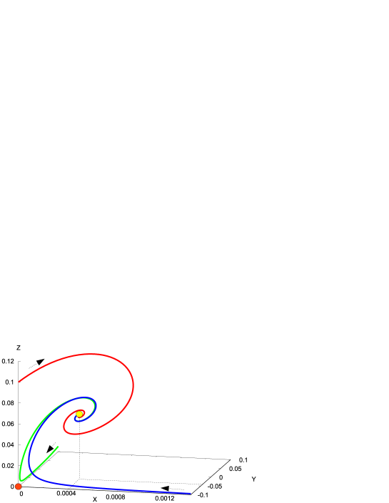
Figure 1: The phase flow in $X$-$Y$-$Z$ space is depicted for $\lambda=0.1,\rho=50$. The yellow and orange circles indicate the anisotropic and isotropic fixed points respectively. The trajectories converge to the anisotropic fixed point.

In Fig.1, we depicted the phase flow in $X$-$Y$-$Z$ space for $\lambda=0.1,\ \rho=50$. We see that the trajectories converge to the anisotropic fixed point indicated by yellow circle. The isotropic fixed point indicated by orange circle is a saddle point which is an attractor only on $Z=0$ plane. Thus, the anisotropic power-law inflation is an attractor solution for parameters satisfying $\lambda^{2}+2\rho\lambda>4$.

IV Conclusion

We have examined a supergravity model with a gauge kinetic function. It turned out that exact anisotropic power-law inflationary solutions exist when both the potential function for an inflaton and the gauge kinetic function are exponential type. We showed that the degree of the anisotropy is proportional to the slow roll parameter. The slow roll parameter depends both on the potential function and the gauge kinetic function. The dynamical system analysis proved that the anisotropic power-law inflation is an attractor for a large parameter region $\lambda^{2}+2\rho\lambda>4$. Therefore, the result we have found in this paper indicates that the cosmic no-hair conjecture should be modified appropriately.

The imprint of the geometrical symmetry breakdown during inflation can be found in the cosmic microwave background radiation. We should note that the statistical anisotropy could be large even when the anisotropy in the expansion is quite small Dulaney:2010sq ; Gumrukcuoglu:2010yc ; Watanabe:2010fh .

The result in this paper also has implication in cosmological magnetic fields Kanno:2009ei ; Moniz:2010cm . In the original paper by Ratra, the same potential and gauge kinetic functions are assumed Ratra:1991bn ; Ratra:1991av . Hence, it is interesting to incorporate backreaction into his analysis.

Note added: Recently, anisotropic inflationary scenarios with other potential functions have been investigated in Hassan . In their paper, a charged scalar field plays an important role and induces an interesting behavior around the reheating stage. We thank the authors for a preview of their paper which is complementary to our work.

- (1) E. Komatsu et al., arXiv:1001.4538 [astro-ph.CO].
- (2) J. M. Maldacena, JHEP 0305, 013 (2003).
- (3) S. Yokoyama and J. Soda, JCAP 0808, 005 (2008) [arXiv:0805.4265 [astro-ph]].
- (4) K. Dimopoulos, M. Karciauskas, D. H. Lyth and Y. Rodriguez, JCAP 0905, 013 (2009) [arXiv:0809.1055 [astro-ph]]; K. Dimopoulos, M. Karciauskas and J. M. Wagstaff, Phys. Lett. B 683, 298 (2010) [arXiv:0909.0475 [hep-ph]].
- (5) C. A. Valenzuela-Toledo, Y. Rodriguez and D. H. Lyth, Phys. Rev. D 80, 103519 (2009) [arXiv:0909.4064 [astro-ph.CO]].
- (6) C. A. Valenzuela-Toledo and Y. Rodriguez, Phys. Lett. B 685, 120 (2010) [arXiv:0910.4208 [astro-ph.CO]].
- (7) E. Dimastrogiovanni, N. Bartolo, S. Matarrese and A. Riotto, arXiv:1001.4049 [astro-ph.CO].
- (8) J. J. Blanco-Pillado and M. P. Salem, JCAP 1007, 007 (2010) [arXiv:1003.0663 [hep-th]].
- (9) J. Adamek, D. Campo and J. C. Niemeyer, Phys. Rev. D 82, 086006 (2010) [arXiv:1003.3204 [hep-th]].
- (10) L. H. Ford, Phys. Rev. D 40, 967 (1989).
- (11) N. Kaloper, Phys. Rev. D 44, 2380 (1991).
- (12) J. D. Barrow and S. Hervik, Phys. Rev. D 73, 023007 (2006) [arXiv:gr-qc/0511127].
- (13) J. D. Barrow and S. Hervik, Phys. Rev. D 81, 023513 (2010) [arXiv:0911.3805 [gr-qc]].
- (14) L. Campanelli, Phys. Rev. D 80, 063006 (2009) [arXiv:0907.3703 [astro-ph.CO]].
- (15) A. Golovnev, V. Mukhanov and V. Vanchurin, JCAP 0806, 009 (2008) [arXiv:0802.2068 [astro-ph]];
- (16) S. Kanno, M. Kimura, J. Soda and S. Yokoyama, JCAP 0808, 034 (2008).
- (17) L. Ackerman, S. M. Carroll and M. B. Wise, Phys. Rev. D 75, 083502 (2007).
- (18) B. Himmetoglu, C. R. Contaldi and M. Peloso, arXiv:0809.2779 [astro-ph]; B. Himmetoglu, C. R. Contaldi and M. Peloso, arXiv:0812.1231 [astro-ph]; B. Himmetoglu, C. R. Contaldi and M. Peloso, Phys. Rev. D 80, 123530 (2009) [arXiv:0909.3524 [astro-ph.CO]].
- (19) A. Golovnev, Phys. Rev. D 81, 023514 (2010) [arXiv:0910.0173 [astro-ph.CO]].
- (20) G. Esposito-Farese, C. Pitrou and J. P. Uzan, Phys. Rev. D 81, 063519 (2010) [arXiv:0912.0481 [gr-qc]].
- (21) M. a. Watanabe, S. Kanno and J. Soda, Phys. Rev. Lett. 102, 191302 (2009) [arXiv:0902.2833 [hep-th]].
- (22) S. Kanno, J. Soda and M. a. Watanabe, JCAP 0912, 009 (2009) [arXiv:0908.3509 [astro-ph.CO]].
- (23) B. Himmetoglu, arXiv:0910.3235 [astro-ph.CO].
- (24) T. R. Dulaney and M. I. Gresham, arXiv:1001.2301 [astro-ph.CO].
- (25) A. E. Gumrukcuoglu, B. Himmetoglu and M. Peloso, arXiv:1001.4088 [astro-ph.CO].
- (26) M. a. Watanabe, S. Kanno and J. Soda, Prog. Theor. Phys. 123, 1041 (2010) [arXiv:1003.0056 [astro-ph.CO]].
- (27) M. a. Watanabe, S. Kanno and J. Soda, arXiv:1011.3604 [astro-ph.CO].
- (28) J. Martin and J. Yokoyama, JCAP 0801, 025 (2008).
- (29) L. F. Abbott and M. B. Wise, Nucl. Phys. B 244, 541 (1984).
- (30) F. Lucchin and S. Matarrese, Phys. Rev. D 32, 1316 (1985).
- (31) J. D. Barrow, Phys. Lett. B 187, 12 (1987).
- (32) J. J. Halliwell, Phys. Lett. B 185, 341 (1987).
- (33) A. B. Burd and J. D. Barrow, Nucl. Phys. B 308, 929 (1988).
- (34) R. M. Wald, Phys. Rev. D 28, 2118 (1983).
- (35) Y. Kitada and K. i. Maeda, Phys. Rev. D 45, 1416 (1992).
- (36) Y. Kitada and K. i. Maeda, Class. Quant. Grav. 10, 703 (1993).
- (37) J. M. Aguirregabiria, A. Feinstein and J. Ibanez, Phys. Rev. D 48, 4662 (1993) [arXiv:gr-qc/9309013].
- (38) B. Ratra, Astrophys. J. 391, L1 (1992).
- (39) B. Ratra, “Inflation generated cosmological magnetic field,” 1991.
- (40) P. V. Moniz and J. Ward, arXiv:1007.3299 [gr-qc].
- (41) R. Emami, H. Firouzjahi, S. M. S. Movahed and M. Zarei, arXiv:1010.5495 [astro-ph.CO].