Thermodynamic Geometry:
Evolution, Correlation and Phase Transition

Abstract

Under the fluctuation of the electric charge and atomic mass, this paper considers the theory of the thin film depletion layer formation of an ensemble of finitely excited, non-empty $d/f$-orbital heavy materials, from the thermodynamic geometric perspective. At each state of the local adiabatic evolutions, we examine the nature of the thermodynamic parameters, viz., electric charge and mass, changing at each respective embeddings. The definition of the intrinsic Riemannian geometry and differential topology offers the properties of (i) local heat capacities, (ii) global stability criterion and (iv) global correlation length. Under the Gaussian fluctuations, such an intrinsic geometric consideration is anticipated to be useful in the statistical coating of the thin film layer of a desired quality-fine high cost material on a low cost durable coatant. From the perspective of the daily-life applications, the thermodynamic geometry is thus intrinsically self-consistent with the theory of the local and global economic optimizations. Following the above procedure, the quality of the thin layer depletion could self-consistently be examined to produce an economic, quality products at a desired economic value.

Keywords: Thermodynamic Geometry, Metal Depletion, Nano-science, Thin Film Technology, Quality Economic Characterization

1 Introduction

Thermodynamic geometry has a wide class of applications in the domain of the statistical mechanics and black hole physics. From the physical fronts of the intrinsic Riemannian geometry, the motivational bootstrapping fundamentals were introduced by Wienhold [1, 2] and Ruppenier [3], as early as the 1975. Wienhold has introduced the notion of the thermodynamic geometry from the chemical perspective. Soon after the initiation of Wienhold, Ruppenier revived the subject by reformulating the Weinhold inner product structure in the entropy representation, and thus the conformally related Ruppenier’s thermodynamic geometric description [3, 4, 5, 6, 7] for diverse condense matter configurations. Specifically, Ruppenier has expanded the applicability of the thermodynamic geometry, by extending it’s framework to the black hole solutions in Einstein’s general relativity [8] and thereby he showed that the black hole solutions of the general relativity [9] are thermodynamically unstable.

Ruppeiner has further shown that the notion of the thermodynamic fluctuation theory [10, 11], in addition to the thermodynamic laws, allows a remarkable physical interpretation of the intrinsic geometric structure in terms of the probability distribution of the fluctuations, and thus the relationship of the thermodynamic scalar curvature with critical phenomena. Aman, Bengtsson, Pidokrajt and Lozano-Tellechea [12, 13, 14] have extended the framework of Ruppenier’s thermodynamic geometry for diverse four dimensional black holes. Thereby, the nature of the associated thermodynamic configurations could be properly understood from the viewpoint of the intrinsic thermodynamic geometry. Since a decade, there have been a large number of excitements [15, 16], revealing the thermodynamic geometric properties of such black holes. Further investigations [17, 18] revealed that the equilibrium thermodynamic systems possess interesting geometric thermodynamic structures.

Recent studies of the thermodynamics of a class of black holes have elucidated interesting aspects of the underlying phase transitions and their relations with the moduli spaces of $\mathcal{N}\geq 2$ supergravity compactifications and the quantum mechanical investigations, in the context of extremal black holes [19, 20, 21, 22, 23, 24, 26, 27, 28, 29, 30]. Subsequently, for the extremal black holes in string theory, the exact matchings between the macroscopic entropy and the microscopic entropy have been obtained in the leading and subleading orders in the large charge asymptotic expansion [31, 32, 33, 34, 35, 36, 37]. In order to establish a more general variational technique to compute the higher derivative corrections to the thermodynamic quantities, Sen [38, 39, 40, 41, 42, 43] led down an alternative analysis involving a non-trivial adaptation of the Wald formalism (offering a generally covariant higher derivative theories of gravity [44, 45, 46]). The attractor equations follow from the extremization of the Sen entropy function, and thus the understanding of the entropy as an attractor fixed point horizon quantity for the charged (extremal) black holes. Typically, the generalized entropy function formalism is mostly independent of the supersymmetry considerations and thus a better applicability for the (extremal) non-supersymmetric black holes [47, 48, 49, 50, 51, 52].

In this framework, Bellucci and Tiwari [53] have extended the framework of the thermodynamic geometry to the various higher dimensional black holes in the string theory and M-theory. Their investigation shows that the higher dimensional black branes are generically unstable from the viewpoint of the limiting Ruppenier’s thermodynamics state-space manifolds. The associated thermodynamic properties of the BTZ black holes [54] and leading order extremal black holes [55] explore the similar behavior. In the viewpoint of the stringy $\alpha^{\prime}$ corrections, Tiwari [56] has demonstrated that most of the extremal and non-extremal black brane configurations in string theory and M-theory entail a set of unstable thermodynamic state-space hypersurfaces. At the zero Hawking temperature, such a limiting characterization naturally leads to the question of an ensemble of equilibrium microstates of the extremal black holes and thus the existence of thermodynamic state-space geometry.

Similar explorations exist in determining the role of the thermodynamic fluctuations in finite parameter Hawking radiating black holes with and without the generalized quantum gravity corrections. For the Hawking radiating black holes, such an investigation characterizes the intrinsic geometric description for the quantum statistical physics [57, 59, 58]. Following Ruppenier’s argument, one can take an account of the fact that the zero scalar curvature indicates certain bits of information on the event horizon fluctuating independently of each other, while the diverging scalar curvature signals a phase transition indicating highly correlated pixels of the informations. Fundamentally, Bekenstein [60] has introduced an elegant picture for the quantization of the event horizon area of the black hole, being defined in terms of Planck areas, since a decade. This led the limiting thermodynamic consideration of finite parameter Hawking radiating configurations and thus the parametric pair correlations and global statistical correlations. Such an issue intrinsically serves the motivation for the quantum gravity corrected limiting thermodynamic geometric configurations.

Following Widom’s [62] initiation of the theory of critical points and positivity of the specific heat capacities, Refs.[53, 56] have interestingly shown that the thermodynamic notions in general requires the positivity of the principle minors of the determinant of the metric tensor on the state-space manifold. The global properties of the state-space configurations are revealed from the geometric invariants on the associated state-space manifolds. From the gravitational aspects of the string theory [64, 65, 66], one finds that the limiting zero temperature thermodynamic configurations arise from the AdS/ CFT correspondence. The thermodynamic interpretation of the macroscopic degeneracy may be formally attempted through the partition function in the grand canonical ensemble involving summation over the chemical potentials. This leads to the fact that an ensemble of liquid droplets or random shaped fuzzballs pertain a well-defined, non-degenerate, regular and curved intrinsic thermodynamic surfaces [67].

The origin of the gravitational thermodynamics comes with the existence of a non-zero thermodynamic curvature, under the coarse graining mechanism of alike “quantum information geometry”, associated with the wave functions of underlying BPS black holes. Such an intrinsic characterization is highly non-trivial and interesting in it’s own, leading to an exact microscopic comprehension of 1/2-BPS black holes. Interestingly, the developments do not stops here, in fact they continue with (i) rotating spherical horizon black holes [68] in four and higher spacetime dimensions, (ii) non-spherical horizon topology black stings and black rings [69, 70] in five spacetime dimensions, (iii) vacuum fluctuations causing generalized uncertainty corrections [71], (iv) plasma-balls in large N gauge theories [72, 73], (v) distribution functions [74], associated equations of state of the high temperature quarks and gluons viscosity [75], (vi) thermodynamic properties of QGP in relativistic heavy ion collisions [76] and (vii) thermodynamic geometric aspects of the quasi-particle Hot QCDs [77, 78, 79].

Motivated from such a diverse physical considerations, we herewith intend for the experimental perspectives of the intrinsic thermodynamic geometry. Along with the above excitements, we explore the modern role of the thermodynamic geometry to the physical understanding of underlying evolutions, local and global thermodynamic correlations and possible phase transitions in the due course of the thin film depletion. To be of interests of the modern experiments, it is worth pointing out that the present designe shares the viewpoints with an ensemble of finitely many excited non-empty $d$ and $f$-orbitals. Thus, the present paper examines the intrinsic geometric properties of the thin film depletion layer formation. With the notion of the adiabatic local evolutions, the random fluctuations in an underlying statistical ensemble offers a non-linear globally correlated thermodynamic configuration. The evolution parameters, viz., electric charge and depletion mass, describing the fluctuations in the underlying statistical ensemble, form the coordinate charts on the thermodynamic manifold. The associated scalar curvature determines the global behavior of the correlation in the system.

In due course of the thin film layer formation, we analyze mathematical nature of the local heat capacities, global stability and global correlations under the Gaussian fluctuations of the electric charge and mass which evolve at each state of the respective embeddings. From the definition of the intrinsic Riemannian geometry and differential topology [80, 81], the present analysis offers an appropriate useful design for coating a desired thin film material. The quality of the coated product is thus geometrically optimized with an intrinsically fine-tuned parametrization of the electric color and mass of the material. To be specific, the present paper explores the quality of the thin layer depletion, and thus offers an appropriate design for an illusive, stylish, desired shape, low economic cost, quality-looking products at an affordable price. Form the perspective of the industrial and daily-life applications, the present exposition anticipates the most prominent gift of the thermodynamic geometry.

Following this procedure, we consider the statistical theory of the thin film layer formation with an ensemble of nano-particle depletion. From the mathematical perspective of the intrinsic thermodynamic geometry, the depleting particles could be positive charges, negative charges, ions, or a set of other particles, such as electrons, positrons, or any other, if any. During the thin film depletions, we consider that all the charges are quantized in the units of electron charge: $|e|$, and the masses quantized in the units of atomic mass units (AMU): $m$. Thus, any physical particle carrying an effective electric charge $Q$ and effective mass $M$ can be described by the two dimensionless parameters, $\{x,y\}$. For the purpose of the subsequent analysis, these dimensionless parameters are defined as

$$x = Q/|e|$$

$$y = M/m$$ (1)

Notice further that $(|e|,m)$ is the pair of experimentally observable elementary electric charge and elementary AMU, below which present daily-life appliances are of the least importance. Interestingly, these scaling are the consequences of the Millikan’s oil drop experiment and the Faraday’s electrolysis experiment. With this brief physical motivation, we explore the possibility of the thermodynamic geometry at the present day experiments, in the subsequent sections of the paper. This would offer the perspective applications of the thermodynamic geometry.

The rest of paper is organized as follow. The section 2 motivates the study of the small fluctuations, under the depletion layer formation. Thereby, we set-up our model in the section 3. In section 4, we offer the specific depletions, and offer the motivations for the uniform, linear and generically smooth coatings. In section 5, we describe the possible nature of the thermodynamic fluctuations over an ensemble of electric charge and mass, for the case of invertible evolutions. In section 6, we introduce the notion of intrinsic correlations among the sequence of charge and mass, and thus an exposition to thermodynamic geometry, under the Gaussian evolutions. In section 7, we analyze the stability of the canonical ensemble under the statistical fluctuations on the thermodynamic surface of the charge and mass. In section 8, we define the tangent manifold and associated thermodynamic connection functions. In section 9, we analyze the global nature of the thermodynamic correlations and possible phase-transitions. Finally, section 10 contains a set concluding issues arising from the consideration of the thermodynamic geometry, offering an outlook for the daily-life experiments and associated physical implications.

2 Small Fluctuations under Depletion

In this section, we consider a nano depletion layer coating of thickness $l_{t}$ and coating length $l_{L}$. Note in the case of the circular and cylindrical coatings, which are often demanded in the daily-life applications, $l_{t}$ would denote the shell of the thickness $\Delta r:=r_{2}-r_{1}$, where $r_{1},r_{2}$ are the radii of the inner and outer circles and $l_{L}$ respectively denotes the perimeter of the circle or the periphery of the cylinder, as per the consideration. Thus, these film coatings can be used in building an illusive low cost perspective designs of the gold, diamond and platinum and their associated industrial interests.

For a set of chosen materials to be coated over some low coast material (such as silica), the coating is said to be well-defined over the local nano-layer formation, if a sequence of the depleting charge $\{Q_{i}\}_{i=0}^{N}$ and a sequence of the depleting masses $\{M_{i}\}_{i=0}^{N}$ remain dense over the each infinitesimal adiabatic evolutions. For the local thermodynamic correlations, the precise definition of an appropriate density is described in the section 6.

In the sense of the local function theory, we may express the mechanism of the thin layer formation as a sequence of the charges and masses at each stage of the depletion, forming the respective layers as a set of interval of non-zero widths. At each stage of an ensemble of nearly equilibrium processes, the charge and mass $(Q_{c},M_{c})$ become non-trivially correlated, and thus they can be depicted as the following expressions

$$Q_{c} = Q(1+f_{Q}(x,y))$$

$$M_{c} = M(1+f_{M}(x,y))$$ (2)

The concerned real embeddings of the charge and mass are defined as

$$f_{Q} : \mathcal{M}_{Q}\rightarrow R_{Q}$$

$$f_{M} : \mathcal{M}_{M}\rightarrow R_{M}$$ (3)

where the domains of $(f_{Q},f_{M})$ give the allowed values of the coated $Q$ and $M$, while the ranges of $(f_{Q},f_{M})$ give the allowed order of the charge and mass fluctuations over the coating of the desired nano-layer depletion. Further, the symbols $\mathcal{M}_{Q}$ and $\mathcal{M}_{M}$ denote the respective definite regions of the coated material with the fixed mass and fixed electric charge.

Figure 1: A metal depletion as function of the mass $M$ and electric charge $Q$, describing the depletions of an ensemble of evolving statistical systems with a constant electric charge $Q_{C}$.

Figure 2: A metal depletion as function of the mass $M$ and electric charge $Q$, describing the depletions of an ensemble of evolving statistical systems with a constant depleting mass $M_{C}$.

Figure 3: A metal depletion as function of the mass $M$ and electric charge $Q$, describing the depletions of an ensemble of evolving statistical systems with linearly dependent electric charge and mass, i.e., $M\sim Q$.

Figure 4: General metal depletion as function of the mass $M$ and electric charge and $Q$, describing the depletions of an ensemble of evolving statistical systems with an arbitrary spike of the electric charge and mass: $\{M,Q\}$.

The associated experimental characterizations have been respectively shown in the Fig.(1) and Fig.(2). Herewith, it is an important case of the coating, when the charge and mass are deposited at the same rate. This configuration has been depicted in the Fig.(3). Finally, the most general cases is the consideration of an ensemble of depletions, when the electric charge and mass are unrestricted. Such a thin layer formation is an intrinsically non-trivial configuration. Generically, such an ensemble of diagrams may be depicted as a set of random spikes. A systematic ensemble could be the case of the Fig.(4).

From the perspective of the equilibrium, meta-equilibrium, quasi-equilibrium and semi-equilibrium thin layer depletions, the local thermodynamic correlations, including all possible processes of the interests, may be expressed as the following two composition maps

$$f_{QM} := f_{Q}\circ f_{M}:\mathcal{M}_{MQ}\rightarrow R_{QM}$$

$$f_{MQ} := f_{M}\circ f_{Q}:\mathcal{M}_{QM}\rightarrow R_{MQ}$$ (4)

The process of depletion is said to be well-defined and experimentally feasible, if the composition operation $\circ$ satisfies the following mapping property

$$f_{QM}=f_{MQ}$$ (5)

3 Set-up of the Model

In the present consideration, the electric charge and mass maps associated with the nano-layer depletions are physically required to have the following boundary properties

$$\|f_{Q}\| < L_{Q}$$

$$\|f_{M}\| < L_{M},$$ (6)

where the bounds $L_{Q}$ and $L_{M}$ give the maximum fluctuations in the electric charge $Q$ and mass $M$. The composition characterizations of the thin layer depletion are justified with the following geometric considerations

$$dom(f_{QM}) = dom(f_{Q})\cup dom(f_{M})$$

$$rang(f_{QM}) = rang(f_{Q})\cup rang(f_{M})$$ (7)

In is worth mentioning that the range of such depletions is a set of all possible output values of $f_{QM}$. This may be defined as the following set of standard embeddings $\{f_{QM}(x,y):x,y\in M_{QM}\}$. Thus, the range of $f_{QM}$ could in principle be taken as the same set as the codomain, or a proper subset of the above standard embeddings. In general, it is designed to be smaller than the codomain, unless the map $f_{QM}$ is taken to be a surjective coating function.

This outlines the maximum possible domain and the maximum possible range of the electric charge and mass depletions, when either both of them or one of them fluctuate.

4 Experimental Set-up

After illustrating the joint fluctuations as the composition class mappings, we now confront with the general characterization, which be in particular need not the standard compositions of the product type. Nonetheless, the above characterization is feasible, if the $f_{QM}$ follows the above mentioned diagrams, viz., Fig.(1), Fig.(2), Fig.(3) and Fig.(4). Specifically, such characterizations offer a class of uniform, linear and generic smooth thin film coatings.

As mentioned earlier, we do not only consider the case of the uniform and linear coatings, in specific. But, we may directly explore the general case of having a smooth class coatings. After the thermal equilibration, the statistical system reaches the desired thin film equilibrium limit of an interest, viz., Fig.(4). In this case, it is worth mentioning that both the parameters $\{Q,M\}$ fluctuate independently. Nevertheless, the linear coating holds locally with the consideration of $\mathcal{M}_{MQ}=\cup_{\alpha}U_{\alpha}$. Here, $U_{\alpha}$ are an ensemble of open sets on which the depletion of $Q$ and $M$ is desired to be globally uniform and as smooth as possible. Such a characterization is required in order to have an illusive high quality product with a relatively low economic input.

5 Invertible Thermodynamic Evolutions

We now describe, what could be the possible nature of the thermodynamic fluctuations over the electric charge and depleting mass $\{Q,M\}$. Considering the present day’s requirements, we may assume physically that the fluctuations under consideration evolve slowly, and in particular at the infinitesimal scales such as the nano-scale, they take an adiabatic path. Whilst, there could be finitely many possible global jumps in the system, while the process of the adiabatic depletion is going-on on the coatant metal frame of the desired shape and size.

Typically, the present day’s experiments are interested in the thin film metal depletion of an interval of $(nm,\ \mu m)$. It is herewith worth mentioning that the possible global jumps are expected to be of an order of the thickness of the interface between the two phases. The thickness of the phase transition is expected to remain finite, except at the critical point(s) [61, 14]. The thermodynamic fluctuation theory further shows that such transitions occur only when the limiting system becomes ill-defined. According to Widom [62], such an instance precisely occurs (i) at the critical points of the system and (ii) along the spinodal curves.

To have a definite invertible movement in the space of $Q$ and $M$, we require that the Jacobian of the transformation $(x,y)\rightarrow(x^{\prime},y^{\prime})$ remains non-zero, as the minimal algebraic polynomial [63]. In this concern, the experimentations of the interest must have the following well-defined movement characterization

$$J(\left(\begin{array}[]{r}(x,y)\\ (x^{\prime},y^{\prime})\\ \end{array}\right))=\left(\begin{array}[]{rr}\frac{\partial x^{\prime}}{\partial x}&\frac{\partial x^{\prime}}{\partial y}\\ \frac{\partial y^{\prime}}{\partial x}&\frac{\partial y^{\prime}}{\partial y}\\ \end{array}\right)\neq 0$$ (12)

It is worth mentioning that the conditions of having a vanishing Jacobian system, leads to an irreversible thermodynamic move, and thus it makes the system a non-adiabatic. Such processes are beyond the scope of present day’s daily-life applications. One may take an account of such movements with a little complication of the non-Markovian moves [82, 83], requiring an extension of the limit theorems of the standard probability theory. The present paper do not consider such issues here because they are far from the scope of the present experiments. Furthermore, these notions on their own need a separate treatment. Herewith, we shall leave these issues for the future exploration of the present initiation.

6 Local Thermodynamic Correlations

After introducing the electric charge and mass depositing under the thin layer formation, an appropriate task would now be to introduce the statistical notion arising from the respective sequence of the electric charge $\{Q_{i}\}_{i=0}^{N}$ and the depleting mass $\{M_{i}\}_{i=0}^{N}$.

Let us consider the most general invertible fluctuations to be almost everywhere dense over the space of evolution functions, whose basis vectors are linear combinations of the embeddings $f_{Q}$, and $f_{M}$. Then, the set-up of the present model as defined in the Eqn.3 implies under the aforementioned operation $\circ$ that the system is at least $L^{1}$ stable over the $\mathcal{M}_{QM}$. Nevertheless, this condition is not sufficient for the stability of the underlying joint ensemble $\{(Q_{i},M_{i})\}_{i=0}^{N}$, as the physical probability measure. To accomplish the semi-classical thermodynamic stability of the evolutions, we require that the adiabatic approximation holds, at least in the piece-wise evolutions of each local thermodynamic ensemble of states. Following the standard notion of the quantum physics, we may thus demand that $\{(Q_{i},M_{i})\}_{i=0}^{N}$ be $L^{2}$-dense.

From the sense of modern function theory, the notion of such a density is required because of the volume measure on $\mathcal{M}_{QM}$, so that one can examine the appropriate class of the probability measures over the distributions of the electric charge and the mass. To simplify the picture, we wish to work in the quadratic limit, and henceforth we consider the Gaussian probability measure to be a good approximation. Furthermore, in order to write the subsequent quantities covariantly, let us introduce the following relabeling of the dimensionless constants $(x,y)=(x_{1},x_{2})$. In the present case of the thin film metal depletion with an ensemble of identical electric charges and depleting masses, one finds that the Gaussian probability distribution reduces to the following form

$$P(x^{1},x^{2})=A\ exp(-\frac{1}{2}g_{ij}\Delta x^{i}\Delta x^{j})$$ (13)

With respect to an arbitrarily chosen thermodynamic origin $\{x^{i}_{0}\}\in\mathcal{M}_{QM}$, the relative coordinates $\Delta x^{i}$ are defined as $\Delta x^{i}:=x^{i}-x^{i}_{0}$. Taking the standard product measure normalization

$$\int dx^{1}dx^{2}P(x^{1},x^{2})=1,$$ (14)

we find that the Gaussian probability distribution reduces to

$$P(x^{1},x^{2})=\frac{\sqrt{\|g\|}}{(2\pi)}exp(-\frac{1}{2}g_{ij}\Delta x^{i}\Delta x^{j}),$$ (15)

where $\|g\|$ is the determinant of the metric tensor. In subsequent analysis, we shall set $x^{i}_{0}=0$. Thus, we see that the local thermodynamic correlation are achieved, when the joint probability distribution of an ensemble of the electric charges and the depleting masses $\{(Q_{i},M_{i})\}_{i=0}^{N}$ approaches to an equilibrium thermodynamic configuration.

In the limit, when we take an account of the Gaussian fluctuation as the composite $f_{QM}$, the local thermodynamic correlations are allowed to go-on over the entire system. Such objects may thus be defined via the joint embeddings Eqn.2, satisfying the feasibility condition Eqn.5. In particular, the feasible correlations, when considered as the Hessian matrix of $f_{QM}$, form local metric structure over the $\mathcal{M}_{QM}$. From the perspective of the optimal control problem on a manifold of interest [84], the corresponding components of the metric tensor reduces as

$$g_{ij}=kH_{ij}(x_{1},x_{2});\ |x_{1}|,|x_{2}|\in(0,l),$$ (16)

where $l=max(l_{Q},l_{M})$ and the chosen sign $k$ is introduced in Eqn(16) in order to ensure positivity of the metric tensor $g_{ij}$. Physically, it should be noted that the system should have $|l|<\{l_{t},l_{L}\}$. In the above representation of $f_{QM}$, it turns out that the components of the Hessian matrix as the function of the charge and depleting mass may be expressed as

$$|H_{ij}|:=\frac{\partial^{2}f_{QM}(\vec{x})}{\partial x^{i}\partial x^{j}}$$ (17)

It follows from the above outset how the thermodynamic geometry is employed to describe the fluctuating blob configurations of the effective electric charge and effective mass. Under each infinitesimal depletions, the allowed charge-charge self-correlations are depicted as the set

$$\{g_{x_{1}x_{1}}|\ x_{1}\ll Q/e\}$$ (18)

The allowed mass-mass self-correlations are defined as the set

$$\{g_{x_{2}x_{2}}|\ x_{2}\ll M/m\}$$ (19)

Finally, the charge-mass inter-correlations are simply depicted as the set

$$\{g_{x_{1}x_{2}}|\ x_{1}\ll Q/e,\ x_{2}\ll M/m\}$$ (20)

Due to a small intersection over the domains of the mass and charge, we observe that the inter-correlations are expected to be much smaller than the pure charge and mass self-correlations. It follows further from the standard fact that the product of the variables $x_{1}$ and $x_{2}$ defines the allowed area of the interest on $\mathcal{M}_{QM}$.

7 Ensemble Stability Condition

The stability of the statistical fluctuations over $\mathcal{M}_{QM}$ can be determined with respect to the local fluctuations in $Q$ and $M$. Such a condition is ensured, whenever $g_{x_{1}x_{1}}$ and $g_{x_{2}x_{2}}$ as the charge-charge and mass-mass heat capacities remain positive on $\mathcal{M}_{QM}$. If one of the variable fluctuates much larger than the other, then the larger fluctuations should be positive in order to have a locally stable thermodynamic configuration. It is worth mentioning that the charge-charge and mass-mass self correlations are known as the positive heat capacities. The stability of the statistical system holds along a chosen direction, if the other variable remain intact under the thermodynamic fluctuations.

Whenever there exists a non-zero finite inter-correlation involving both of the directions on $\mathcal{M}_{QM}$, then the thermodynamic fluctuations is said to be system stable, if the determinant of the metric tensor

$$det(g_{ij}):=\|g\|=g_{x_{1}x_{1}}g_{x_{2}x_{2}}-g_{x_{1}x_{2}}^{2}>0$$ (21)

The vanishing of $\|g\|$ leads to the unstable large thermodynamic fluctuations. In such cases the global configuration has an ill-defined surface form, and thus the possibility of a leading non-orientable $\mathcal{M}_{QM}$.It is worth mentioning that these issues are certainly in their own, but at this moment they are least interesting from the prospectiveness of experimental affairs of the intrinsic thermodynamic geometry.

8 Thermodynamic Connection Functions

At this stage, we wish to consider those experimental observations which are of global nature and which could be arising from topological considerations of the intrinsic thermodynamic geometry. The topological defects [85] of the present interest, are a class of stable objects against small perturbations, which do not decay or become undone or de-tangled, because there exists no continuous transformation that can homotopically map them to a uniform solution. Thus, to compute such a globally invariant quantity, we need to define the Christoffel connections on $\mathcal{M}_{QM}$. The Christoffel symbols [9] are most typically defined in a coordinate basis, which is the convention to be followed here. It follows further, from the definition of the dimensionless quantities $\{x_{1},x_{2}\}$, that they form a local coordinate system on the $\mathcal{M}_{QM}$. The definition of the directional derivative along $x_{i}$ gives a pair of tangent vectors

$$e_{i}=\frac{\partial}{\partial x^{i}},\ i=1,2$$ (22)

Locally, this defines a complete set of basis vectors on the tangent space $T\mathcal{M}_{QM}$, at each point $p\in\mathcal{M}_{QM}$. Given the composite map $f_{QM}\in\mathcal{M}_{QM}$, the Christoffel symbols $\Gamma^{k}_{ij}$ can be defined as the unique coefficients such that the following transformations

$$\nabla_{i}e_{j}=\Gamma^{k}_{ij}e_{k}$$ (23)

hold, where $\nabla_{i}$ is understood as the Levi-Civita connection on the charge-mass manifold $\mathcal{M}_{QM}$, which is taken in the coordinate direction $e_{i}$. The Christoffel symbols can be further derived from the vanishing condition of the Hessian matrix of the composite map $f_{QM}$. This follows from the fact that $H_{ik}(x_{1},x_{2})$ defines the notion of the covariant derivative with respect to the metric tensor $g_{ik}$. In this definition, we consider that $g_{ij}$ has the standard meaning, viz., it can be defined as an inner product $g(\frac{\partial}{\partial x^{i}},\frac{\partial}{\partial x^{j}})$ on the tangent space $T(\mathcal{M}_{QM})\times T(\mathcal{M}_{QM})$ with the following determinant of the metric tensor

$$g(x):=\|g_{ij}\|$$ (24)

As mentioned in the foregoing section, the determinant of the metric tensor $g(x)$ is regarded as the determinant of the corresponding matrix $[g_{ij}]_{2\times 2}$. Thus, for a given charge-mass manifold $\mathcal{M}_{QM}$, we shall think that the Christoffel symbols can be expressed as a function of the metric tensor. Explicitly, such a consideration leads to the following formula

$$\Gamma^{i}_{jk}={1\over 2}g^{im}(g_{mj,k}+g_{mk,j}-g_{jk,m}),$$ (25)

where $[g^{jk}]$ is the inverse of the matrix $[g_{jk}]$, satisfying the identity $g^{ji}g_{ik}=\delta^{j}_{k}\$.

Interestingly, the Christoffel symbols are written with the tensor indices, however, it is not difficult to show, from the perspective of coordinate transformations, that they do not belong to the tensor family. Although, the Christoffel symbols are useful in defining tensors, but they are themselves examples of the non-tensors. An immediate example of such a construction is the matter of the next section.

9 Global Thermodynamic Correlations

As mentioned in the foregoing section, we shall setup the notion of the global correlation, about an equilibrium. In the next section, we shall offer a numerical proposal for the depletion of the electric charge and mass. For given charge and mass maps, this proposal turns out to be minimal, viz., the entire configuration can locally be considered as a well-defined and non-interacting statistical system. Before doing so, let us consider a vector in $\mathcal{M}_{QM}$, then we find, when it is parallel transported around an arbitrary loop in $\mathcal{M}_{QM}$, that it does not return to its original position. This could simply be taken into account by the holonomy [9] of charge-mass manifold $\mathcal{M}_{QM}$. Specifically, the Riemann-Christoffel curvature tensor measures the holonomy failure on $\mathcal{M}_{QM}$. Such a consideration defines the possibility of a non-trivial geometric depletion of the thin film nano-slab of experimental interest.

To see the deviation, let $x_{t}$ be a curve in $\mathcal{M}_{QM}$. Denoting $\beta_{t}:T_{x_{0}}\mathcal{M}_{QM}\rightarrow T_{x_{t}}\mathcal{M}_{QM}$ as the parallel transport map along $x_{t}$, then the covariant derivative takes the following form

$$\nabla_{\dot{x}_{0}}X_{2}=\lim_{h\to 0}\frac{1}{h}\left(X_{2_{x_{0}}}-\beta^{-1}_{h}(X_{2_{x_{h}}})\right)=\left.\frac{d}{dt}(\beta_{x_{t}}X_{2})\right|_{t=0}$$ (26)

for each vector field $X_{2}$ defined along the curve $x_{t}$. In order to explicitly compute the deviation, let $(X_{1},X_{2})$ be a pair of commuting vector fields, then each of these fields generate a pair of one-parameter groups of diffeomorphisms in a neighborhood of $x_{0}\in\mathcal{M}_{QM}$. Denoting $\beta_{t_{X_{1}}}$ and $\beta_{t_{X_{2}}}$ respectively the parallel transports along the flows of $X_{1}$ and $X_{2}$ for a finite time $t\in(0,\infty)$, then the parallel transport of a vector $X_{3}\in T_{x_{0}}\mathcal{M}_{QM}$ around the quadrilateral of the sides $\{tX_{2}$, $sX_{1}$, $-tX_{2}$, $-sX_{1}\}$ is given by the following composition

$$\beta_{sX_{1}}^{-1}\beta_{tX_{2}}^{-1}\beta_{sX_{1}}\beta_{tX_{2}}X_{3}$$ (27)

This measures the holonomy failure of the vector field $X_{3}$, under its parallel transport to the original position on $T_{x_{0}}\mathcal{M}_{QM}$. Now, if we shrink the loops to a point, viz., taking the limit $s,t\rightarrow 0$, then the infinitesimal description of the above deviation is given by

$$\left.\frac{d}{ds}\frac{d}{dt}\beta_{sX_{1}}^{-1}\beta_{tX_{2}}^{-1}\beta_{sX_{1}}\beta_{tX_{2}}X_{3}\right|_{s=t=0}=(\nabla_{X_{1}}\nabla_{X_{2}}-\nabla_{X_{2}}\nabla_{X_{1}})X_{3}=R(X_{1},X_{2})X_{3}$$ (28)

where $R(X_{1},X_{2})$ is the Riemann curvature tensor on $\mathcal{M}_{QM}$. Notice that the dimension of $\mathcal{M}_{QM}$ is a two dimensional manifold, and thus $R(X_{1},X_{2})\equiv R_{ijkl}$ has only one non-trivial component. This component of the Riemann curvature tensor takes the following form

$$R_{1212}=\frac{N}{D},$$ (29)

where

$$N := S_{22}S_{111}S_{122}+S_{12}S_{112}S_{122}$$ (30)

$$+S_{11}S_{112}S_{222}-S_{12}S_{111}S_{222}$$

$$-S_{11}S_{122}^{2}-S_{22}S_{112}^{2}$$

and

$$D:=(S_{11}S_{22}-S_{12}^{2})^{2}$$ (31)

Here, the subscripts on $S(X_{1},X_{2})$ denote the corresponding partial derivatives pertaining the Hessian matrix $kH_{ij}(x_{1},x_{2})$. For a smooth $f_{QM}\in\mathcal{M}_{QM}$, it turns out that the dual variables $X_{i}$ are defined via the Legendre transformation, viz., $X^{i}:=\frac{\partial f_{QM}(x)}{\partial x_{i}}$. For any two-dimensional $\mathcal{M}_{QM}$, the Bianchi identities imply that the Riemann tensor can be expressed as a function of the coordinates and the metric tensor

$$R_{abcd}=K(g_{ac}g_{db}-g_{ad}g_{cb})\,$$ (32)

where $g_{ab}$ is the metric tensor and $K(x_{1},x_{2})$ is a function called the Gaussian curvature of $\mathcal{M}_{QM}$. In the Eqn.(32), the indices $a$, $b$, $c$ and $d$ take the values either 1 or 2. It is well-known [80, 9] that the Gaussian curvature coincides with the sectional curvature of the charge-mass surface, and it is exactly the half of the scalar curvature of $\mathcal{M}_{QM}$. Consequently, the Ricci curvature tensor of the charge-mass surface takes the following form

$$R_{ij}={R^{k}}_{ikj}=Kg_{ab}.\,$$ (33)

Given the determinant of the metric tensor and Riemann-Christoffel curvature tensor $R_{1212}$, the Ricci scalar curvature of the corresponding two dimensional thermodynamic intrinsic manifold $(\mathcal{M}_{QM}(R),g)$ can be expressed by the following formula

$$R(x_{1},x_{2})=\frac{2}{\|g\|}R_{1212}(x_{1},x_{2})$$ (34)

It is worth mentioning further that $\mathcal{M}_{QM}$ is a space form, if its sectional curvature coincides with the constant $K$, and then the Riemann tensor is of the form of the Eqn.(32). Thus, it is straightforward to analyze the nature of the thin film layer formation, desired global coatings, canonical correlations, and possible phase transitions, as the thin film depletion involve only finitely many codings of the electric charge and mass.

10 Experimental Verification

In the present section, we shall offer a proposal for the experimental test of the local and global thermodynamic correlations. For a given equilibrium value of the electric charge and mass, this section provides a numerical code such that the desired depletion of the material remains a homogeneous phase. Locally, this requires a fixation of the concerned scalings of the charge and mass.

For $x\in\mathcal{M}_{QM}$, let $L:=\{x_{i}\}_{i=0}^{n}$ be a finite coding sequence, such that the finite difference $x_{i}-x_{i-1}=h$ defines an interval on $L$. Since, the step size $h$ remains the same at all evolutions, thus $L$ is an evenly spaced lattice. In order to illustrate the model, let us first consider the lattice $L$ to be one dimensional. Let $f(x_{i})=f_{i}$ be a numerical sequence corresponding to the respective values of $x_{i}\in L$. Then, the first derivative of $f$ is given by

$$f_{i}^{\prime}=\frac{f_{i}-f_{i-1}}{h}$$ (35)

In order to examine the numerical nature of the local and global thermodynamic correlations, we need the first few derivatives of the composite embedding of the charge and mass maps. Herewith, we find that the higher derivatives $f_{i}^{\prime\prime},f_{i}^{\prime\prime\prime}$ take the following forms

$$f_{i}^{\prime\prime}=\frac{f_{i}-2f_{i-1}+f_{i-2}}{h^{2}}$$ (36)

$$f_{i}^{\prime\prime\prime}=\frac{f_{i}-3f_{i-1}+3f_{i-2}-f_{i-3}}{h^{3}}$$ (37)

Observing that $f^{n}=0$, if $f_{i}=f\forall i=0,1,2,...,n$, then the choice of the minimally coupled depletion of the charge and mass can be offered by the following proposition.

Proposition

Let $\{i\}$ be a collection of points on $L$, and let $n$ denote the order of the step of the corresponding depletion. Then, the replacement $f^{(n)}_{i}:=i^{n}$ offers the code for the thermodynamic couplings on the mass-charge surface $\mathcal{M}_{QM}$.

This code possesses all practical information of the depletion of the charge and mass. Subsequently, we show that the proposal becomes minimally coupled, in the limit when the chosen equilibrium $(x_{10},x_{20})$ is far separated from the others. Physically, this means that the local equilibrium $(x_{10},x_{20})$ is such that the concerned mixed partial derivatives are evaluated in the limit of their product, e.g. when, as shown below, the effective scaling be defined as the product of the scalings along the dimensions $x_{1}$ and $x_{2}$.

A physical proof of the proposal can be offered as follows. Following the definition of the numerical differentiation Eqn.(35), we see that the above proposal leads to the following expressions

$$f_{i}^{\prime}=\frac{i-(i-1)}{h}=\frac{1}{h}$$ (38)

$$f_{i}^{\prime\prime}=\frac{i^{2}-2(i-1)^{2}+(i-2)^{2}}{h^{2}}=\frac{2}{h^{2}}$$ (39)

$$f_{i}^{\prime\prime\prime}=\frac{i^{3}-3(i-1)^{3}+3(i-2)^{3}-(i-3)^{3}}{h^{3}}=\frac{6}{h^{3}}$$ (40)

As per the above characterization, we herewith examine the nature of the stability and non-Euclidian behavior of the thermodynamic interactions. For such a demonstration, we have already introduced the notion of the local and ensemble stabilities, the Christoffel symbol and the Riemann-Christoffel curvature tensor on the surface $\mathcal{M}_{QM}$. For a given local basis $(x_{1},x_{2})\in\mathcal{M}_{QM}$, let us compute the determinant of the metric tensor and the component of the Riemann-Christoffel curvature tensor.

Let the evolution of the charge and mass be locally characterized by the pair $(h_{1},h_{2})$. Then, in the limit of an ensemble of far separated equilibria, the determinant of the metric tensor reduces to the following expression

$$\|g\|=S_{11}S_{22}-(S_{12})^{2}=\frac{3}{h_{1}^{2}h_{2}^{2}}$$ (41)

The qualitative behavior of the limiting ensemble stability is depicted in the Fig.(5). This shows that viability of the code, with respect to the chosen scales $(h_{1},h_{2})$.

As mentioned in the previous section, an evaluation of the (scalar) curvature requires the computation of $N$ and $D$. In fact, it follows that $D$ can be determined from the $\|g\|$. Subsequently, our proposal is proved by showing that the factor $N$ vanishes identically, in the above mentioned scaling limit. Explicitly, the vanishing of $N$ can be verified by considering the previously mentioned factorizations, e.g., $S_{112}=(2/h_{1}^{2})(1/h_{2})$. This completes the proof of the proposal.

Herewith, we find that the above proposal is well-defined with positive heat capacities, viz., $f_{i}^{\prime\prime}>0$ and a positive determinant of the metric tensor. Thus, with the present proposal, the entire evolving configuration of the mass and charge can be locally considered as a well-defined and non-interacting statistical system.

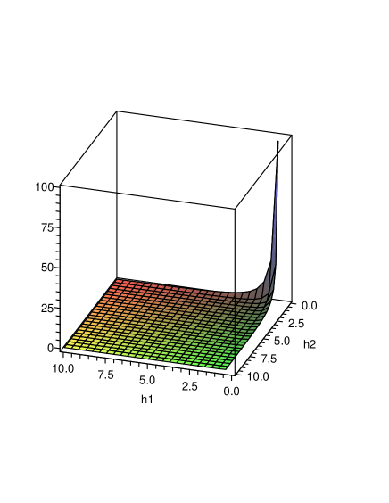
Figure 5: Determinant of the metric tensor as a function of the mass and electric charge scalings $h_{1}$ and $h_{1}$, describing the depletions of an ensemble of evolving statistical systems.

11 Conclusion and Outlook

In this paper, we have explored experimental perspective of the thermodynamic geometry. Our analysis is particularly suitable for the thin film depletion layer formation at a small scale structure formation under the fluctuations of the deposited electric charge and the atomic mass. Keeping in mind the nature of finitely many excited, non-empty $d$/ $f$-orbital heavy materials, we have investigated the detailed mathematical picture of the intrinsic thermodynamic geometric and topological characterizations of the small fluctuation over a depletion layer formation.

Under each adiabatic evolution of the local thermodynamic macro-states, we have examines the nature of (i) electric charge, and mass fluctuations under the respective embeddings, (ii) positivity of the local heat capacities, (iii) global thermodynamic stability of the canonical ensemble under the Gaussian fluctuations of a sequence of the electric charges and depleting masses, and (iv) global charge-mass correlations. Thus, we have offered a detailed experimental perspective of the intrinsic thermodynamic geometry.

For any non-degenerate thermodynamic metric tensor and a regular Gaussian curvature $K(x_{1},x_{2})$, we have generically shown that there are no global phase transitions on $\mathcal{M}_{QM}$. On the other hand, there may exist finitely many critical points, which are predicted to occur at the roots of the determinant of the metric tensor. Such a finite critical set may be given as

$$\mathcal{C}:=\{c_{1},c_{2},\ldots,c_{n}\}$$ (42)

In general dimensions, there may be diverse critical properties of the $\mathcal{M}_{QM}$. For regular $N(x_{1},x_{2})$, we notice in the two dimensions that the global phase transitions only occur precisely over the set $\mathcal{C}$. This classification thus effectively confirms notion of Widom’s spoidal curves [62] and the associated global critical phenomena, which are prone to occur under the metal depletion and it’s thin layer formation.

It is worth mentioning that the order of $R(x_{1},x_{2})$ determines the order of the phase transition in the system. Thus, the general consideration of $\mathcal{M}_{QM}$ makes the function $N(x_{1},x_{2})$ more involved. Specifically, when $N(x_{1},x_{2})$ is a singular function on a patch of the $\mathcal{M}_{QM}$, then the global phase transitions can occur, even if the metric tensor $g_{ij}$ is non-degenerate. In this case, the only requirement to exist a global phase transition is that both the electric charge and the mass fluctuations should be finite and non-zero under a layer formation. From the perspective of numerical analysis, we have proposed a well-defined numerical code of the lattice evolutions. The proposed code corresponds to a non-interacting local statistical system, whenever the chosen equilibrium remains far separated from the underlying ensemble of the equilibria.

To determine the above notions experimentally or within the scope of intrinsic geometric model, we need to specify the sample, which we have described in this paper as the possible local set-up of our model. For an exact surface modeling, one may choose a fined shape of certain slab, such as square/ rectangle, circle, ellipse. It is further possible to chose some quadrilaterals, like cross-quadrilateral, butterfly quadrilateral, bow-tie quadrilateral and other skew quadrilaterals. For a near-surface daily-life modeling, we may add an extra tiny third direction (having a size of few nano-meter to few micro-meter) to the present intrinsic geometric surface modeling. In such cases, one may thus consider a near-surface modeling for the this layer depletion over a fixed desired image, such as table, thin cylinder, thin prism, thin pyramid, thin fridge, thin sheeted stairs, small regulated cone without the tip, thin ellipsoid, and finally any thin shell of radii $r_{1}$ and $r_{2}$ with $r_{1}\sim r_{2}$. It is needless to mention that the present characterization holds for any such possible similar pattern formation. In the sense of the statistical physics [10, 11] and modern aspects of the functional analysis [86], the present exposition offers a microscopic understanding of the thin layer depletion and pattern formation.

The above classes of the shapes are useful in daily-life appliances for the composition of an illusive, high-cost, precious looking objects and the associated materials possibly useful in perspective decorations. Our method is very desirable in determining the quality of thin film coating, and thus in determining the local and the global nature of the coated layer on a low cost material, viz. silica. Following such a characterizing procedure, one may control the quality of thin layer depletion. This can be further useful in producing a durable illusive, stylish, low economic factor, quality-looking products at a desired economic value. Thus, such an investigation leads to several industrial importance, offering a class of possible daily-life appliances, from the application of the intrinsic thermodynamic geometry.

Apart from the above mentioned considerations, the designed method is further applicable to arbitrary shape coating’s on definite low-economic-factor frame, viz. $\mathcal{M}_{QM}$. At the desired scale, such a surface of coatants is a randomly fluctuating surface, which after the equilibration leads to a desired quality quoted shape, at a large scale. Looking after the present experimental set-up’s and associated daily-life demands, we may set-up the scale of the experimental thermodynamic geometry in the order of a few nano-meter to a few micro-meter. Although, the large scale coating are well-explained from the very out-set of the present model, however their present daily-life significance involved are of minor importance, which from the demand based economic perspective, so it might be herewith practically of minor noteworthy to emphasize their details.

To achieve the global quality shape thin layer depletion, one only needs to compute the Gaussian curvature $K(x_{1},x_{2})$. Thereby, one may deduce the topological nature of the stability of underlying structure formation, and global phase-space correlations on $\mathcal{M}_{QM}$. In summary, the thin layer characterizations of desired formation can easily be acquired by studying the local and global properties of fluctuating surfaces, arising under the depletion of the effective electric charge and depletion mass.

References

- [1] F. Weinhold, “Metric geometry of equilibrium thermodynamics”, J. Chem. Phys. 63 , 2479 (1975), DOI:10. 1063/ 1. 431689.
- [2] F. Weinhold, “Metric geometry of equilibrium thermodynamics. II”, Scaling, homogeneity, and generalized Gibbs–Duhem relations, ibid J. Chem. Phys 63 , 2484 ( 1975).
- [3] G. Ruppeiner, “Thermodynamics: A Riemannian geometric model”, Phys. Rev. A 20, 1608 (1979).
- [4] G. Ruppeiner, “Riemannian geometry in thermodynamic fluctuation theory”, Rev. Mod. Phys 67 (1995) 605, Erratum 68 (1996) 313.
- [5] G. Ruppeiner, “Thermodynamic Critical Fluctuation Theory?”, Phys. Rev. Lett. 50, 287 (1983).
- [6] G. Ruppeiner, “New thermodynamic fluctuation theory using path integrals”, Phys. Rev. A 27,1116,1983.
- [7] G. Ruppeiner and C. Davis, “Thermodynamic curvature of the multicomponent ideal gas”, Phys. Rev. A 41, 2200, 1990.
- [8] G. Ruppeiner, “Thermodynamic curvature and phase transitions in Kerr-Newman black holes”, Phys. Rev. D 75, 024037 (2007).
- [9] R. M. Wald, “General Relativity”, University of Chicago Press (Chicago, 1984).
- [10] K. Huang, “Statistical Mechanics”, John Wiley, (1963).
- [11] L. D. Landau, E. M. Lifshitz, “Statistical Physics-I, II”, Pergamon, (1969).
- [12] J. E. Aman, I. Bengtsson, N. Pidokrajt, “Geometry of black hole thermodynamics”, Gen. Rel. Grav. 35 (2003) 1733, arXiv:gr-qc/0304015v1.
- [13] J. E. Aman, N. Pidokrajt, “Geometry of Higher-Dimensional Black Hole Thermodynamics”, Phys. Rev. D 73 (2006) 024017, arXiv:hep-th/0510139v3.
- [14] G. Arcioni, E. Lozano-Tellechea, “Stability and critical phenomena of black holes and black rings”, Phys. Rev. D 72, 104021 (2005).
- [15] M. Santoro, A. S. Benight, “On the geometrical thermodynamics of chemical reactions”, math-ph/0507026.
- [16] J. Shen, R. G. Cai, B. Wang, R. K. Su, “Thermodynamic Geometry and Critical Behavior of Black Holes”, Int. J. Mod. Phys. A 22 (2007) 11-27, arXiv:gr-qc/0512035v1.
- [17] H. B. Callen, “Thermodynamics and an Introduction to Thermostatistics”, Pub. Wiley, New York, (1985).
- [18] L. Tisza, “Generalized Thermodynamics”, Pub. MIT Press, Cambridge, MA (1966),
- [19] L. Andrianopoli, R. D’Auria, S. Ferrara, “Flat Symplectic Bundles of N-Extended Supergravities, Central Charges and Black-Hole Entropy”, arXiv:hep-th/9707203v1.
- [20] S. Ferrara, G. W. Gibbons, R. Kallosh, “Black Holes and Critical Points in Moduli Space”, Nucl. Phys. B 500, 75-93, (1997), arXiv:hep-th/9702103v1 .
- [21] J. P. Gauntlett, J. B. Gutowski, C. M. Hull, S. Pakis, H. S. Reall, “All supersymmetric solutions of minimal supergravity in five dimensions”, Class. Quant. Grav. 20 4587-4634, (2003), arXiv:hep-th/0209114v3.
- [22] S. Bellucci, S. Ferrara, A. Marrani, “Supersymmetric mechanics. Vol. 2, The attractor mechanism and space time singularities”, Lect. Notes Phys. 701,1-225, (2006) .
- [23] S. Bellucci, S. Ferrara, A. Marrani, “Extremal Black Hole and Flux Vacua Attractors”, Lect. Notes Phys. 755, 115, (2008), arXiv:0711.4547.
- [24] S. Bellucci, S. Ferrara, M. Gunaydin, A. Marrani, “SAM Lectures on Extremal Black Holes in d=4 Extended Supergravity. The Attractor Mechanism”, Proceedings of the INFN-Laboratori Nazionali di Frascati School 2007, Springer Proceedings in Physics, Bellucci, S. (Ed.), Vol. 134 (2010), arXiv:0905.3739 [hep-th].
- [25] S. Bellucci, S. Ferrara, A. Marrani, “Attractor Horizon Geometries of Extremal Black Holes”, Proceedings of 17th SIGRAV Conference, Turin, Italy, (2006), arXiv: hep-th/0702019
- [26] D. Gaiotto, A. Strominger and X. Yin, “Superconformal black hole quantum mechanics”, JHEP 0511, 017, (2005), arXiv:hep-th/0412322.
- [27] S. Ferrara, K. Hayakawa, A. Marrani, “Erice Lectures on Black Holes and Attractors”, Fortsch. Phys. 56, 993-1046, (2008), arXiv:0805.2498v2 [hep-th].
- [28] B. L. Cerchiai, S. Ferrara, A. Marrani, B. Zumino, “Duality, Entropy and ADM Mass in Supergravity”, arXiv:0902.3973v2 [hep-th].
- [29] S. Bellucci, S. Ferrara, A. Marrani, A. Yeranyan, “stu Black Holes Unveiled”, Entropy,Vol. 10 (4), p. 507-555, (2008), arXiv:0807.3503v3 [hep-th].
- [30] S. Bellucci, S. Ferrara, A. Marrani, “Attractors in Black”, Fortsch. Phys. 56, 761-785, (2008), arXiv:0805.1310v1 [hep-th].
- [31] G. L. Cardoso, B. de Wit, J. Käppeli, T. Mohaupt, “ Examples of stationary BPS solutions in N=2 supergravity theories with -interactions”, Fortsch. Phys. 49,557, (2001), arXiv:hep-th/ 0012232;
- [32] T. Mohaupt, “Strings, higher curvature corrections, and black holes”, arXiv:hep-th/0512048 .
- [33] T. Mohaupt, “Black Hole Entropy, Special Geometry and Strings”, Fortsch. Phys. 49, 3, (2001), arXiv:hep-th/ 0007195;
- [34] B. de Wit, “Introduction to black hole entropy and supersymmetry”, Proceedings of III Summer School in Modern Mathematical Physics, Zlatibor, (2004),arXiv:hep-th/ 0503211;
- [35] B. de Wit, “Lecture on Black Holes , Topological Strings and Quantum Attractors”, Class. Quant. Grav 23,, S981, (2006), arXiv:hep-th, 0607227;
- [36] A. Sen, “Black Hole Entropy Function, Attractors and Precision Counting of Microstates”, arXiv:hep-th/ 0708.1270;
- [37] P. Kaura, A. Misra, “On the Existence of Non-Supersymmetric Black Hole Attractors for Two-Parameter Calabi-Yau’s and Attractor Equations”, Fortsch. Phys. 54, 1109, (2006), arXiv:hep-th/0607132v3.
- [38] A. Sen, “Black Hole Entropy Function and the Attractor Mechanism in Higher Derivative Gravity,” JHEP 0509, 038, (2005), arXiv:hep-th/ 0506177.
- [39] B. Sahoo, A. Sen, “BTZ Black Hole with Chern-Simons and Higher Derivative Terms”, ” JHEP 0607, 008, (2008), arXiv:hep-th/0601228.
- [40] B. Sahoo, A. Sen, “Higher Derivative Corrections to Non-supersymmetric Extremal Black Holes in N=2 Supergravity,” JHEP 0609, 029, (2006), arXiv:hep-th/0603149.
- [41] A. Sen, “Entropy Function for Heterotic Black Holes,” JHEP 0603, 008, (2006), arXiv:hep-th/ 0508042.
- [42] D. P. Jatkar, A. Sen, “Dyon Spectrum in CHL Models,” JHEP 0604,018, (2006), arXiv:hep-th/ 0510147.
- [43] J. R. David, A. Sen, “CHL Dyons and Statistical Entropy Function from D1-D5 System,” JHEP 0611,072, (2006), arXiv:hep-th/ 0605210.
- [44] R. M. Wald, “Black Hole Entropy is Noether Charge”, Phys.Rev. D 48, 3427, (1993), arXiv:gr-qc/ 9307038.
- [45] V. Iyer, R. M. Wald, “Some Properties of Noether Charge and a Proposal for Dynamical Black Hole Entropy”, Phys.Rev. D50, 846, (1994), arXiv:gr-qc/ 9403028.
- [46] R. M. Wald, Class. Quant.Grav. 16, A177, (1999), arXiv:gr-qc/ 9901033
- [47] A. Dabholkar, N. Iizuka, A. Iqubal, A. Sen, M. Shigemori, “Spinning Strings as Small Black Rings”, JHEP 0704:017, (2007), arXiv:hep-th/0611166v2.
- [48] A. Dabholkar, A. Sen, S. Trivedi, “Black Hole Microstates and Attractor Without Supersymmetry,” JHEP 0701, 09, (2007),arXiv:hep-th/ 0611143.
- [49] A. Sen, “Stretching the Horizon of a Higher Dimensional Small Black Hole,” JHEP 0507, 073, (2005), arXiv:hep-th/0505122 .
- [50] D. Astefanesei, K. Goldstein, R. P. Jena, A. Sen, S. P. Trivedi, “Rotating Attractors”, JHEP 0610, 058, (2006), arXiv:hep-th/ 0606244 .
- [51] A. Sen, “Strong-Weak Coupling Duality in Four Dimensional String Theory”, IJMP A 9, 3707-3750, (1994), arXiv:hep-th/ 9402002.
- [52] D. Astefanesei, K. Goldstein, S. Mahapatra, “Moduli and (un)attractor black hole thermodynamics”, arXiv:hep-th/0611140.
- [53] S. Bellucci, B. N. Tiwari, “On the Microscopic Perspective of Black Branes Thermodynamic Geometry”, Entropy 2010, 12, 2097-2143, arXiv:0808.3921v1 [hep-th].
- [54] T. Sarkar, G. Sengupta, B. N. Tiwari, “Thermodynamic Geometry and Extremal Black Holes in String Theory”, JHEP 0810, 076, 2008, arXiv:0806.3513v1 [hep-th].
- [55] T. Sarkar, G. Sengupta, B. N. Tiwari, “On the Thermodynamic Geometry of BTZ Black Holes”, JHEP 0611 (2006) 015, arXiv:hep-th/0606084v1.
- [56] B. N. Tiwari, “Sur les corrections de la géométrie thermodynamique des trous noirs”, arXiv:0801.4087v1 [hep-th].
- [57] S. Bellucci, B. N. Tiwari, “Thermodynamic Geometry and Hawking Radiation”, [To Appear in JHEP], arXiv:1009.0633v1 [hep-th] .
- [58] L. Bonora, M. Cvitan, Hawking radiation, W-infinity algebra and trace anomalies JHEP 0805, 071, 2008, arXiv:0804.0198v3 [hep-th].
- [59] Baocheng Zhang, Qing-yu Cai, and Ming-sheng Zhan “Hawking radiation as tunneling derived from Black Hole: Thermodynamics through the quantum horizon” http://arXiv.org/abs/0806.2015v1.
- [60] D. Bekenstein, “Information in the holographic universe”, Sci. Am. 289, No. 2, 58-65 (2003).
- [61] G. Ruppeiner, “Riemannian geometric theory of critical phenomena”, Phys. Rev. A 44 3583 (1991).
- [62] B. Widom, “The critical point and scaling theory,” Physica 73, 107 (1973).
- [63] J. T. Yu, “On Relations Between Jacobians and Minimal Polynomials”, Linear Algebra and it’s Applications 221 19 (1995).
- [64] V. Balasubramanian, J. de Boer, V. Jejjala, J. Simon, “The Library of Babel: On the origin of gravitational thermodynamics”, JHEP 0512 (2005) 006, arXiv:hep-th/0508023v2.
- [65] V. Balasubramanian, M. Berkooz, A. Naqvi, M. J. Strassler, “Giant gravitons in conformal field theory”, JHEP 0204, 034 (2002), arXiv:hep-th/0107119.
- [66] V. Balasubramanian, J. de Boer, V. Jejjala, J. Simon, “Entropy of near-extremal black holes in ”, JHEP 0805, 067 (2008), arXiv:0707.3601v2 [hep-th].
- [67] S. Bellucci, B. N. Tiwari, “An Exact Fluctuating 1/2-BPS Configuration”, JHEP 05 (2010) 023, arXiv:0910.5314v1 [hep-th].
- [68] S. Bellucci, B. N. Tiwari, “State-space Manifold and Rotating Black Holes”, arXiv:1010.1427v1 [hep-th].
- [69] S. Bellucci, B. N. Tiwari, “Black Strings, Black Rings and State-space Manifold”, arXiv:10.3832v1 [hep-th].
- [70] R. Emparan, “Rotating circular strings, and infinite non-uniqueness of black rings”, JHEP 0403, 064, (2004), arXiv:hep-th/0402149.
- [71] B. N. Tiwari, “On Generalized Uncertainty Principle”, arXiv:0801.3402v1 [hep-th].
- [72] O. Aharony, S. Minwalla, T. Wiseman, “Plasma-balls in large N gauge theories and localized black holes”, Class. Quant. Grav. 23, 2171, (2006), arXiv:hep-th/0507219v3.
- [73] L. Grant, P. A. Grassi, S. Kim, S. Minwalla, “Comments on 1/16 BPS Quantum States and Classical Configurations”, JHEP 0805, 049, (2008), arXiv:0803.4183v1 [hep-th].
- [74] V. Chandra, R. Kumar, V. Ravishankar, “Hot QCD equations of state and relativistic heavy ion collisions”, Phys. Rev. C 76, 054909, (2007), arXiv:0705.2690v3 [nucl-th].
- [75] V. Chandra, R. Kumar, V. Ravishankar, “Hot QCD equations of state and RHIC”, arXiv:0805.3199v1 [nucl-th].
- [76] V. Chandra, V. Ravishankar, “Viscosity and thermodynamic properties of QGP in relativistic heavy ion collisions”, Eur. Phys. J. C 59, 705, (2009), arXiv:0805.4820v2 [nucl-th]
- [77] S. Bellucci, V. Chandra, B. N. Tiwari, “Thermodynamic Geometry and Free energy of Hot QCD”, To appear in Int. J. Mod. Phys., arXiv:0812.3792v1 [hep-th].
- [78] S. Bellucci, V. Chandra, B. N. Tiwari, “A geometric approach to correlations and quark number susceptibilities”, [Contributed to the Conference on Quark confinement and the hadron spectrum QCHS IX, Madrid, Spain, 30 August 2010 - 03 September 2010. Proceedings will be published by the American Institute of Physics], arXiv:1010.4405v1 [hep-th].
- [79] Thermodynamic Stability of Quarkonium Bound States, S. Bellucci, V. Chandra, B. N. Tiwari, arXiv:1010.4225v1 [hep-th].
- [80] M. Do Carmo, “Differential Geometry of Curves and Surfaces”, Prentice Hall; First edition, ISBN-10: 0132125897, (1976).
- [81] E. D. Bloch, “A First Course in Geometric Topology and Differential Geometry”, Birkhäuser Boston, ISBN 0817638407 (1996).
- [82] A. A. Markov, “Extension of the limit theorems of probability theory to a sum of variables connected in a chain”, reprinted in Appendix B of: R. Howard. Dynamic probabilistic systems, volume 1: Markov Chains, John Wiley and Sons, (1971).
- [83] A. E. Gelfand, A. F. M. Smith, “Sampling-Based Approaches to Calculating Marginal Densities”, J. Am. Stat. Asso. 398 85 (1990).
- [84] M. I. Zelikin, “Hessian of the solution of the Hamilton-Jacobi equation in the theory of extremal problems”, Sb. Math. 195 819 (2004).
- [85] M. Nakahara, “Geometry, Topology and Physics” (Graduate Student Series in Physics), Second edition, Taylor and Francis ISBN 0750306068, (2003).
- [86] W. Rudin, “Functional Analysis”, McGraw-Hill Science/ Engineering/ Mathematics, 2 Edition (1991).