Flexuron, a self-trapped state of electron in crystalline membranes

Abstract

Self-trapping of an electron due to its interaction with bending fluctuations in a flexible crystalline membrane is considered. Due to the dependence of the electron energy on the corrugations of the membrane, the electron can create around itself an anomalously flat (or anomalously corrugated, depending on the sign of the interaction constant) region and be confined there. Using the Feynman path integral approach, the autolocalization energy and the size of the self-trapped state (flexuron) are estimated. It is shown that typically the size of the flexuron is of the order of the wavelength of fluctuations at the border between harmonic and anharmonic regimes. The flexuron states are connected with the fluctuation tail of the electron density-of-states, the asymptotic behavior of this tail being determined by the exponent of the renormalized bending rigidity.

I Introduction

Studies of statistical mechanics in two dimensions nelson have been strongly stimulated recently by the discovery of graphene first , the first truly two-dimensional crystal and the simplest possible membrane. Experimental jannik and theoretical Fas2007 demonstrations of intrinsic ripples on graphene due to thermal bending fluctuations have initiated numerous works on the effect of the ripples on the electronic properties of graphene KG08 ; castroneto ; oppen ; gazit ; VKG ; guinea due to coupling between electronic and lattice degrees of freedom. This coupling originates from several factors, such as the dependence of electron hopping parameters on interatomic distances and on the angles between chemical bonds as well as from the redistribution of electron density in a deformed membrane (see for review Refs. VKG, ; rmp, ).

However, graphene is just the first representative of a huge class of two-dimensional crystals including broad-gap semiconductors such as hexagonal boron nitride pnas , graphane (hydrogenated graphene) graphane and fluorographene fluor1 ; fluor2 . Electrons in such materials are just conventional nonrelativistic quantum particles and not chiral Dirac fermions like in graphene, and one cannot expect there manifestations of exotic effects of corrugations such as gauge fields VKG . At the same time, another interesting physics specific of the two-dimensional case arises which will be the subject of the present work.

It is known since many years that the interaction of a charge carrier in a semiconductor with some order-parameter fluctuations can drastically change its state leading to self-trapping, or autolocalization brinkman ; krivoglaz ; ourTMF1 ; ourJMMM ; ourTMF2 ; nagaev ; dagotto ; AK1 ; AK2 . This phenomenon is of crucial importance, for example, for the phase separation in magnetic semiconductors and colossal magnetoresistance materials ourTMF2 ; nagaev ; dagotto , where the magnetization plays the role of order parameter. Since the band motion of the electron is easier (and, hence, the bandwidth is larger) for a ferromagnetically ordered state the electron in antiferromagnetic or magnetically disordered surroundings creates a ferromagnetic region and turns out to be self-trapped in this region (different names are used for this state, such as spin polaron ourJMMM , ferron nagaev , or fluctuon krivoglaz ). If concentration of electrons is large enough it leads to a formation of ferromagnetic state in the whole crystal, via so called double exchange, otherwise the phase separation happens, all electrons being trapped in the ferromagnetic regions. The crucial mechanism is the dependence of electron hopping parameter on the angle between magnetic moment on neighboring sites brinkman ; ourTMF2 . Importantly, the critical point where fluctuations of the order parameter are the strongest is the most favorable for these “fluctuon” effects ourTMF1 ; ourJMMM ; AK1 ; AK2 .

Since the hopping parameter in a fluctuating membrane depends on the angle between normals castroneto one can expect a similar physics. If the electron motion is the easiest in the flat membrane, self trapping in an anomalously flat region is possible, in the opposite case an anomalously crumpled region can arise. Since membranes are characterized by very strong bending fluctuations and very slow, power-law decay of the corresponding correlation functions nelson the situation is formally similar to that for autolocalization in the critical point in three-dimensional systems. I will study here this autolocalized state which can be called “flexuron”, by analogy with “ferron”, or “fluctuon”. Technically, I will use the path integral approach path1 ; path2 ; path3 as was applied to the fluctuon problem in our previous works ourTMF1 ; ourJMMM ; AK1 ; AK2 . This method is an adaptation of the seminal work by Feynman on the theory of polaron feynman .

It will be shown that the flexuron forms in crystalline membranes at a large enough coupling constant and its size is of the order of the length scale where interactions between bending and stretching modes become important. The number of electron states in the fluctuation tail of the electron density of states where all states are (auto)localized, even without extrinsic disorder, turns out to be proportional to the temperature.

II Description of the model and mean-field analysis

In the continuum medium theory nelson the membrane is described by the out-of-plane-deformation field $h\left(x,y\right)$. The unit normal vector at a given point is

$$\mathbf{n}\left(x,y\right)=\frac{\left(-\frac{\partial h}{\partial x},-\frac{\partial h}{\partial y},1\right)}{\sqrt{1+\left|\nabla h\right|^{2}}}$$ (1)

where $\nabla$ is the two-dimensional gradient. In the ground state, the membrane is supposed to be flat, and all normals are along $z$ direction (Fig. 1a). At finite temperatures, the membrane is fluctuating, and the normals are no more parallel (Fig. 1b). Let us assume, for simplicity, that the electron spectrum is isotropic near the band minimum. Then, by symmetry, the shift of the band edge due to bending fluctuations should be proportional to $\left|\nabla h\right|^{2}$ and the electron Hamiltonian takes the form

$$\mathcal{H}_{e} = -\frac{\hbar^{2}}{2m}\nabla^{2}+g\varphi\left(\mathbf{r}\right),$$

$$\varphi\left(\mathbf{r}\right) = \left|\nabla h\left(\mathbf{r}\right)\right|^{2}$$ (2)

where $\mathbf{r}=(x,y)$, $m$ is the effective mass, and $g$ is the coupling constant, of the order of the electron bandwidth. It can be both positive or negative, as a result of the interplay of different contributions. If the band is narrowed under crumpling, $g>0$; the edge of the spectrum in this case corresponds to a homogeneous state with $\varphi=0$, the energy of this state is $E=0$. We will start from the case of positive $g$; for negative $g$ the Hamiltonian (2) should be modified, to bound the ground-state energy from below. This case will be considered later, in Section 4.

In the mean-field approximation, at finite temperatures the band edge is shifted up by

$$E_{0}=g\langle\left|\nabla h\right|^{2}\rangle$$ (3)

The inclusion of fluctuations, however, changes this conclusion dramatically. For the case of spin polarons, it was demonstrated already by Brinkman and Rice brinkman that the band edges do not depend on the degree of spin disorder. The band is narrowed in antiferromagnetic or magnetically disordered state in comparison with the ferromagnetic one but not due to the shift of the band edges, just the density of states (DOS) becomes larger at the middle of the band and exponentially small near the edges, similar to the so called Lifshitz tails lifshitz in disordered systems. One can expect the same behavior for our case (Fig. 1c). The mean-field energy (3) is, rather, an inflection point of DOS; the states between $E=E_{0}$ and $E=0$ are associated with rare events, namely, correlated fluctuations such that in some large areas the membrane is flat and normals are parallel. The tail of the DOS below $E_{0}$ is associated with flexurons. The autolocalization region becomes larger when the energy goes closer to the band edge $E=0$ (and the edge itself corresponds to the completely flat state of the whole membrane, cf. Refs. brinkman, ; AK1, ).

(a)

(b)

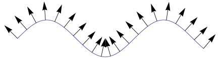
(c)

Figure 1: Ground state of the membrane, all normals (black arrows) are along the $z$ axis (a), and a snapshot of a fluctuating state at finite temperatures (b). Panel (c) shows a sketch of the density of states (DOS) at zero temperature (dashed line), at finite temperatures within mean-field approximation (solid line) and the fluctuation-induced tail (dotted line). We assume $g>0$.

In crystalline membranes, the anharmonic effects are essential, namely, the coupling between bending and stretching modes; without this coupling the membrane turns out to be crumpled at any finite temperatures nelson . In the harmonic approximation which is valid for not too small wavevectors $\mathbf{q}$ of fluctuations, the Fourier component of the normal-normal correlation function $G\left(\mathbf{q}\right)=q^{2}\left\langle\left|h_{\mathbf{q}}\right|^{2}\right\rangle$ at temperature $T$ is given by the expression nelson

$$G\left(\mathbf{q}\right)=\frac{T}{\kappa q^{2}}$$ (4)

where $\kappa$ is the bending rigidity. The use of this expression to calculate $\left\langle\left|\nabla h\right|^{2}\right\rangle$ leads to a logarithmically divergent result. The point is that the expression (4) is not applicable for small enough $q$ where the anharmonic effects become dominant. The coupling between the bending and the stretching phonons in crystalline membranes leads to the renormalization of the bending rigidity and its growth with $q$ decrease. Perturbation analysis shows that the anharmonic effects become dominant at

$$q<q^{*}=\sqrt{3TY/8\pi\kappa^{2}}$$ (5)

where $Y$ is the Young modulus (“Ginzburg criterion” nelson ; Fas2007 ). For smaller $q$,

$$G\left(\mathbf{q}\right)=\frac{A}{q^{2-\eta}q_{0}^{\eta}}$$ (6)

where $q_{0}=\sqrt{Y/\kappa}$ is of the order of inverse interatomic distance and $\eta$ is the exponent of the renormalized bending rigidity. Within the self-consistent screening approximation radz ; gaz1 ; rafa $\eta\simeq 0.821$. Recent Monte Carlo simulations los and functional renormalization group analysis kow ; brag give $\eta\simeq 0.85.$

The factor $A$ can be found from the matching of expressions (4) and (6) at $q=q^{*}$:

$$A=\alpha\left(\frac{T}{\kappa}\right)^{1-\eta/2}$$ (7)

where $\alpha$ is a numerical factor.

With logarithmic accuracy, one finds

$$E_{0}=\frac{Tg\Lambda}{2\pi\kappa}$$ (8)

where $\Lambda=\ln\left(q_{0}/q^{*}\right)\approx\left(1/2\right)\ln\left(\kappa/T\right)$ originates from the cutoff at small $q$ and we assume $T\ll\kappa$ (for example, for graphene $\kappa\simeq 1eV$ Fas2007 ). Thus, within the mean-field approximation, the shift of the band edge is proportional to temperature. Physically this effect is observable (i.e. not hidden by thermal smearing) if $\left|E_{0}\right|>T,$ that is, $\left|g\right|\Lambda\gg\kappa$. Further we will assume that this condition is fulfilled, e.g., due to a large logarithm.

III Fluctuation effects in the case of electron preferring flat surrounding

To take into account the effect of fluctuations on the electron energy spectrum I will use the path integral formalism path1 ; path2 ; path3 , following Refs.ourTMF1, ; ourJMMM, ; AK1, ; AK2, .

The partition function of the whole system (the electron plus the fluctuating field $\varphi$) is represented as

$$Z=\mbox{Tr}e^{-\beta\mathcal{H}_{f}\left(\varphi\right)-\beta\mathcal{H}_{e}\left(\mathbf{r,}\varphi\right)}=Z_{f}\left\langle\mbox{Tr}_{\mathbf{r}}T_{\tau}\exp\left[-\int_{0}^{\beta}\mathcal{H}_{e}\left(\mathbf{r,}\varphi\left(\mathbf{r,}\tau\right)\right)d\tau\right]\right\rangle_{f}$$ (9)

where $\beta=T^{-1}$ is the inverse temperature, $\mathcal{H}_{e}$ is the Hamiltonian (2), $Z_{f}=\mbox{Tr}_{\varphi}e^{-\beta\mathcal{H}_{f}\left(\varphi\right)}$ is the partition function of the field, $\mathcal{H}_{f}$ is the corresponding Hamiltonian, $\varphi\left(\mathbf{r,}\tau\right)=e^{\tau\mathcal{H}_{f}\left(\varphi\right)}\varphi\left(\mathbf{r}\right)e^{-\tau\mathcal{H}_{f}\left(\varphi\right)}$ and

$$\left\langle\mathcal{A}\left(\varphi\right)\right\rangle_{f}=\frac{1}{Z_{f}}\mbox{Tr}_{\varphi}e^{-\beta\mathcal{H}_{f}\left(\varphi\right)}\mathcal{A}\left(\varphi\right)$$ (10)

is the average over the field states. Using the Feynman path-integral approach path1 ; path2 ; path3 ; feynman and taking average over $\varphi$ yields for the electron-only free energy

$$\mathcal{F}=-\frac{1}{\beta}\left(\ln Z-\ln Z_{f}\right)=-\frac{1}{\beta}\ln\int_{\mathbf{r}\left(0\right)=\mathbf{r}\left(\beta\right)}e^{-\mathcal{S}}\mathcal{D}\left[\mathbf{r}\left(\tau\right)\right],$$ (11)

where the effective action of electron is

$$\mathcal{S}\left[\mathbf{r}\left(\tau\right)\right]=\mathcal{S}_{0}\left[\mathbf{r}\left(\tau\right)\right]+\mathcal{S}_{int}\left[\mathbf{r}\left(\tau\right)\right]$$ (12)

and

$$\mathcal{S}_{0}\left[\mathbf{r}\left(\tau\right)\right]=\frac{1}{2}\int\limits_{0}^{\beta}\left(\frac{d\mathbf{r}}{d\tau}\right)^{2}d\tau,$$ (13)

$$\exp\left(-\mathcal{S}_{int}\left[\mathbf{r}\left(\tau\right)\right]\right)=\left\langle\exp\left[-g\int\limits_{0}^{\beta}\varphi\left[\mathbf{r}\left(\tau\right)\right]d\tau\right]\right\rangle_{f}$$ (14)

(we put temporarily $\hbar=m=1$). The average can be formally written as a cumulant expansion

$$\mathcal{S}_{int}=-\sum_{m=1}^{\infty}\frac{g^{m}}{m!}\int_{0}^{\beta}...\int_{0}^{\beta}\mathcal{K}_{m}\left(\mathbf{r}\left(\tau_{1}\right)...\mathbf{r}\left(\tau_{m}\right)\right)d\tau_{1}...d\tau_{m}$$ (15)

where $\mathcal{K}_{m}\left(\mathbf{r}_{1};...;\mathbf{r}_{m}\right)$ are the $m$-th cumulant correlators, defined recursively by

$$\mathcal{K}_{1}\left(\mathbf{r}_{1}\right) =\left\langle\varphi\left(\mathbf{r}_{1}\right)\right\rangle_{f},$$

$$\mathcal{K}_{2}\left(\mathbf{r}_{1};\mathbf{r}_{2}\right) =\left\langle\varphi\left(\mathbf{r}_{1}\right)\varphi\left(\mathbf{r}_{2}\right)\right\rangle_{f}-\mathcal{K}_{1}\left(\mathbf{r}_{1}\right)\mathcal{K}_{1}\left(\mathbf{r}_{2}\right),...$$ (16)

etc.

To estimate the electron free energy $\mathcal{F}$ we use the same trial action as in Refs.ourTMF1, ; ourJMMM, ; AK1, , $\mathcal{S}_{t}=\mathcal{S}_{0}+\mathcal{S}_{pot}$ where

$$\mathcal{S}_{pot}=\frac{\omega^{2}}{4\beta}\int_{0}^{\beta}\int_{0}^{\beta}\left[\mathbf{r}\left(\tau\right)-\mathbf{r}\left(\sigma\right)\right]^{2}d\tau d\sigma,$$ (17)

the oscillator frequency $\omega$ being trial parameter (in contrast with Ref.AK2, ; feynman, we do not introduce any retardation in the trial action since it is important only for the case of quantum fluctuations of the field $\varphi$ which is beyond the scope of the present work). It describes in a translationally invariant way a self-trapped state if $\beta\hbar\omega\gg 1$, in this case the size of the self-trapping region is of the order of the zero-point oscillations of a harmonic oscillator, $l=\sqrt{\hbar/2m\omega}$. The trial action $\mathcal{S}_{t}$ gives an upper estimate of free energy for our problem. The Peierls-Feynman-Bogoliubov inequality reads

$$\mathcal{F}\leq\mathcal{F}_{t}+\frac{1}{\beta}\left\langle\mathcal{S}_{int}-\mathcal{S}_{pot}\right\rangle_{t}$$ (18)

where $\mathcal{F}_{t}$ is the free energy corresponding to the trial action $\mathcal{S}_{t}$, which is equivalent to

$$\mathcal{F} \leq\mathcal{F}_{t}-\frac{\omega^{2}}{4\beta^{2}}\int_{0}^{\beta}\int_{0}^{\beta}\left\langle\left[\mathbf{r}\left(\tau\right)-\mathbf{r}\left(\sigma\right)\right]^{2}\right\rangle_{t}d\tau d\sigma$$

$$-\sum_{m=1}^{\infty}\frac{g^{m}}{m!\beta}\int_{0}^{\beta}...\int_{0}^{\beta}\left\langle\mathcal{K}_{m}\left(\mathbf{r}\left(\tau_{1}\right),...,\mathbf{r}\left(\tau_{m}\right)\right)\right\rangle_{t}\prod_{j=1}^{m}d\tau_{j}$$ (19)

To proceed, we will pass to the Fourier transforms of the cumulants $\mathcal{K}_{m}\left(\mathbf{q}_{1},..,\mathbf{q}_{m-1}\right)$ and take into account that for the Gaussian trial action $\mathcal{S}_{t}$ one has

$$\left\langle\exp\left\{i\sum_{j=1}^{m-1}\mathbf{q}_{j}\left[\mathbf{r}\left(\tau_{j}\right)-\mathbf{r}\left(\tau_{m}\right)\right]\right\}\right\rangle_{t}=$$

$$\exp\left\{-\sum_{j,k=1}^{m-1}\frac{\mathbf{q}_{j}\mathbf{q}_{k}}{4}\left\langle\left[\mathbf{r}\left(\tau_{j}\right)-\mathbf{r}\left(\tau_{m}\right)\right]\left[\mathbf{r}\left(\tau_{k}\right)-\mathbf{r}\left(\tau_{m}\right)\right]\right\rangle_{t}\right\}.$$ (20)

For the autolocalized states the variational parameter $\omega$ satisfies the inequalities $\beta\omega\gg 1$ and $\omega\ll W$ where $W$ is of the order of the electron bandwidth (the last inequality just means that the flexuron size $l=1/\sqrt{2\omega}$ is much larger than the interatomic distance, otherwise our continuum-medium description is not applicable).

Due to the first inequality one has ourJMMM

$$\left\langle\mathbf{r}\left(\tau_{i}\right)\mathbf{r}\left(\tau_{k}\right)\right\rangle_{t}\approx 2l^{2}\delta_{ik}$$ (21)

and Eq.(20) is simplified:

$$\mathcal{F}\leq\frac{\omega}{2}-\sum\limits_{m=1}^{\infty}\frac{1}{m!\beta}\left(g\beta\right)^{m}\sum_{\mathbf{q}_{i}}\mathcal{K}_{m}\left({\mathbf{q}}_{1},...,{\mathbf{q}}_{m-1}\right)\times$$

$$\exp\left[{-\frac{1}{{4}\omega}\sum\limits_{j=1}^{m-1}{\mathbf{q}_{j}^{2}}-\frac{1}{{4}\omega}\left({\sum\limits_{j=1}^{m-1}{\mathbf{q}_{j}}}\right)^{2}}\right].$$ (22)

In harmonic approximation, the second cumulant can be calculated using Wick’s theorem:

$$\mathcal{K}_{2}\left(\mathbf{q}\right)=\sum\limits_{\mathbf{p}}G\left(\mathbf{q}\right)G\left(\mathbf{p-q}\right).$$ (23)

Within the self-consistent screening approximation radz (neglecting vertex corrections) this expression is also supposed to be correct. Note that this approximation is in reasonable agreement with the results of Monte Carlo simulations rafa . We will use it here. Substituting Eqs.(4) and (6) into Eq.(23) one finds

$$\mathcal{K}_{2}\left(\mathbf{q}\right)=\left\{\begin{array}[]{cc}\frac{1}{\pi}\left(\frac{T}{\kappa}\right)^{2}\frac{\ln\left(q/q^{*}\right)}{q^{2}},&q>q^{*}\\ \frac{\alpha^{\prime}}{q_{0}^{2\eta}q^{2-2\eta}}\left(\frac{T}{\kappa}\right)^{2-\eta},&q<q^{*}\end{array}\right.$$ (24)

where $\alpha^{\prime}$ is a numerical factor.

Let us start estimating Eq.(22) in the Gaussian approximation, that is, taking into account only terms with $m=1,2$, then

$$\mathcal{F}\leq E_{0}+\frac{1}{4l^{2}}-\frac{g^{2}}{2T}\sum\limits_{\mathbf{q}}\mathcal{K}_{2}\left(\mathbf{q}\right)\exp\left(-q^{2}l^{2}\right)$$ (25)

Now we have to minimize the right-hand-side of Eq.(25) to find the size of flexuron $l_{0}$ and the autolocalization energy.

Let us assume first that $q^{*}l\ll 1$. In this case one can rewrite Eq.(25) as

$$\mathcal{F}\leq E_{0}+\frac{3TY\hbar^{2}}{32\pi\kappa^{2}m}x-\frac{Tg^{2}}{32\pi^{2}\kappa^{2}}\ln^{2}x,$$ (26)

where $x=\left(q^{*}l\right)^{-2}$ and we have restored the missing constants $\hbar$ and $m$.

The last two terms in the right-hand-side of Eq.(26) are proportional to temperature. The minimum of this function exists if

$$\nu=\frac{g^{2}m}{3\pi Y\hbar^{2}}>\frac{e}{2}$$ (27)

($e\simeq 2.71828...$) which is a criterion of autolocalization in this approximation. Of course it is valid only with an accuracy of some numerical factor since we kept only leading logarithms in our estimations. It is hardly to expect that $\nu$ is much larger than one, thus, an optimal value of $x$ is of the order of unity, beyond the formal limit of the approximation (26). The analysis from the opposite limit, $q^{*}l\gg 1$ gives the same result which is not surprising keeping in mind that the expressions (24) match at $q\approx q^{*}$. Therefore,

$$l_{0} \simeq 1/q^{*}\propto T^{-1/2},$$

$$\mathcal{F}_{opt} \simeq E_{0}-const\cdot T$$ (28)

This is the main result of our consideration, and it is amazingly simple: the size of the self-trapping region is of the order of $1/q^{*}$ (which is much larger than the interatomic distance, so the continuum medium description works). Thus, inhomogeneities induced by electrons in fluctuating membrane should have the same spatial scale as the crossover length from the harmonic to the anharmonic regime.

The higher-order terms in the cumulant expansion in Eq.(22) can be estimated from the expressions in the harmonic regime. Each next couple of the Green functions $G\left(\mathbf{q}\right)$ gives an additional factor $1/q^{2}$, together with additional integration over $\mathbf{q}$ (which can affect the powers of logarithms) and, importantly, the additional small parameter $\left(T/\kappa\right)^{2}$, which is only partially compensated by the additional factor $\beta g$. Thus, the cumulant expansion has a small parameter $Tg/\kappa^{2}$ and the results of the Gaussian approximation are reliable.

A compact analytical expression for the density of states $N(E)$ can be obtained for the Lifshitz tail regime, that is, very close to the true edge of the spectrum $E=0$. To this aim, one can use the method of Ref.AK1, . For the range of energies $E\gg T$, relevant flat regions have a size much larger than $1/q^{*}$, thus, we are in the strongly anharmonic region. From scaling considerations PP , one can postulate that for all $m$, as well as for $m=2$ (cf. Eq.(24)),

$$\mathcal{K}_{m}\left({\mathbf{q}}_{1},...,{\mathbf{q}}_{m-1}\right)=a^{\left(2-2\eta\right)\left(m-1\right)}\mathcal{K}_{m}\left(a{\mathbf{q}}_{1},...,a{\mathbf{q}}_{m-1}\right).$$ (29)

Further consideration just repeats that of Ref.AK1, for the case of XY-model. The result for the Lifshitz tail of the density of states is

$$\ln N\left(E\right)\propto-\left(\frac{T}{E}\right)^{\eta}\left(\ln\frac{T}{E}\right)^{\frac{1}{2\eta+1}},$$ (30)

($E\ll T$). Of course, probing experimentally the states with energies much smaller than the temperature is not an easy task, so the expression (30) is mainly of formal interest.

The number of electron states within the tail between $E=0$ and $E=E_{0}$ can be estimated by a diagrammatic approach suggested in Ref.AK2, , Section 4.3. By analogy with Eq.(152) of that work, one can estimate the electron concentration per atom as

$$n_{c}\approx gT/\kappa^{2}.$$ (31)

IV Fluctuation effects in the case of electrons preferring crumpled surrounding

Consider now the case of a negative coupling constant which physically means that corrugations result in a gain of electron energy. The Hamiltonian (2) cannot be used here since its spectrum is not bounded from below. Instead we will use the Hamiltonian

$$H=-\frac{\hbar^{2}}{2m}\nabla^{2}+\frac{g}{2}\left(\varphi\left(\mathbf{r}\right)-\varphi_{0}\right)^{2}$$ (32)

where $g$ is still positive and $\varphi_{0}$ is the value of $\left|\nabla h\right|^{2}$ optimal for electron hopping; the coupling constant is now $g_{0}=-g\varphi_{0}$, and $E=0$ is still the lowest possible energy. Using the Hubbard-Stratonovich transformation, the partition function of electron in a given field $\varphi\left(\mathbf{r}\right)$ can be represented as (again, $\hbar=m=1$):

$$Z_{e} = \int\mathcal{D}\mathbf{r}\left(\tau\right)\exp\left[-\frac{1}{2}\int\limits_{0}^{\beta}\left(\frac{d\mathbf{r}\left(\tau\right)}{d\tau}\right)^{2}d\tau-\frac{g}{2}\int\limits_{0}^{\beta}\left[\varphi\left(\mathbf{r}\left(\tau\right)\right)-\varphi_{0}\right]^{2}d\tau\right]=$$ (33)

$$\int\mathcal{D\gamma}\left(\tau\right)\int\mathcal{D}\mathbf{r}\left(\tau\right)\exp\left[-\frac{1}{2}\int\limits_{0}^{\beta}\left(\frac{d\mathbf{r}\left(\tau\right)}{d\tau}\right)^{2}d\tau-i\int\limits_{0}^{\beta}\mathcal{\gamma}\left(\tau\right)\left[\varphi\left(\mathbf{r}\left(\tau\right)\right)-\varphi_{0}\right]d\tau-\frac{1}{2g}\int\limits_{0}^{\beta}\mathcal{\gamma}^{2}\left(\tau\right)d\tau\right]$$

Repeating the derivation of Eq.(19) we will find the only difference: $g^{m}$ is replaced by the product $i^{m}\prod_{j=1}^{m}\gamma\left(\tau_{j}\right)$ averaged over fluctuations of the Gaussian field $\gamma(\tau)$.

Continuing the transformations leading from Eq.(19) to Eq.(22) one obtains formally the same equation but with the replacement of $g$ by $i\gamma_{0}$,

$$\gamma_{0}=\frac{1}{\beta}\int\limits_{0}^{\beta}\gamma(\tau)d\tau.$$ (34)

At the end, as follows from Eq.(33), one has to average the result over the Gaussian random static field $\gamma_{0}$ distributed with the probability function

$$P\left(\gamma_{0}\right)=\sqrt{\frac{\pi\beta}{2g}}\exp\left(-\frac{\beta\gamma_{0}^{2}}{2g}+i\beta\gamma_{0}\varphi_{0}\right)$$ (35)

An optimal value of this random field corresponding to the extremum of the exponent in Eq.(35) is equal to $ig\varphi_{0}$ and the fluctuations are of the order of $\sqrt{gT}$, that is, negligible if $T\ll g\varphi_{0}$. Thus, the effective coupling constant for the fluctuation contributions is just equal to $g_{0}$. All the conclusions of the previous section about the size of flexuron and criterion of autolocalization remain valid. The mean-field expression for the shift of the band edge is now different. As follows directly from Eq.(32)

$$E_{0}=\frac{g}{2}\left(\varphi_{0}^{2}-\langle\varphi^{2}\rangle\right)^{2}.$$ (36)

V Discussion and conclusions

We have shown that the electron can be self-trapped by bending fluctuations assuming that the parameter $\nu$, Eq.(27) is large enough. One can expect $g$ to be of the order of the electron bandwidth $W$ (cf. the discussions for graphene reviewed in Ref.VKG, ). For the Young modulus a natural estimation is $Y\approx E_{coh}/a^{2}$ where $E_{coh}$ is a cohesive energy and $a$ is a lattice constant. For covalently bonded membranes (such as graphene or h-BN) $W\approx E_{coh}$. This means that the effective mass should be of the order of the free electron mass, and therefore it is hardly to expect the formation of flexuron for, e.g., gapped graphene with a mass $m\ll\hbar^{2}/Wa^{2}$. On the other hand, the criterion of autolocalization should be easy to fulfill for a soft membrane with $E_{coh}\ll W$.

Assuming that we are in the regime of the autolocalization, the electron injection into crystalline membranes at finite temperatures does not result in the conductivity, the states will be (auto)localized, even without external disorder. This will be the case till the whole fluctuation tail will be occupied. The number of the states in the fluctuation tail is given by Eq.(31), so the transition to the conducting states happens at $n=n_{c}\propto T$. The higher the temperature the more electrons should be injected.

Strictly speaking, the flexuron states are completely localized only if one assumes that the fluctuations are static. In an ideal system, the flexuron can move together with the anomalously corrugated region, but very slowly, for typical phonon times (cf. the discussion for the case of fluctuon krivoglaz ). One can expect, however, that even very weak extrinsic disorder will localize so slow particle.

If the flexuron forms, its size is of the order of $1/q^{*}$ where $q^{*}$ (5) is a crossover point from harmonic to anharmonic regime, so, the bending fluctuations are stabilized by electrons just at the border of the strong anharmonicity.

A very interesting issue for future studies is the case of finite electron (flexuron) concentrations. By analogy with magnetic semiconductors, one can expect a tendency to the phase separation and electron droplet formation ourTMF2 ; nagaev ; dagotto . Electronic mechanisms of stabilization of corrugations were discussed in a context of graphene castroneto ; gazit ; guinea but in a broad-gap semiconductors considered here physics should be essentially different. Probably, the flexuron formation is a proper term in this case.

References

- (1) Statistical Mechanics of Membranes and Surfaces, edited by D. R. Nelson, T. Piran, and S. Weinberg (World Scientific, Singapore, 2004).
- (2) K. S. Novoselov, A. K. Geim, S. V. Morozov, D. Jiang, Y. Zhang, S. V. Dubonos, I. V. Grigorieva, and A. A. Firsov, Science 306, 666 (2004).
- (3) J. C. Meyer, A. K. Geim, M. I. Katsnelson, K. S. Novoselov, T. J. Booth, and S. Roth, Nature 446, 60 (2007).
- (4) A. Fasolino, J. H. Los, and M. I. Katsnelson, Nat. Mater. 6, 858 (2007).
- (5) M. I. Katsnelson and A. K. Geim, Philos. Trans. R. Soc. London, Ser. A 366, 195 (2008).
- (6) E.-A. Kim and A. H. Castro Neto, Europhys. Lett. 84, 57007 (2008).
- (7) E. Mariani and F. von Oppen, Phys. Rev. Lett. 100, 076801 (2008).
- (8) D. Gazit, Phys. Rev. B 80, 161406 (2009).
- (9) M. A. H. Vozmediano, M. I. Katsnelson, and F. Guinea, Phys. Rep. 496, 109 (2010).
- (10) P. San-Jose, J. Gonzalez, and F. Guinea, arXiv:1009.1285.
- (11) A. H. Castro Neto, F. Guinea, N. M. R. Peres, K. S. Novoselov, and A. K. Geim, Rev. Mod. Phys. 81, 109 (2009).
- (12) K. S. Novoselov, D. Jiang, F. Schedin, T. J. Booth, V. V. Khotkevich, S. V. Morozov, and A. K. Geim, Proc. Natl. Acad. Sci. U.S.A. 102, 10451 (2005).
- (13) D. C. Elias, R. R. Nair, T. M. G. Mohiuddin, S. V. Morozov, P. Blake, M. P. Halsall, A. C. Ferrari, D. W. Boukhvalov, M. I. Katsnelson, A. K. Geim, and K. S. Novoselov, Science 323, 610 (2009).
- (14) J. T. Robinson, J. S. Burgess, C. E. Junkermeier, S. C. Badescu, T. L. Reinecke, F. K. Perkins, M. K. Zalalutdniov, J. W. Baldwin, J. C. Culbertson, P. E. Sheehan, and E. S. Snow, Nano Lett. 10, 3001 (2010).
- (15) R. R. Nair, W. C. Ren, R. Jalil, I. Riaz, V. G. Kravets, L. Britnell, P. Blake, F. Schedin, A. S. Mayorov, S. Yuan, M. I. Katsnelson, H. M. Cheng, W. Strupinski, L. G. Bulusheva, A. V. Okotrub, I. V. Grigorieva, A. N. Grigorenko, K. S. Novoselov, and A. K. Geim, arXiv:1006.3016; to appear in Small.
- (16) W. F. Brinkman and T. M. Rice, Phys. Rev. B 2, 1324 (1970).
- (17) M. A. Krivoglaz, Uspekhi Fiz. Nauk 111, 617 (1973) [Engl. Transl.: Sov. Phys. Uspekhi 16, 856 (1973)].
- (18) M. I. Auslender and M. I. Katsnelson, Teor. Matem. Fizika 43, 261 (1980) [Engl. Transl.: Theor. Math. Phys. 43, 450 (1980)].
- (19) M. I. Auslender and M. I. Katsnelson, J. Magn. Magn. Mater. 241, 117 (1981).
- (20) M. I. Auslender and M. I. Katsnelson, Teor. Matem. Fizika 51, 436 (1982); M. I. Auslender and M. I. Katsnelson, Solid State Commun. 44, 387 (1982).
- (21) E. L. Nagaev, Physics of Magnetic Semiconductors (Mir, Moscow, 1983); E. L. Nagaev, Phys. Rep. 346, 388 (2001).
- (22) E. Dagotto, T. Hotta, and A. Moreo, Phys. Rep. 344, 1 (2001).
- (23) M. I. Auslender and M. I. Katsnelson, Phys. Rev. B 72, 113107 (2005).
- (24) M. I. Auslender and M. I. Katsnelson, Ann. Phys. (N.Y.) 321, 1762 (2006).
- (25) R. P. Feynman and A. R. Hibbs, Quantum Mechanics and Path Integrals (McGraw Hill, New York, 1965).
- (26) L. S. Schulman, Techniques and Applications of Path Integration (Wiley, New York, 1981).
- (27) H. Kleinert, Path Integrals in Quantum Mechanics, Statistics and Polymer Physics (World Scientific, Singapore, 1995).
- (28) R. P. Feynman, Phys. Rev. 97, 660 (1955).
- (29) I. M. Lifshitz, S. A. Gredeskul, and L. A. Pastur, Introduction to the Theory of Disordered Systems (Wiley, New York, 1988).
- (30) P. Le Doussal and L. Radzihovsky, Phys. Rev. Lett. 69, 1209 (1992).
- (31) D. Gazit, Phys. Rev. E 80, 041117 (2009).
- (32) K. V. Zakharchenko, R. Roldán, A. Fasolino, and M. I. Katsnelson, Phys. Rev. B 82, 125435 (2010).
- (33) J. H. Los, M. I. Katsnelson, O. V. Yazyev, K. V. Zakharchenko, and A. Fasolino, Phys. Rev. B 80, 046808 (2009).
- (34) J.-P. Kownacki and D. Mouhanna, Phys. Rev. E 79, 040101 (2009).
- (35) F. L. Braghin and N. Hasselmann, Phys. Rev. B 82, 035407 (2010).
- (36) A. Z. Patashinskii and V. L. Pokrovskii, Fluctuation Theory of Phase Transitions (Pergamon, New York, 1979).