Fermion- and spin-counting in strongly correlated systems in and out of thermal equilibrium

Abstract

Atom counting theory can be used to study the role of thermal noise in quantum phase transitions and to monitor the dynamics of a quantum system. We illustrate this for a strongly correlated fermionic system, which is equivalent to an anisotropic quantum XY chain in a transverse field, and can be realized with cold fermionic atoms in an optical lattice. We analyze the counting statistics across the phase diagram in the presence of thermal fluctuations, and during its thermalization when the system is coupled to a heat bath. At zero temperature, the quantum phase transition is reflected in the cumulants of the counting distribution. We find that the signatures of the crossover remain visible at low temperature and are obscured with increasing thermal fluctuations. We find that the same quantities may be used to scan the dynamics during the thermalization of the system.

I Introduction

In the past decade it became clear that the most important challenges of physics of ultracold atoms overlap essentially with those of condensed matter physics, and concern strongly correlated quantum states of many body systems. In fact, ultracold fermionic and bosonic atoms in optical lattices mimic strongly correlated systems, that can be perfectly described by various Hubbard or spin models with rich phase diagrams adp .

Amazingly, atomic physics may address questions concerning both static and dynamical properties of such systems. In the context of statics, the goal is to quantum engineer, i.e. to prepare, or reach interesting quantum phases or states, and then to detect their properties. Many examples of such exotic phases pertaining to quantum magnetism based on super-exchange interactions are now within experimental reach expe ; expe2D . Also, the signatures of itinerant ferromagnetism in the absence of the lattice structure have been recently reported for a system of spin 1/2 fermions expek .

Despite the progress of experimental techniques, the preparation and detection of quantum magnetism is always obscured by the unavoidable noise and thermal effects. These are particularly important in low dimensional systems, and, in particular, in one dimension (1D) where no long range order can exist at $T>0$. It is therefore highly desirable to design detection methods that will allow to observe the signatures of strong correlations and quantum phase transitions (QFT) at $T>0$. The first goal of this paper is to demonstrate that atom counting may be used to detect signatures of QFTs at $T>0$. To this aim we analyze a paradigmatic example of a strongly correlated system: a system of fermions in a 1D optical lattice.

Remarkable long time scales in ultracold atom experiments allow to monitor the dynamics of the system directly. In the context of dynamics, one goal is to observe the time evolution of the system under some perturbation as the system approaches a stationary state. In this context various fundamental questions can be addressed. For instance, does the system, which can be very well regarded as closed, thermalize after initial perturbation (sudden quench) Sengupta ; sensother ; Muramatsu ; Eisert ; ortiz ; Ciracbanuls ? What is the difference between thermal and non thermal dynamics? What kinds of interesting dynamical processes involving a coupling to a specially designed heat bath can be realized? Can one realize state engineering using open system dynamics env ? The second goal of this paper is thus to study atom counting during dynamic evolution. In particular, we compute the atom counting distributions as a function of time when the analyzed 1D system of fermions approaches the quantum Boltzmann-Gibbs thermal equilibrium state at certain $T>0$. We show how the thermalization process can be monitored by observing the cumulants of the counting distribution. In principle, the methods allows thus to distinguish thermal dynamics from non-thermal one.

Counting of particles is one of the most important techniques of characterization of quantum mechanical states of many body systems. Photon counting, whose theory was developed in the seminal works Glauber-seminal , allows for the full characterization of quantum light sources. More recently, the counting statistics of electrons has been used to characterize mesoscopic devices electrons ; bednorz ; belzig ; bbb ; oppen ; electrons2 ; schonhammer . In both mentioned cases, the particles considered are non-, or practically noninteracting. In this paper, in contrast, we consider strongly correlated atomic systems Sachdev . Counting statistics of atoms has been suggested as a technique to detect and distinguish various quantum phases of spin and fermionic systems demler ; counting ; maciejlewenstein ; fermiones ; bruder2 . Atom counting can be realized in several manners (for early experiments, see shimizu ). One method concerns metastable atoms, such as metastable Helium Helium - the atoms are released here from the trap, so counting is preceded by essentially ballistic expansion of the atomic wave functions. With the recent development of high-resolution optical imaging systems, single atoms can be detected with near-unit fidelity on individual sites of an optical lattice expeg ; expeb . This makes available the counting distributions of atoms in situ in the lattice. On the other hand, spin counting techniques Sorensen allow for the measurement of the average and fluctuations of the spin number also in situ in cold atomic samples. These techniques can be extended to account for spatial resolution tobenat and give access to the Fourier components of the spin distribution Troscilde . With the help of superlattice configurations, one may address the atoms locally, probing e.g. every second site tobenat . In this work we focus on in situ methods, leaving the discussion of the interplay of atomic cloud expansion and atom counting to a separate publication.

Despite the fact that in experimental conditions noise (thermal or non-thermal) is always present, so far atom counting has been mainly considered at zero temperature and in the absence of non-thermal noise demler ; counting ; fermiones ; bruder2 ; maciejlewenstein , In particular, in Ref. counting , we have used atom counting theory to study a system of fermions in a one-dimensional (1D) optical lattice. We have shown that the critical behavior of the system, and in particular formation of fermionic pairs, is reflected in the cumulants of the counting distribution. Here, we consider the counting distribution of the same fermionic system, but we now take into account the effect of thermal noise, both by considering the effects of temperature when the system is in an equilibrium state and by that of thermalization when the system is attached to a model heat bath. Fermionic pair breaking induced by thermal noise is clearly reflected in the counting distribution function. We find also that the signatures of the crossover between different phases remain visible at low temperature, and we show how they fade out as the temperature increases.

The paper is organized as follows. In Sec. II, we provide a description of the fermion and spin system that we consider. In section III we review the counting theory for a fermionic system, and show how the counting distribution can be obtained from a simple recursive formula. Details of how to derive the counting distribution in terms of a generating function are shown in the Appendix. In section IV, we study the counting statistics of the system at thermal equilibrium at non-zero temperatures. First, in subsection IV.1, we present the counting distribution at zero temperature for reference. Then, in subsection IV.2, we analyze how thermal noise affects the atom number distributions, especially in the vicinity of the quantum phase transition, or better to say cross-over. In Sec. V, we calculate the atom number distributions during a model thermalization process, in which the system is coupled to a heat bath via the exchange of collective quasi-particles. Such couplings, and the resulting open system dynamics are not strictly speaking local. In Sec. V.2 we analyze, however, the nature of these couplings more closely, and show that they can be well approximated by a physically feasible model of local exchange of atoms between the system and the reservoir. We summarize our results in Sec. VI.

II Fermi Gas in a 1D optical lattice

Quantum degenerate fermionic atoms trapped in optical lattices mifermi may become superfluid if there are attractive interactions between atoms trapped in two different hyperfine states fermisflat . Attractive fermions form pairs analogous to Cooper pairs in superconductors. A one component system of fermions trapped in the same hyperfine state may also become superfluid though not in s-wave configurations. Such a system, in the 1D case, can be described by the Hamiltonian ($\hbar=1$)

$$\hat{H} = -J\sum_{j=1}^{N}(\hat{c}_{j}^{\dagger}\hat{c}_{j+1}+\gamma\hat{c}_{j}^{\dagger}\hat{c}_{j+1}^{\dagger}+h.c.-2g\hat{c}_{j}^{\dagger}\hat{c}_{j}+g).$$

Here, $\hat{c}_{j}^{\dagger}$ denotes the creation of a fermion on site $j$, $N$ is the number of sites, $J$ is the energy associated to fermion tunneling to nearest-neighbor lattice sites, $g$ is proportional to the chemical potential of the system and $\gamma$ accounts for the formation of pairs within consecutive sites. A Fourier transform shows that this corresponds to the formation and destruction of pairs of opposite momentum (see xymodel ; Sachdev ). A Bogoliubov transformation diagonalizes the Hamiltonian in Eq. (LABEL:eq-ham1), which can be written up to a zero energy shift in terms of the quasiparticle excitations $\hat{d}_{k}$,

$$\hat{H}=\sum_{k=1}^{N/2}\hat{H}_{k}=\sum_{k=1}^{N/2}E_{k}\hat{n}^{d}_{k},$$ (2)

where

$$\hat{n}^{d}_{k}=\hat{d}_{k}^{\dagger}\hat{d}_{k}+\hat{d}_{-k}^{\dagger}\hat{d}_{-k}$$ (3)

$$\hat{d}_{k}=u_{k}\hat{c}_{k}-iv_{k}\hat{c}_{-k}^{\dagger},\,\,\,\,\,\,d_{k}^{\dagger}=u_{k}\hat{c}_{k}^{\dagger}+iv_{k}\hat{c}_{-k},$$ (4)

$$\hat{c}_{k}^{\dagger}=\frac{1}{\sqrt{N}}\sum_{j=1}^{N}\exp(ij\Phi_{k})\hat{c}_{j}^{\dagger},$$ (5)

$$u_{k}=\cos{\frac{\theta_{k}}{2}},\,\,\,\,\,\,v_{k}=\sin{\frac{\theta_{k}}{2}},$$ (6)

$$E_{k}=J\sqrt{(\cos{\Phi_{k}}-g)^{2}+\gamma^{2}\sin^{2}{\Phi_{k}}},$$ (7)

$$\tan{\theta_{k}}=\frac{\gamma\sin{\Phi_{k}}}{\cos{\Phi_{k}}-g},$$ (8)

and $\Phi_{k}=2\pi k/N$. In order to recover the Hamiltonian (LABEL:eq-ham1), for $(\cos\Phi_{k}-g)<0$ the solution of Eq. (8) is taken from the ($\frac{\pi}{2},\frac{3\pi}{2}$)-branch of the tangent, whereas for $(\cos\Phi_{k}-g)<0$ it is taken from the ($-\frac{\pi}{2},\frac{\pi}{2}$)-branch.

In the non-interacting case, one can clearly see that there are two different regimes. For $\gamma=0$ the momentum space representation of Eq. (LABEL:eq-ham1), $\hat{H}_{k}=2[\cos(\Phi_{k})-g]\hat{c}_{k}^{\dagger}\hat{c}_{k}$, is recovered up to a constant term. For small transverse field $g\ll 1$, the energy gap of the particles involved is positive. For high transverse field $g\gg 1$, it is negative and it vanishes at the critical point $g=1$. It can be seen from Eq. (6) that the coefficients $u_{k}^{2}$ and $v_{k}^{2}$ change their roles at the phase transition such that on one side of the critical point, the number operator of the quasiparticles $\hat{d}_{k}^{\dagger}\hat{d}_{k}$ corresponds to $\hat{c}_{k}^{\dagger}\hat{c}_{k}$, whereas on the other side it corresponds to $\hat{c}_{k}\hat{c}_{k}^{\dagger}$. Finite interactions $\gamma$ between the fermions lead to the formation of fermionic pairs within consecutive sites but the main character of the phase transition at $g=1$ remains essentially unchanged .

Quantum phase transitions are only well defined at zero temperature. Thermal fluctuations lead to an exponential decay of the order parameter and only a crossover between phases remain. For the system under consideration the critical point $g=1$ at $T=0$ extends for finite $T$ to a quantum critical crossover region where the energy gap is smaller than the thermal fluctuations, i.e. $|J(1-g)|<k_{B}T$ Sachdev .

The system considered here (Eq. (LABEL:eq-ham1)) is also interesting because it is equivalent to the anisotropic quantum XY spin model xymodel . Using the Jordan-Wigner transformation jw ; Sachdev , one can transform it into

$$H_{xy}=-J\sum_{j=1}^{N}\left[(1+\gamma)S_{j}^{x}S_{j+1}^{x}+(1-\gamma)S_{j}^{y}S_{j+1}^{y}+gS_{j}^{z}\right],$$ (9)

where $S_{j}^{\alpha}$ are the spin $1/2$ operators at site $j$, $J$ is the coupling strength, $0<\gamma<1$ is the anisotropy parameter, and $g$ is the parameter of the transverse field. The case $\gamma=1$ corresponds to the Ising model in a transverse field. For $\gamma=0$, the system corresponds to the isotropic XY-model or XX-model. For this value, the Jordan-Wigner transformation is ill-defined and one cannot map it to the fermionic Hamiltonian Eq.(LABEL:eq-ham1). We study the phase transition with respect to the parameter $g$, where the extreme cases $g=0$ and $g=\infty$, correspond to systems with no external field and with no interactions, respectively. The phase transition between the states with different orientations of the magnetization takes place at $g=1$. For small transverse fields $g<1$, the ground state has magnetic long-range order and the excitations correspond to kinks in domain walls. For high transverse fields $g>1$, the system is in a quantum paramagnetic state.

III Fermion Counting Statistics

Before presenting our calculations of the counting distribution for a system of fermions at finite temperature, we would like to remind ourselves of some basics of photon and atom counting statistics. The theoretical analysis of the counting process of photons registered on a photodetector was first developed in Glauber . In such a process, a photon is annihilated and a photoelectron is emitted. This photoemission triggers a further ionization process, leading to a macroscopic current that is then measured. This theoretical framework can be extended for counting atoms directly using multichannel plates or in-situ counting techniques, both for bosons and fermions Cahill_Glauber . In the detection process, the particles are absorbed by the detector. The counting distribution can thus be derived from the master equation that describes the interaction between the system and the detector with efficiency $\varepsilon$ (see the Appendix). The probability $p(m)$ of counting $m$ particles is given by

$$p(m)=\frac{(-1)^{m}}{m!}\frac{d^{m}}{d\lambda^{m}}\mathcal{Q}\Big{|}_{\lambda=1},$$ (10)

where we have used the generating function

$$\mathcal{Q}(\lambda)=\mbox{Tr}(\rho:e^{-\lambda\mathcal{I}}:).$$ (11)

Assuming that the counting process is much faster than the dynamics of the system, the time independent intensity registered at the detector is $\mathcal{I}=\kappa\sum_{j=1}^{N}\hat{c}_{j}^{\dagger}\hat{c}_{j}$, where $\kappa=1-\exp({-\varepsilon\tau})$ and $\tau$ denotes the detection exposure time. Using the anticommutation relations for fermions we obtain

$$\mathcal{Q}(\lambda) = \mbox{Tr}(\rho\prod_{k=1}^{N/2}(1-\lambda\kappa\hat{c}_{k}^{\dagger}\hat{c}_{k})(1-\lambda\kappa\hat{c}_{-k}^{\dagger}\hat{c}_{-k})).$$ (12)

The dynamics mixes only $k$ and $-k$ fermionic excitations $\hat{d}_{k}$ so that we can separate the density matrix $\rho=\prod_{k}\rho_{k}$ and neglect the terms which do not conserve the number of excitations to obtain

$$\mathcal{Q}(\lambda)=\prod_{k=1}^{N/2}\big{(}1-\lambda\kappa A_{k}+\lambda^{2}\kappa^{2}B_{k}\big{)},$$ (13)

where

$$A_{k} = \hbox{Tr}(\rho_{k}\left[u_{k}^{2}\hat{n}^{d}_{k}+v_{k}^{2}(\hat{d}_{k}\hat{d}_{k}^{\dagger}+\hat{d}_{-k}\hat{d}_{-k}^{\dagger})\right])$$

$$B_{k} = \hbox{Tr}(\rho_{k}\left[u_{k}^{2}\hat{d}_{k}^{\dagger}\hat{d}_{k}\hat{d}_{-k}^{\dagger}\hat{d}_{-k}+v_{k}^{2}\hat{d}_{-k}\hat{d}_{-k}^{\dagger}\hat{d}_{k}\hat{d}_{k}^{\dagger}\right]).$$ (14)

We use Eq. (10) to calculate the counting distribution from the generating function in Eq. (13) and obtain

$$p(m)=\frac{(-1)^{m}}{m!}\frac{d^{m}}{d\lambda^{m}}\Big{[}\prod_{k=1}^{N/2}\big{(}1-\lambda\kappa A_{k}+\lambda^{2}\kappa^{2}B_{k}\big{)}\Big{]}_{\lambda=1}.$$ (15)

Using the generalized Leibniz rule, we derive counting a recurrence relation to calculate the counting distribution for a system with $M+1$ pairs of modes from the distribution of a system with $M$ pairs of modes

$$p(m,M+1) = \sum_{i=0}^{2}{\cal P}_{i}p(m-i,M).$$ (16)

Here ${\cal P}_{i}$ denotes the probability of detecting $i$ particles in the two modes $M+1$ and $-(M+1)$ that is given by

$${\cal P}_{0} = 1-\kappa A_{M+1}+\kappa^{2}B_{M+1},$$

$${\cal P}_{1} = \kappa A_{M+1}-2\kappa^{2}B_{M+1},$$

$${\cal P}_{2} = 1-{\cal P}_{0}-{\cal P}_{1}.$$ (17)

Using the recursive relation Eq. (16), the counting distribution for an arbitrarily large system can be calculated from the counting distributions of a two mode system. We thus only need to calculate the expressions $A_{k}$ and $B_{k}$ in Eq. (14) and use Eqs. (16-17) to obtain the counting distributions of the fermionic system Eq.(LABEL:eq-ham1) with an arbitrary number of sites.

As mentioned above, the fermionic operators are related to spin operators by the Jordan-Wigner transform. The fermion counting distribution is therefore, up to a constant, equivalent to the counting distribution of the spins in $z$-direction in the transverse XY-model in Eq. (9). We can thus use the above to calculate the counting distributions of the anisotropic XY model in a transverse field for a system of any size $N$. Experimentally, the spin number distribution and its fluctuations can be inferred from the expectation value and fluctuations of the polarization of the light that has interacted with a cold atomic sample Sorensen . This spin polarization spectroscopic technique can be also extended to account for spatial resolution of the spin distributions tobenat .

IV Counting statistics in the presence of thermal noise

In real counting experiments, there are typically a variety of noise sources that may affect the system. In this section we study the influence of thermal noise on the counting distributions of the 1D fermi system in Eq. (LABEL:eq-ham1). We analyze the counting distributions along the crossover between the different regions of the phase diagram. We first review the results for the zero temperature case and then turn our discussion to the case with thermal fluctuations.

IV.1 Counting statistics at zero temperature

At zero temperature, the ground state of the system Hamiltonian Eq. (2) is the vacuum state of $\hat{d}_{k}$ excitations. The expressions $A_{k}$ and $B_{k}$ in Eq. (14) are thus given by

$$A_{k}=2\kappa v_{k}^{2}$$

$$B_{k}=\kappa^{2}v_{k}^{2}.$$ (18)

Inserting these into the equations for the two-mode probabilities ${\cal P}_{i}$ in Eq. (17), we obtain the probabilities of finding $0$, $1$ or $2$ particles in a system with one pair of modes

$$p(0,1)=1-2\kappa(v_{1}^{2}+\kappa^{2}v_{1}^{2})$$

$$p(1,1)=2\kappa v_{1}^{2}-2\kappa^{2}v_{1}^{2}$$

$$p(2,1)=\kappa^{2}v_{1}^{2}.$$ (19)

The counting distribution can now be calculated for an arbitrary number of modes using the recurrence relation Eq. (16). In fig. 1 a , we plot the counting probability distribution for the Ising model ($\gamma=1$) at zero temperature with no transverse field ($g=0$) and perfect detection efficiency. We consider a system with zero excitations and $N=1000$ sites. The probability distribution is centered around a mean value $\bar{m}=500=N/2$ particles and its standard deviation $\sigma=50$ such that $\sigma^{2}=N/4$. As was observed in counting , the pairing that is present in the system hamiltonian Eq. (LABEL:eq-ham1) only allows for the detection of pairs of particles and thus leads to a zero probability of finding an odd number of particles. In counting , this splitting of the counting distribution between even and odd values was shown to disappear for decreasing detector efficiency $\kappa$. In the next section Sec. IV.2, we use this feature of the counting distribution to study the influence of thermal fluctuations on the stability of the fermion pairs. In fig. 1 b, we plot the mean $\bar{m}$ and variance $\sigma^{2}$ of the counting distribution for different values of the transverse field $g$. The mean number of particles increases with increasing transverse field $g$. The variance is constant with $g$ up to the critical point, when it decreases with increasing $g$. The phase transition at $g=1$ is clearly visible both in the mean and in the variance. In counting , we studied the behavior of the counting distribution for different values of the anisotropy parameter $\gamma$ and the detection efficiency $\kappa$. We found that the characteristic behavior of the mean and variance as shown in fig 1 b) is similar when $\gamma$ varies from $0$ to $1$. We further found that the phase transition is visible in the means and variances even for small detection efficiencies. In the following we consider full detection efficiency ($\kappa=1$), as the results for smaller efficiencies are similar.

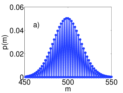
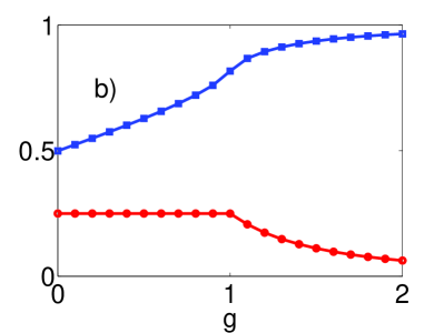
Figure 1: a) Counting probability distribution $p(m)$ of finding $m$ particles as a function of $m$ for the fermionic system Eq.(LABEL:eq-ham1) with $\gamma=\kappa$=1 and $g=0$, $N=1000$ at $T=0$. b) Mean $\bar{m}/N$ (blue squares) and variance $\sigma^{2}/N$ (red circles) of the counting distribution as a function of the transverse field $g$ at T=0.

IV.2 Counting statistics at non-zero temperature

We now turn our discussion to the case of non-zero temperature. The effect of thermal fluctuations in the system we consider is two-folded. On the one hand, thermal fluctuations allow for breaking of superfluid fermionic pairs. On the other hand, the quantum phase transition reduces to a crossover between different regions of the phase diagram. We will show that both effects are visible in the counting distribution functions.

We consider the counting statistics at finite temperature $T$ using the canonical ensemble, $\rho=\frac{1}{Z}e^{-\beta\hat{H}}$, where $\beta=\frac{1}{k_{B}T}$, the Hamiltonian is given by Eq. (2) and the partition function $Z=\mbox{Tr}\left(e^{-\beta\sum_{k}\hat{H}_{k}}\right)$. The finite temperature $T$ determines the average number of quasiparticle excitations $\hat{d}_{k}$. In order to calculate the terms $A_{k}$ and $B_{k}$ defined in Eq. (14), we write $\rho_{k}=\frac{1}{Z_{k}}e^{-\beta\hat{H}_{k}}$ where $Z_{k}=\mbox{Tr}\left(e^{-\beta\hat{H}_{k}}\right)$ and we take the trace in the basis $\{|00\rangle|01\rangle|10\rangle|11\rangle\}$. We obtain

$$A_{k}=\frac{2\kappa}{Z_{k}}(v_{k}^{2}+{e^{-\beta E_{k}}}+e^{-2\beta E_{k}}u_{k}^{2})$$

$$B_{k}=\frac{\kappa^{2}}{Z_{k}}(v_{k}^{2}+e^{-2\beta E_{k}}u_{k}^{2})$$ (20)

$$Z_{k}=1+2{e^{-\beta E_{k}}}+{e^{-2\beta E_{k}}}$$ (21)

For a given value of the transverse field $g$, we fix the temperature and obtain the number $N_{d}=\sum_{k=1}^{N/2}N^{d}_{k}$ of fermionic excitations

$$N^{d}_{k}=\mbox{Tr}\left(\rho_{k}\hat{n}^{d}_{k}\right).$$ (22)

As explained above, we use $A_{k}$ and $B_{k}$ to obtain the recursive formula for the counting distribution.

Thermal fluctuations induce the breaking of pairs. For increasing temperature, the pairing of fermions whose binding energy is proportional to $\gamma$ in Eq. (LABEL:eq-ham1) is suppressed. This is reflected in the counting distribution in such a way that the counting probability for odd numbers of particles becomes non-zero. To illustrate this, we plot in fig. 2 the probability of counting the exemplary odd value of $m=499$ particles as a function of temperature. As temperature increases, the pairs are destroyed and we observe a transition from zero probability to a finite value. We compare a system with small interaction strength $\gamma=0.01$ (fig. 2 a ) to the case of $\gamma=1$ (fig. 2 b ). In the insets, we compare the counting distribution for each system at zero temperature and at higher temperatures. We observe that the splitting between even and odd particle numbers disappears as the temperature increases. Note that here we consider a perfect detection process. For lower detection efficiency, the splitting is not visible, as was shown in Ref. counting . For small interaction strength $\gamma$, the counting distribution is narrower, while higher binding energies $\gamma$ imply broader atom number distribution functions. Also, observing the scales of temperatures when the counting of odd particles become non-zero, one can infer that this temperature is proportional to the parameter $\gamma$.

Let us now turn our discussion to the influence of temperature on the criticality of the system. As was seen above for the case of zero temperature, the phase transition is visible in the mean and variance of the distribution. This behavior is even more evident in the derivatives of the mean and variance. In fig. 3, we plot the derivative of the means and variances with respect to g at different temperatures $T$. One can see how the criticality is blurred when the temperature is of the order of the energies of the system $k_{B}T\sim E_{k}$. At high temperature, the mean and variance become independent of the transverse field value $g$ and take a constant value of $0.5N$ and $0.25N$, respectively.

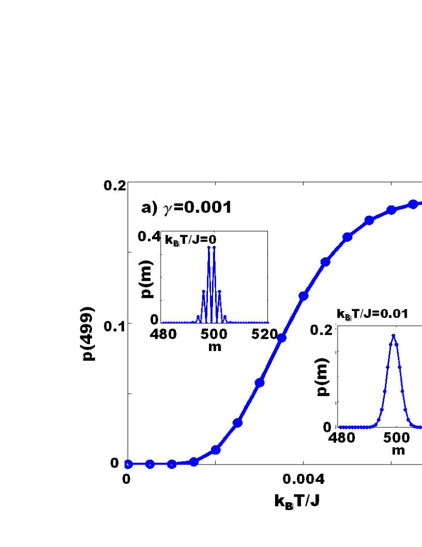
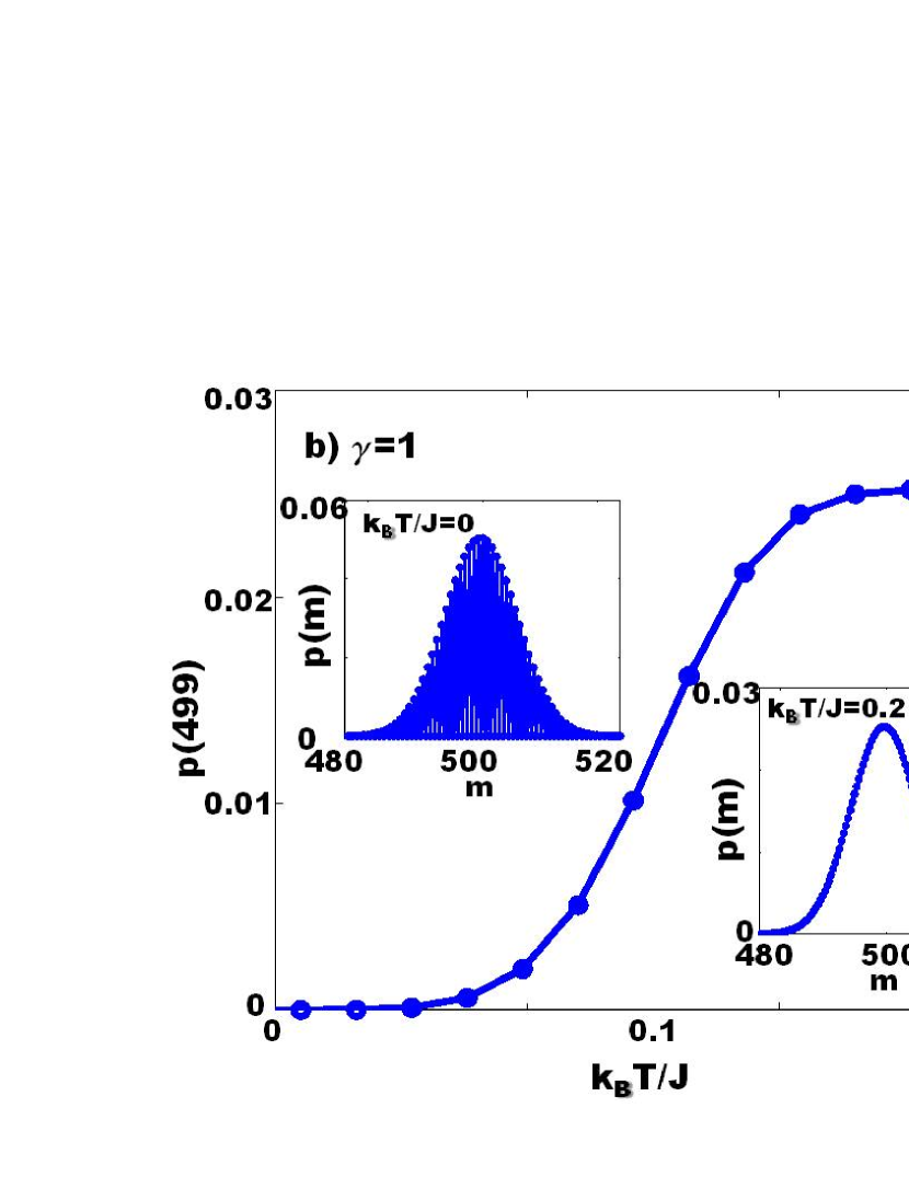
Figure 2: Probability of counting an odd number (m=499) of particles as a function of T for $\gamma=0.01$ (fig. a) and $\gamma=1$ (fig. b). The insets show the counting distribution for $T=0$ and $k_{B}T/J=0.01$ in fig. a) and for $T=0$ and $k_{B}T/J=0.2$ in fig. b).

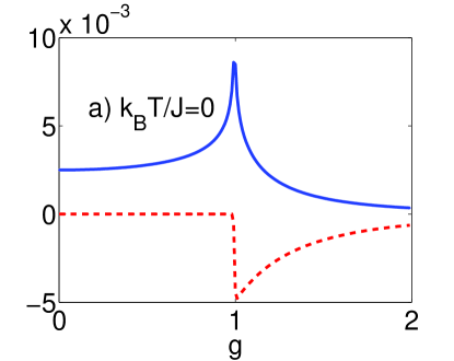
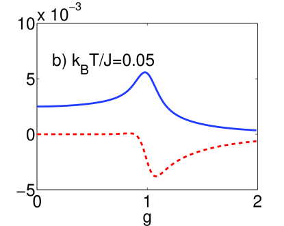
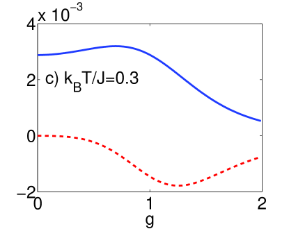
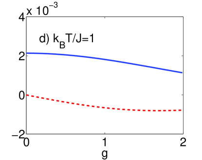
Figure 3: Derivative of the mean $\bar{m}/N$ (blue solid line) and the variance $\sigma^{2}/N$ (red dashed line) of the counting distribution of the fermionic system Eq.(LABEL:eq-ham1) with $\gamma=1$ as a function of the transverse field $g$. a) $T=0$, $N_{d}=0$ for all $g$; b) $k_{B}T/J=0.05$ and $N_{d}/N\simeq 0$ at $g=0$; c) $k_{B}T/J=0.3$ and $N_{d}/N=0.03$ at $g=0$; d) $k_{B}T/J=1$ and $N_{d}/N=0.27$ at $g=0$.

V Counting statistics during thermalization of a system coupled to a heat bath

The long decoherence times of experiments with ultracold atoms allow to study the real time quantum dynamics of the system. The dynamics of an open system coupled to a heat bath has recently aroused much interest env as one can use dissipation for quantum state engineering. By tuning the properties of the reservoir, thermalization can drive the system to a steady state which has the desired properties and can e.g. be used to encode quantum information. Here, we consider the thermalization of the system hamiltonian Eq. (LABEL:eq-ham1), when it is coupled to a heat bath. We start from the ground state at $T=0$ and let the system evolve to the thermal Boltzmann-Gibbs equilibrium state. In this sense, we analyze the counting statistics in a temperature quench. Coupling to the heat bath is described by the quantum master equation breuer

$$\frac{d}{dt}\rho(t)=$$

$$\gamma_{0}\sum_{k}(\frac{N^{d}_{k}}{2}+1)\left[\hat{d}_{k}\rho(t)\hat{d}_{k}^{\dagger}-\frac{1}{2}\hat{d}_{k}^{\dagger}\hat{d}_{k}\rho(t)-\frac{1}{2}\rho(t)\hat{d}_{k}^{\dagger}\hat{d}_{k}\right]$$

$$+\gamma_{0}\sum_{k}\frac{N^{d}_{k}}{2}\left[\hat{d}_{k}^{\dagger}\rho(t)\hat{d}_{k}-\frac{1}{2}\hat{d}_{k}\hat{d}_{k}^{\dagger}\rho(t)-\frac{1}{2}\rho(t)\hat{d}_{k}\hat{d}_{k}^{\dagger}\right],$$ (23)

where $\gamma_{0}$ is the coupling strength and $N^{d}_{k}$ defined in Eq. (22), accounts for the mean number of fermions in the mode $k$ at a certain temperature $T$. This open system dynamics assures that the system approaches thermal equilibrium towards the Boltzmann-Gibbs state.

At this point, we would like to clarify an important point in relation to particle counting of a dynamical system. The system is governed by two different dynamic processes, one is the coupling to the heat bath described by Eq. (23), the other one is the detection by particle counting described by Eq. (33) in the Appendix. We assume that the coupling of the system to the heat bath occurs on a time scale much slower than the counting process. The counting is thus performed in a time interval in which the coupling to the bath does not affect the system, so that it can be considered time independent. Below we show how the counting statistics change during thermalization of the system with the heat bath. However, each of the distributions is registered at the detector in a time interval in which no change occurs.

V.1 Coupling to the excitations

In order to calculate the counting statistics of the system coupled to a heat bath, we calculate the terms $A_{k}$ and $B_{k}$ as given in Eq. (14), which now depend on time. From the master equation (23), the time dependent mean excitation number is obtained as

$$\langle\hat{n}_{k}^{d}(t)\rangle=\hbox{e}^{-\gamma_{0}t}\langle\hat{n}_{k}^{d}(0)\rangle+N^{d}_{k}(1-\hbox{e}^{-\gamma_{0}t}).$$ (24)

We start with the system initially in the vacuum state and use

$$\langle\hat{d}_{k}^{\dagger}\hat{d}_{k}\hat{d}_{-k}^{\dagger}\hat{d}_{-k}(t)\rangle=\langle\hat{d}_{k}^{\dagger}\hat{d}_{k}\rangle_{t}\langle\hat{d}_{-k}^{\dagger}\hat{d}_{-k}\rangle_{t},$$ (25)

to calculate the time dependent terms $A_{k}(t)$ and $B_{k}(t)$ for a system in a heat bath

$$\frac{A_{k}(t)}{\kappa}=u_{k}^{2}N^{d}_{k}(1-e^{-\gamma_{0}t})+v_{k}^{2}(2-N^{d}_{k}(1-e^{-\gamma_{0}t})),$$

$$\frac{B_{k}(t)}{\kappa^{2}}=u_{k}^{2}\frac{(N_{k}^{d}(1-e^{-\gamma_{0}t}))^{2}}{4}$$

$$+v_{k}^{2}(1-N_{k}^{d}(1-e^{-\gamma_{0}t})+\frac{(N_{k}^{d}(1-e^{-\gamma_{0}t}))^{2}}{4}).$$ (26)

In fig. 4, we plot the derivatives of the mean and variance with respect to the transverse field $g$ at different times $t$ at a fixed coupling rate $\gamma_{0}=1$ and at fixed temperature of the bath $k_{B}T/J=0.1$. At the initial time $t=0$, the mean and variance correspond to those of the zero excitation state, ground state at zero temperature (fig. 4 a ). The phase transition is clearly visible in the derivative both of the mean and the variance. Due to the coupling of the system and the bath, already for intermediate times (see fig. 4 b ), the characteristic behavior of the mean and variance in the critical region washes out. For long coupling time, as shown in fig. 4 c , the behavior is completely determined by the bath.

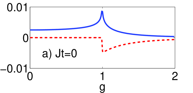
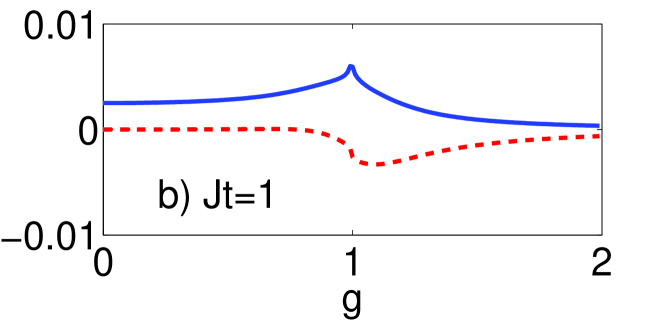
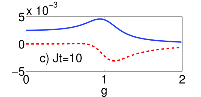
Figure 4: Thermalization: Derivative with respect to the parameter $g$ of the mean (blue solid line) and variance (red dashed line) for $\gamma=1$ for increasing coupling time with $\gamma_{0}$=1 and $k_{B}T/J=0.1$. Fig. a) shows the initial time when the system is not coupled to the bath. Fig. b) $Jt=1$ and c)$Jt=10$.

In fig. 5, we plot the mean and variance as a function of time $t$ for a system coupled to a heat bath at very high temperature $k_{B}T/J=100$. Here, the transverse field $g$ is fixed. For no transverse field $g=0$ (fig. 5 a ), both the mean and the variance are constant as the coupling increases. In the critical point $g=1$ (fig. 5 b ), the variance is constant and the mean decreases as the coupling time increases. For high transverse field $g=2$ (fig. 5 c), the mean decreases until reaching the value of $0.5N$ and the variance increases up to the value $0.25N$.

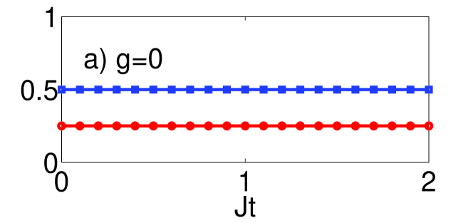
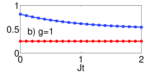
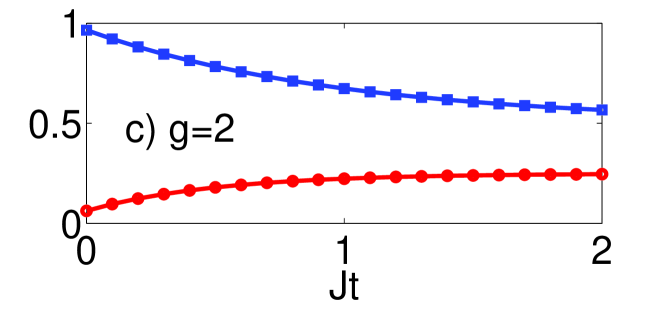
Figure 5: Thermalization: Mean (blue squares) $\bar{m}/N$ and variance $\sigma^{2}/N$ (red circles) for increasing coupling time $t$ ($\gamma=\gamma_{0}=1$). a) $g=0$, b) $g=1$ and c) $g=2$.

V.2 Local representation of the coupling

The master equation Eq. (23) that we use to describe thermalization shows two aspects. On the one hand, it is physical to describe the coupling to the bath in terms of an exchange of quasiparticles $\hat{d}_{k}$, because the Hamiltonian Eq.(LABEL:eq-ham1) conserves the number of quasiparticle excitations. On the other hand, it may look non-physical because the exchange between the system and the bath is non-local. The aim of this section is to show that the master equation can be rewritten in terms of local fermions $\hat{c}_{l}$ and in principle it could be realized using reservoir designs env .

At high temperatures and in the absence of a transverse field ($g=0$) at any temperature, the number of excitations $N_{k}^{d}$ in the bath is constant with $k$. In this case, the master equation (23) in terms of the local operators $\hat{c}_{l}$ reads

$$\frac{d}{dt}\rho(t)=$$

$$\gamma_{0}(\frac{N_{d}}{N}+1)\sum_{l,m}[F_{u}(l-m)\hat{c}_{l}\rho\hat{c}_{m}^{\dagger}+F_{v}(l-m)\hat{c}_{l}^{\dagger}\rho\hat{c}_{m}-F_{uv}(l-m)(\hat{c}_{l}^{\dagger}\rho\hat{c}_{m}^{\dagger}-\hat{c}_{l}\rho\hat{c}_{m})$$

$$-\frac{1}{2}(F_{u}(l-m)\hat{c}_{l}^{\dagger}\hat{c}_{m}\rho+F_{v}(l-m)\hat{c}_{l}\hat{c}_{m}^{\dagger}\rho-F_{uv}(l-m)(\hat{c}_{l}^{\dagger}\hat{c}_{m}^{\dagger}\rho-\hat{c}_{l}\hat{c}_{m}\rho))$$

$$-\frac{1}{2}(F_{u}(l-m)\rho\hat{c}_{l}^{\dagger}\hat{c}_{m}+F_{v}(l-m)\rho\hat{c}_{l}\hat{c}_{m}^{\dagger}-F_{uv}(l-m)(\rho\hat{c}_{l}^{\dagger}\hat{c}_{m}^{\dagger}-\rho\hat{c}_{l}\hat{c}_{m}))]$$

$$+\gamma_{0}\sum_{k}\frac{N_{d}}{N}\sum_{l,m}[F_{u}(l-m)\hat{c}_{l}^{\dagger}\rho\hat{c}_{m}+F_{v}(l-m)\hat{c}_{l}\rho\hat{c}_{m}^{\dagger}-F_{uv}(l-m)(\hat{c}_{l}^{\dagger}\rho\hat{c}_{m}^{\dagger}-\hat{c}_{l}\rho\hat{c}_{m})$$

$$-\frac{1}{2}(F_{u}(l-m)\hat{c}_{l}\hat{c}_{m}^{\dagger}\rho+F_{v}(l-m)\hat{c}_{l}^{\dagger}\hat{c}_{m}\rho-F_{uv}(l-m)(\hat{c}_{l}^{\dagger}\hat{c}_{m}^{\dagger}\rho-\hat{c}_{l}\hat{c}_{m}\rho))$$

$$-\frac{1}{2}(F_{u}(l-m)\rho\hat{c}_{l}\hat{c}_{m}^{\dagger}+F_{v}(l-m)\rho\hat{c}_{l}^{\dagger}\hat{c}_{m}-F_{uv}(l-m)(\rho\hat{c}_{l}^{\dagger}\hat{c}_{m}^{\dagger}-\rho\hat{c}_{l}\hat{c}_{m}))],$$ (27)

where we define the functions

$$F_{u}(l-m)=\frac{1}{N}\sum_{k}u_{k}^{2}e^{i\Phi_{k}(l-m)}$$ (28)

$$F_{v}(l-m)=\frac{1}{N}\ \sum_{k}v_{k}^{2}e^{i\Phi_{k}(l-m)}$$ (29)

$$F_{uv}(l-m)=\frac{i}{N}\sum_{k}u_{k}v_{k}e^{i\Phi_{k}(l-m)},$$ (30)

which depend on the distance $l-m$ between two sites $l$ and $m$ and are related to the correlation length of the quasiparticles and the pairs. In fig. 6 and fig. 7, we study the behavior of the functions $F_{u}$, $F_{v}$ and $F_{uv}$ as the distance between the sites increases. We plot $F_{u}$, $F_{v}$ and $\frac{1}{i}F_{uv}$ for different values of $g$ and $\gamma/J$ and show that the functions $F_{u}$, $F_{v}$ have their maximum at zero distance and decay rapidly as the distance increases. The function $F_{uv}$, which corresponds to the pair correlations, has its maximum at the nearest neighbor term $l-m=1$. We observe that for large transverse field $g\gg 1$, and $\gamma/J\rightarrow 0$, the only non-zero term corresponds to $F_{v}(0)=1$. In this case, the XY model behaves like a free fermi gas and the master equation (23) reduces to

$$\frac{d}{dt}\rho(t)=$$

$$\gamma_{0}(N_{d}/N+1)\sum_{l}[\hat{c}_{l}^{\dagger}\rho\hat{c}_{l}-\frac{1}{2}\hat{c}_{l}\hat{c}_{l}^{\dagger}\rho-\frac{1}{2}\rho\hat{c}_{l}\hat{c}_{l}^{\dagger}]$$

$$+\gamma_{0}N_{d}/N\sum_{l}[\hat{c}_{l}\rho\hat{c}_{l}^{\dagger}-\frac{1}{2}\hat{c}_{l}^{\dagger}\hat{c}_{l}\rho-\frac{1}{2}\rho\hat{c}_{l}^{\dagger}\hat{c}_{l}].$$ (32)

Note that for these parameters, the quasiparticles $\hat{d}_{k}\rightarrow\hat{c}_{k}^{\dagger}$. Thus at high $T$ and high transverse field $g$ the bath and the system exchange fermionic particles.

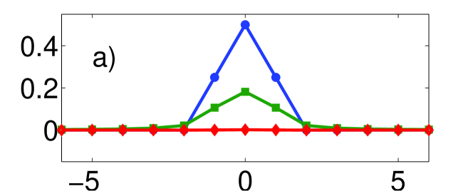
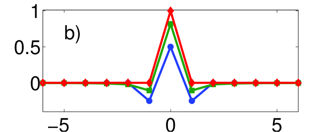
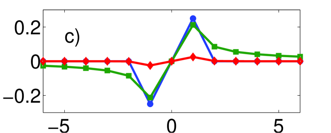
Figure 6: Thermalization: $F_{u}$ a), $F_{v}$ b) and $F_{uv}$ c) as a function of distance between sites ($l-m$) for $\gamma=1$ and $g=0$ (blue line/circles), $g=1$ (green line/squares) and $g=10$ (red line/diamands).

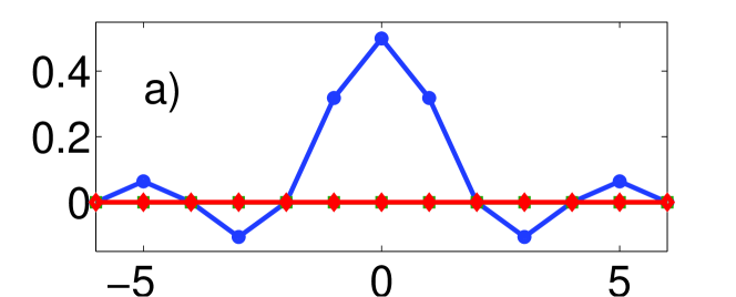
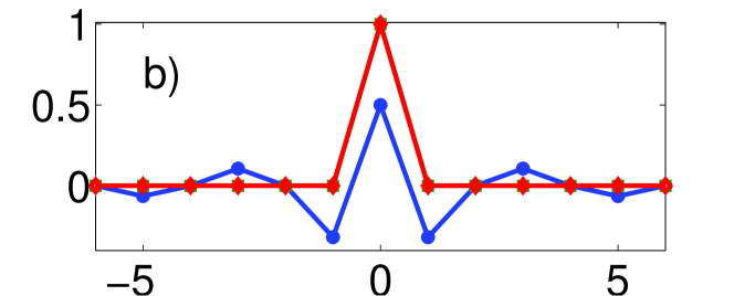
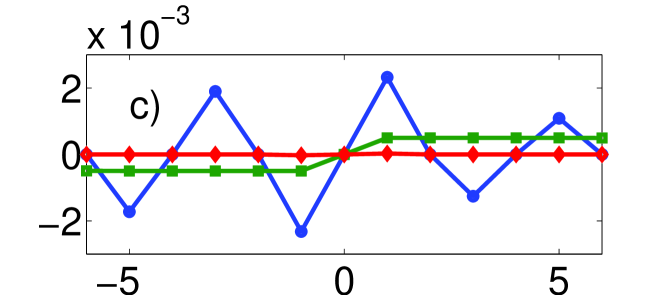
Figure 7: Thermalization: $F_{u}$ a), $F_{v}$ b) and $F_{uv}$ c) as a function of distance between sites $l-m$ for $\gamma=0.01$ and $g=0$ (blue line/circles), $g=1$ (green line/squares) and $g=10$ (red line/diamands).

Another interesting limit occurs at any $T$ when $g\rightarrow 0$ and $\gamma/J=1$. We see in figure 6 that in this case, the functions $F_{u}$, $F_{v}$ are of order $0.5$ for the same site and $F_{u}$, $F_{v}$ and $F_{uv}$ are of the order of $\pm 0.25$ for neighboring sites. The master equation Eq. (27) has contributions from exchange of on-site fermions and an additional term that corresponds to neighboring particles. Also, there is exchange of not only on-site particles and holes but also fermionic pairs. This is expected as in this regime $g\ll\gamma,J$ the pair creation dominates in Hamiltonian Eq. (LABEL:eq-ham1).

For low temperatures and at $g\neq 0$, the number of quasiparticles $N_{k}^{d}$ is not constant with $k$ and the master equation cannot be written in the form Eq. (27). However, as $N_{k}^{d}$ is small for low temperatures, the non-local terms are negligible and the equation as a whole remains local.

VI Conclusions

We have studied the effect of temperature in the counting distribution of a strongly correlated fermionic system which can be mapped to the quantum XY spin model with a transverse field. Thermal fluctuations induce pair breaking in the superfluid fermionic system. We show that this is reflected in the number distribution function which becomes non-zero for odd number of particles for a temperature proportional to the pair formation strength. Also, thermal fluctuations reduce the quantum phase transition into a crossover between different regions of the phase diagram. We have found that at low temperatures, the mean and variance of the counting distribution reflect the critical behavior at the crossover between different phase regimes. This effect is obscured with increasing temperature and when the temperature is comparable to the eigenergies of the system, the critical behavior is blurred from the cumulants of the counting distribution.

Furthermore, we have shown that the number distribution functions can be used to monitor the quantum dynamics of the system. We have studied the thermalization of the system initially at zero temperature when it is coupled to a heat bath at finite temperature. This process is analogous to a temperature quench. The temperature determines the number of delocalized excitations in the system at equilibrium. For high temperatures and high transverse fields, the exchange of excitations between system and bath can be mapped into the exchange of local fermions. For zero transverse field, we have shown that the exchange of local excitations corresponds to the exchange of local particles and nearest neighbor pairs. We have assumed that the counting process occurs at a different time scale, much faster than the exchange of excitations between the system and the bath. We have shown that the mean and variance of the counting distribution can be used to map the thermalization process.

Appendix: Counting of constant fields

The counting formula in Eq. (10) has been derived in different ways Glauber-seminal ; Mandel ; Kelley ; lax ; mollow ; scully ; selloni ; srinivas . Here, we review a derivation (see e.g. Ueda1990 ) by modeling the absorption of the particles at the detector with the master equation

$$\dot{\rho}=\varepsilon\hat{a}\rho\hat{a}^{\dagger}-\frac{\varepsilon}{2}\hat{a}^{\dagger}\hat{a}\rho-\frac{\varepsilon}{2}\rho\hat{a}^{\dagger}\hat{a},$$ (33)

where $a^{\dagger}$ and $a$ are the creation and annihilation operator of the particle to be counted. Performing a rotation of the density matrix, $\rho(t)=e^{-\frac{\varepsilon}{2}t\hat{a}^{\dagger}\hat{a}}\tilde{\rho}(t)e^{-\frac{\varepsilon}{2}t\hat{a}^{\dagger}\hat{a}}$, and using the relation

$$e^{\gamma A}Be^{-\gamma A}=B+\gamma[A,B]+\frac{\gamma^{2}}{2!}[A,[A,B]]+...,$$ (34)

we obtain

$$\dot{\tilde{\rho}}(t)=\varepsilon\hat{a}e^{\frac{-\varepsilon}{2}t}\tilde{\rho}\hat{a}^{\dagger}e^{\frac{-\varepsilon}{2}t}=\varepsilon e^{-\varepsilon t}\hat{a}\tilde{\rho}\hat{a}^{\dagger}.$$ (35)

This equation can be solved using perturbation theory

$$\tilde{\rho}(t)=\tilde{\rho}(0)+\int_{0}^{t}\varepsilon e^{-\varepsilon t^{\prime}}\hat{a}\tilde{\rho}(t^{\prime})\hat{a}^{\dagger}.$$

Transforming back the rotation we obtain

$$\rho(t)=e^{-\frac{\varepsilon}{2}t\hat{a}^{\dagger}\hat{a}}(\tilde{\rho}(0)+\int_{0}^{t}\varepsilon e^{-\varepsilon t^{\prime}}\hat{a}\tilde{\rho}(0)\hat{a}^{\dagger}+...)e^{-\frac{\varepsilon}{2}t\hat{a}^{\dagger}\hat{a}}.$$ (37)

Using the cyclic properties of the trace, the probability $p_{m}(t)$ of counting $m$ particles can be written as

$$p_{m}(t)=\hbox{Tr}[\rho(0)a^{{\dagger}m}\frac{(\int_{0}^{t}dt^{\prime}\varepsilon e^{-\varepsilon t^{\prime}})^{m}}{m!}e^{-\varepsilon ta^{\dagger}a}a^{m}].$$ (38)

This is equal to the normally ordered expression

$$p_{m}(t)=\langle:(1-e^{-\varepsilon t})^{m}\frac{(\hat{a}^{\dagger}\hat{a})^{m}}{m!}e^{-(1-e^{-\varepsilon t})\hat{a}^{\dagger}\hat{a}}:\rangle,$$ (39)

which holds because

$$:(\hat{a}^{\dagger}\hat{a})^{m}e^{-(1-e^{-\varepsilon t})\hat{a}^{\dagger}\hat{a}}:=\hat{a}^{{\dagger}m}:e^{-(1-e^{-\varepsilon t})\hat{a}^{\dagger}\hat{a}}:\hat{a}^{m}$$

$$=\hat{a}^{{\dagger}m}e^{-\varepsilon t\hat{a}^{\dagger}\hat{a}}\hat{a}^{m}.$$ (40)

We can thus use the generating function formalism in Eq.(12) with $\kappa=\int_{0}^{\tau}dt^{\prime}\varepsilon e^{-\varepsilon t^{\prime}}=1-\exp{(-\varepsilon\tau)}$, where $\tau$ is the aperture time of the detector.

- (1) M. Lewenstein, A. Sanpera, V. Ahufinger, B. Damski, A. Sen(De), and U. Sen, Adv. Phys., 56, 243 (2007).
- (2) S. Trotzky, P. Cheinet, S. Fölling, M. Feld, U. Schnorrberger, A. M. Rey, A. Polkovnikov, E. Demler, M. D. Lukin, and I. Bloch, Science 319, 295 (2008).
- (3) K. Jiménez-García, R. L. Compton, Y.-J. Lin, W. D. Phillips, J. V. Porto, and I. B. Spielman, cond-mat/1003.1541.
- (4) G.B. Jo, Y.R. Lee, J.H. Choi, C.A. Christensen, T.H. Kim, J.H. Thywissen, D.E. Pritchard, and W. Ketterle, Science 325 , 1521 (2009).
- (5) K. Sengupta, S. Powell, S. Sachdev, Phys. Rev. A 69, 053616 (2004).
- (6) J. Eisert, M. B. Plenio, S. Bose and J. Hartley, Phys. Rev. Lett. 93, 190402 (2004); A. Sen (De), U. Sen and M. Lewenstein, Phys. Rev. A 70, 060304 (2004); ibid 72, 052319 (2005).
- (7) S. R. Manmana, S. Wessel, R. M. Noack, and A. Muramatsu, Phys. Rev. Lett. 98, 210405 (2007).
- (8) M. Cramer, A. Flesch, I. P. McCulloch, U. Schollw ck, and J. Eisert, Phys. Rev. Lett. 101, 063001 (2008).
- (9) S. Deng, G. Ortiz and L. Viola, Phys. Rev. B 80, 241109 (R) (2010).
- (10) M. C. Ba uls, J. I. Cirac, M. B. Hastings, arXiv:1007.3957 (2010).
- (11) B. Kraus, H. P. Büchler, S. Diehl, A. Kantian, A. Micheli, and P. Zoller, Phys. Rev. A 78 042307 (2008); S. Diehl, A. Micheli, A. Kantian, B. Kraus, H. P. Büchler, and P. Zoller, Nat. Phys. 4 878 (2008); F. Verstraete , M. M. Wolf, and J. I. Cirac, Nat. Phys. 5 633 (2009).
- (12) R. J. Glauber, Phys. Rev. 130 2529 (1963), R.J. Glauber Phys. Rev. 131 2766 (1963), R.J. Glauber, in Quantum Optics and Electronics, eds. B. DeWitt, C. Blandin, and C. Cohen-Tannoudji, pp. 63-185 (Gordon and Breach, New York, 1965).
- (13) F. Hassler, M. V. Suslov, G. M. Graf, M. V. Lebedev, G. B. Lesovik, and G. Blatter, Phys. Rev. B 78, 165330 (2008).
- (14) A. Bednorz, W. Belzig, Phys. Rev. B 81, 125112 (2010).
- (15) W. Belzig, and Y. V. Nazarov, Phys. Rev. Lett. 87 197006 (2001).
- (16) J. Börlin, W. Belzig, and C. Bruder, Phys. Rev. Lett. 88, 197001 (2002).
- (17) T. Karzig, and F. von Oppen, Rhys. Rev. B 81 045317 (2010).
- (18) L. S. Levitov, H. Lee, and G. B. Lesovik, J. Math. Phys. 37, 4845 (1996); G. B. Lesovik, F. Hassler, and G. Blatter, Phys. Rev. Lett. 96, 106801 (2006); F. Hassler, G. B. Lesovik, and G. Blatter, Phys. Rev. Lett. 99 076804 (2007).
- (19) K. Schönhammer, J. Phys.: Condens. Matter 21 495306 (2009).
- (20) S. Sachdev, Quantum Phase Transitions (Cambridge University Press, Cambridge, 2001).
- (21) R. W. Cherng and E. Demler, New J. Phys. 9, 7 (2007).
- (22) W. Belzig, C. Schroll, and C. Bruder, Phys. Rev. A 75, 063611 (2007).
- (23) M. Lewenstein, Nature 445, 372 (2007).
- (24) S. Braungardt, A. Sen(De), U. Sen, R. J. Glauber, and M. Lewenstein, Phys. Rev. A 78, 063613 (2008).
- (25) S. Staudenmayer, W. Belzig, and C. Bruder, Phys. Rev. A 77, 013612 (2008).
- (26) M. Yasuda and F. Shimizu, Phys. Rev. Lett. 77, 3090 (1996).
- (27) M. Schellekens, R. Hoppeler, A. Perrin, J. Viana Gomes, D. Boiron, A. Aspect, and C.I. Westbrook, Science 310, 648 (2005), T. Jeltes, J. M. McNamara, W. Hogervorst, W. Vassen, V. Krachmalnicoff, M. Schellekens, A. Perrin, H. Chang, D. Boiron, A. Aspect, and C. I. Westbrook, Nature 445, 402 (2007).
- (28) W. S. Bakr, J. I. Gillen, A. Peng, S. Fölling and M. Greiner, Nature 462, 74 (2009).
- (29) S. Will, T. Best, U. Schneider, L. Hackermüller, D-S Lühmann and I. Bloch, Nature 465, 197 (2010).
- (30) J.L. Sorensen, J. Hald, and E.S. Polzik, Phys. Rev. Lett. 80, 3847 (1998).
- (31) K. Eckert, O. Romero-Isart, M. Rodriguez, M. Lewenstein, E.S. Polzik, and A. Sanpera, Nature Physics 4, 50 - 54 (2008).
- (32) T. Roscilde, M. Rodriguez, K. Eckert, O. Romero-Isart, M. Lewenstein, E. Polzik, A. Sanpera, New J. Phys. 11, 055041 (2009).
- (33) R. Jördens, N. Strohmaier, K. Günter, H. Moritz and T. Esslinger, Nature 455, 204 (2008).
- (34) J.K. Chin, D.E. Miller, Y. Liu, C. Stan, W. Setiawan, C. Sanner, K. Xu, W. Ketterle, Nature 443, 961 (2006).
- (35) S. Katsura, Phys. Rev. 127, 1508 (1962); P. Pfeuty, Ann. Phys. (N.Y.) 57, 79 (1970); E. Lieb, T. Schultz, and D. Mattis, Ann. Phys. (N.Y.) 16, 407 (1961); E. Barouch, B.M. McCoy and M. Dresden, Phys. Rev. A 2, 1075 (1970); E. Barouch and B.M. McCoy, Phys. Rev. A 3, 786 (1971); ibid., 2137 (1971).
- (36) P. Jordan and E. Wigner, Z. Phys. 47, 631 (1928).
- (37) R.J. Glauber, in Quantum Optics and Electronics, eds. B. DeWitt, C. Blandin, and C. Cohen-Tannoudji, pp. 63-185 (Gordon and Breach, New York, 1965).
- (38) K.E. Cahill and R.J. Glauber, Phys. Rev. A 59, 1538 (1999).
- (39) H. Breuer and F. Petruccione, The Theory of Open Quantum Systems (Oxford University Press, Oxford, 2002).
- (40) L. Mandel, ECG Sudarshan, and E. Wolf, Proc. Phys. Soc. 84 135 (1964).
- (41) P. L. Kelley, and W. H. Kleiner, Phys. Rev. A 136 316 (1964).
- (42) M. Lax, and M. Zwanziger, Phys. Rev. A 136 316 (1964).
- (43) B. R. Mollow, Phys. Rev. 168, 1896 (1968).
- (44) M. O. Scully, and W. E. Lamb, Jr., Phys. Rev. 179, 368 (1969).
- (45) A. Selloni, P. Quattropani, and H. P. Baltes, J. Phys . A 11, 1427 (1978).
- (46) M. D. Srinivas, and E. B. Davies, Journal of Modern Optics 28, 7, 981-996 (1981).
- (47) M. Ueda, N. Imoto, and T. Ogawa, Phys. Rev. A 41 3891-3904 (1990).