A Wiener-Laguerre model of VIV forces given recent cylinder velocities

Abstract

Slender structures immersed in a cross flow can experience vibrations induced by vortex shedding (VIV), which cause fatigue damage and other problems. VIV models in engineering use today tend to operate in the frequency domain. A time domain model would allow to capture the chaotic nature of VIV and to model interactions with other loads and non-linearities. Such a model was developed in the present work: for each cross section, recent velocity history is compressed using Laguerre polynomials. The compressed information is used to enter an interpolation function to predict the instantaneous force, allowing to step the dynamic analysis. An offshore riser was modeled in this way: Some analyses provided an unusually fine level of realism, while in other analyses, the riser fell into an unphysical pattern of vibration. It is concluded that the concept is promissing, yet that more work is needed to understand orbit stability and related issues, in order to further progress towards an engineering tool.

1 Introduction

Vortex induced vibration (VIV) is a vibration of an elastic structure that occurs when a fluid flowing around the structure sheds vortices at near-regular intervals, locked with the structure’s own vibration. VIV is a major concern in the offshore oil industry in particular, where marine currents can cause slender structures like pipelines, risers, umbilicals and cables to vibrate, inducing fatigue damage. VIV is a hard problem because on one hand full hydrodynamic computations of vortex sheddings from structures are as yet impractical, and on the oher hand, it is challenging to simplify a strongly non-linear dynamic system. Semi empirical VIV models provide the state of the art of VIV engineering. They work by predicting added mass and excitation coefficients on the basis of reduced frequency and amplitude of vibration, and seek one or several oscillation modes that satisfy equilibrium.

Compared to such semi empirical VIV models, in the long term an efficient time-domain VIV model would open new possibilities :

1. Study of VIV on non-linear structures, for example studying the damping effect of seafloor interaction in a steel riser, or using a hysteretic cross section model for VIV on flexible pipes.

2. Accounting for VIV caused by unsteady water flows, in particular by waves or vessel motions.

3. Accounting for the increase in drag at wave frequency due to VIV.

4. Accounting for the superposition of wave-frequency and VIV-frequency stresses in fatigue analysis.

5. Accounting for the asymmetry of oscillation patterns in the vicinity of, for example, a seafloor.

The objective of the work reported here is to demonstrate the viability of a local, deterministic, time-domain force model for VIV on slender bodies with cylindric cross sections. This force model is used at each Gauss point of the dynamic finite element (FE) model of a slender structure subject to external steady or unsteady water currents, during a time domain analysis (e.g. Newmark-$\beta$ time integration with Newton-Raphson iteration). Hence the FE model resembles that commonly used in a slender structure analysis, with degrees of freedom for the structure, and none for the surrounding fluid. In other words, the proposed model takes the place usually held in software by the Morison model for wave induced loads.

The litterature describes a few time-domain models of VIV that, like the present model, do not explicitely model the wake flow. In [8], at any step and point along a cable, the recent velocity history is approximated by a harmonic function, which is then used to enter charts that predict excitation and added mass coefficients as a function of reduced amplitude and frequency. A model which could be described in the same way, but differs in several details was developped by [6]. More recently, the hydrodynamic force has been described as the response on a non-linear single degree of freedom van der Pol oscilator [4, 15, 24, 25]. The models enumerated here only deal with cross-flow vibration.

The present model differs from the above ones in that it treats in-line and cross flow vibrations jointly, does not use a harmonic simplification of the motion or forces, and does not reduce the wake response to a single degree of freedom system.

2 Model outline

2.1 Postulate

The present work hinges on the following postulate. The force exerted by the surrounding fluid on a section of the slender structure, is completely determined by the recent histories at that section of the velocities of the structure and the undisturbed fluid. Several points in this sentence are worthy of discussion.

The “force” includes the components usually distributed into added mass, excitation forces, drag, lift etc… .

That the force “at section of the slender structure” is determined by the history “at that section” implies a “strip theory” in which it is excluded that motions of the structure at a point A cause disturbances in the fluid that affects the force at point B away from A. In other words, it is assumed that there is no significant transmission of information in the axial direction within the water (as opposed to within the slender structure). This would be proved wrong if it turned out that unstable phenomena, like boundary layer shedding, although transmitting little energy along the structure, transmits information that steers how local hydrodynamic energy is channeled at a given point along the structure.

That the force should be “completely determined” implies that the behavior of the structure is deterministic. This does not contradict the observation of hysteretic response of short cylinders mounted on elastic support. Uniqueness of forces given a position does not imply uniqueness of static equilibrium. Neither does “completely determined” contradict the observation of irregular and unpredictable responses to VIV: non-linear dynamic systems can have a chaotic behavior. Still, complete determinism is provably wrong, since a short vertical cylinder dragged at uniform speed through water will experience oscillating lift forces. At any given moment, there is nothing in the history of (constant) velocity that allows to predict whether the lift is left or right. So the present work is based on the bet that ignoring such “bifurcations” still leaves us with a useful model.

“History” here relates to causality. The force on the structure does not depend of future motion of the structure. By contrast, frequency-domain models do not make an explicit distinction here, typicaly requiring a steady state vibration. This can also be contrasted to Morison’s equation which predicts forces on a cylinder from instantaneous relative velocities and accelerations.

“Recent” can be defined as anything between the present time and a few times $t_{w}$, where the value of $t_{w}$ still is an object of debate. $t_{w}$ is likely to be case dependent. Current will transport (convect) away vortices so that they quickly loose significance, so that $t_{w}$ should be of the order of $D/U$ where $D$ is the cross section diameter and $U$ the current velocity. In contrast, if the cylinder is oscillating in still water, it will be traveling in its own wake, and $t_{w}$ should be related to the rate of diffusion and/or viscous dissipation of vortices, which is likely to result in much higher values of $t_{w}$. Tests on periodic forced motion of short cylinders sometimes show a slow drift of the forces (over as many as ten periods). In contrast, force decay tests for a cylinder stopped after oscilliations at zero mean velocity, point towards a fraction of a period. In the present work, the idea is to chose a “universal” value of $t_{w}$ for the system, after adequate scaling (cf. Section 3.2).

The “velocities” are what count. Accelerations would not do because for example, zero acceleration can correspond to different speeds and hence different forces. On the other hand, the force on a cylinder will not be affected by a uniform translation of its whole trajectory, so a history of positions contains irrelevant information.

In the remained of this text, the word “trajectory” will be given a very specific meaning. The trajectory is defined as the recent history of the velocity vector of the cylinder relative to the undisturbed surrounding fluid.

2.2 Restrictions

In the present phase of research, the following restrictions are introduced, in order to achieve some simplification of the task. The outer cross section of the slender structure is assumed perfectly circular and smooth. The surrounding fluid is assumed to be infinite, excluding the presence of sea floor, free surface or neighbouring risers. Only fluid flows perpendicular to the cylinder at any point are considered.

2.3 Input and output

As stated earlier, the VIV model being developed herel replaces the Morison model for wave induced loads. The VIV model is called at each step and iteration, and at each Gauss point or node of each element.

The model is to receive as input:

1. the diameter of the cylinder.

2. the instantaneous velocity of the cross section relative to the undisturbed fluid.

3. the instantaneous velocity and acceleration of the local undisturbed fluid, in a Galilean reference system.

The model uses velocity information stored from previous steps. On this basis, the model produces as output:

1. the vector of hydrodynamic forces per unit length, acting on the cylinder.

2. the matrix containing the derivative of the above with respect to instantaneous values of the cylinder’s behaviour.

Gauss integration is then used to compute a consistent load vector and derivative matrix for each element. Note that these element matrices are likely to vary significantly over each VIV oscillation “period” - in contrast to added mass or damping matrices, deemed to be constant over a long time in semi-empirical VIV models. The connection of the force model to the finite element analysis is discussed in Section 7.

2.4 Algorithmic steps

Only the local VIV model is described here, not the whole FE analysis.

1. The relative velocity of the cylinder relative to water (thereafter: “velocity”) is computed.

2. The velocity is scaled (Reynolds scaling) to that the cylinder diameter is the unit of distance (Section 3.2).

3. The trajectory (again: the recent histories of both $x$ and $y$ components of velocity) is compressed to a small number of “Laguerre coefficients”. This compression is such that it provides accurate information over the recent past and increasingly coarse information for more distant past (Section 4).

4. The Laguerre coefficients are used to enter an interpolation function (a feed-forward neural network with some specifically tailored properties) which returns $x$ and $y$ components of hydrodynamic force (Section 5). The fitting of the interpolation function is discussed in Section 8.1.

5. The force is scaled back to the relevant diameter (Section 3.2)

6. The Froude-Krylov forces, which depend on the acceleration of the undisturbed flow, are added (Section 3.1)

The identification of non-linear systems using a bank of orthogonal filters (including Laguerre filter) to generate multiple signals from a single one, and then using the multiple signals to enter a non-linear, memory-less function, was introduced by Norbert Wiener [26]. In the present work, a base of Laguerre polynomials is used, in contrast to Laguerre functions introduced by Wiener. While Wiener apparently did not use neural networks as non-linear functions (but for example Hermite polynomials), neural networks in Wiener models have been studied for some time [2]. In the present work, Laguerre filtering is presented without making use of the vocabulary of cybernetics. In particular, the $z$-transform is not introduced here.

3 Ancillary transformations

3.1 Froude-Krylov forces

This section gives the justification for point 6 of Section 2.4. If the undisturbed fluid in which the cylinder is plunged is accelerating (because of surface waves, for example), then it is natural to introduce two reference systems: $\mathfrak{G}$ is a Galilean reference system, for example fixed relative to the sea floor, $\mathfrak{A}$ is an accelerated reference system, locally following the undisturbed flow. Transforming the equations of equilibrium from $\mathfrak{G}$ (in which we carry out FEM analysis) to $\mathfrak{A}$ (for which we have experimental data, in water that is no accelerated) requires the addition of inertia forces.

The inertial forces create a uniform pressure gradient that was not present in the laboratory test. The effect of a pressure gradient on a submerged body is variously referred to as “Archimedes forces” when the pressure gradient results from the acceleration of gravity, or as “Froude-Krylov forces” when the pressure gradient is due to fluid acceleration in surface waves. As familiar, the integral of the pressure over the wet surface is transformed into a volume integral [5].

It is assumed that this pressure gradient does not affect the turbulent flow, so that the pressure gradient can simply be added to the pressures resulting from turbulence. This seems reasonable enough for incompressible flows, and indeed when it comes to Archimedes forces, the submerged weight of a cylinder is routinely subtracted to laboratory measurements and the relevant correction added again in FEM analysis - even though the Archimedes forces in the laboratory do not necessarily scale with those in the analysis. Further there is no experimental indication that a horizontal and vertical cylinder, all other conditions being equal, experience different forces.

To conclude, the hydrodynamic force acting on the cylinder at a given instant is the sum of two terms:

1. A force that is a function of only the cylinder diameter and the recent history of the velocity of the cylinder relative to the undisturbed, steady water flow.

2. Froude-Krylov forces.

All computations in Sections 4 and 5 deal only with the first of the above two terms.

3.2 Scaling

This section details how points 2 and 5 of Section 2.4 are implemented. In order to reduce the amount of experimental data necessary to create the interpolation function used in point 4, one must take advantage of scale similarities. To that effect, all data used to either train or query the database is scaled. Correspondingly, all forces returned by the database are scaled back.

VIV forces are assumed to be uniquely defined by fluid density $\rho$, kinematic viscosity $\nu$, cylinder diameter $D$ and the motion. Hence, in order to create a database that is be entered with scaled velocities, we wish all experimental data to be scaled to fixed reference values $\rho_{o}$, $\nu_{o}$ and $D_{o}$. By expressing the units of these quantities, one gets three equations on $\lambda_{m}$, $\lambda_{s}$ and $\lambda_{kg}$, which are the scaling factors for the basic units of distance, time and mass. Solving the system yields

$$\lambda_{m} = D_{o}\frac{1}{D}$$ (1)

$$\lambda_{s} = \frac{D_{o}^{2}}{\nu_{o}}\frac{\nu}{D^{2}}$$ (2)

$$\lambda_{kg} = \rho_{o}D_{o}^{3}\frac{1}{\rho D^{3}}$$ (3)

Once the scaling of basic units is known, the scaling of any derived quantities e.g. velocities, accelerations and forces per unit length can be expressed:

$$\lambda_{ms^{-1}} = \frac{\nu_{o}}{D_{o}}\frac{D}{\nu}$$ (4)

$$\lambda_{ms^{-2}} = \frac{\nu_{o}^{2}}{D_{o}^{3}}\frac{D^{3}}{\nu^{2}}$$ (5)

$$\lambda_{Nm^{-1}} = \frac{\rho_{o}\nu_{o}^{2}}{D_{o}}\frac{D}{\rho\nu^{2}}$$ (6)

Note that since scaling is applied consistently to all derived quantities, all non-dimensional numbers based on combinations of distance, time and mass (including Reynolds and Froude numbers) is conserved. However, any dimensional quantity with units different from those of $\rho$, $\nu$ and $D$ is scaled to values that depend of $\rho$, $\nu$ and $D$. In particular, Equation 5 shows that all accelerations, including the acceleration of gravity $g$ are scaled with a factor proportional to $D^{3}/\nu^{2}$. So while the scaling used here may conserve Froude’s number, it does not allow to build a database of forces related to surface wave effects, because the database does not refer to a constant value $g_{o}$.

The choice of $\rho_{o}$, $\nu_{o}$ and $D_{o}$ is arbitrary, and in this work, all are set to the value 1. $D_{o}=1\,[m]$ implies that scaled displacements can be considered to have “1 diameter” as unit. $D_{o}=1\,[m]$ and $\nu_{o}=1\,[m^{2}/s]$ together imply that scaled velocities are expressed as Reynolds numbers since the scaled velocity is calculated as $Dv/\nu$ where $v$is the velocity.

The Reynolds number is usualy computed using some velocity characteristic of the system under study. In VIV science, the undisturbed velocity of the current is used. By contrast, in this work, instantaneous local values of the relative velocity vector is multiplied by $\frac{D}{\nu}$. The scaled velocities thus obtained are a generalisation of the traditional use of Reynolds number: Considering an immobile cylinder in a current, the norm of its scaled relative velocity vector is equal to the traditional Reynolds number. To prevent confusion of the present usage of Reynolds number with the more particular classical one, yet emphasize the relation between both, the expression “ilr-Reynolds” (for “instant, local, relative Reynolds”) will be used in this document.

4 Characterization of trajectory

4.1 Foreword

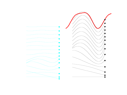
Figure 1: Weighted Laguerre polynomials (blue) are summed (black) to approximate a trajectory (red). Vertical shifts were added for readability. The

This section details how point 3 in Section 2.4 is to be implemented. The objective is, for any given point in time, to distill a “summary” of the recent history of the velocity of the cylinder relative to the surrounding fluid (trajectory). Note that the history of each component of the velocity vector is treated separately in this section and that the procedure is applied to the scaled trajectory.

The trajectory is approximated as a linear combination of some adequate family of functions, and the coefficients in this linear combination are the summary (Figure 1. The family of functions that is used here is the series of Laguerre polynomials (Section4.2). It is shown in Section 4.3 that if the “Laguerre coefficients” of the linear combination are obtained by integrating the product of the trajectory by adequate “Laguerre dual” functions, then the difference between the approximating linear combination and the real trajectory is small in the recent past and larger in the further past. This justifies the choice of Laguerre polynomials: they allow to summarise the trajectory in a way that represents recent velocities very precisely, and older velocities in a coarser manner. It is assumed that this corresponds to the information needed to obtain a good estimate of the hydrodynamic force.

Computing the integral of the product of Laguerre duals and trajectory takes time. Luckily, one can show (Section 4.5) that the Laguerre coefficients are the solution of a differential equation driven by the instant value of the velocity. To obtain results that are independent of step size, this differential equation must be carefully discretized in time (Section 4.6) when summarizing experimental data.

4.2 Definitions

The Laguerre polynomial (Figure 2, top) of degree $i-1$ can be defined by its Rodrigues formula [1]

$$\mathcal{L}_{i}\left(x\right)\equiv\frac{e^{x}}{i!}\frac{d^{i}}{dx^{i}}\left(x^{i}e^{-x}\right)$$ (7)

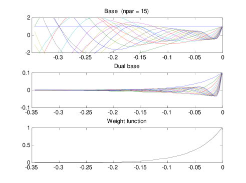
Figure 2: Laguerre polynomials (top), Laguerre duals (middle) and weight function (bottom). Taking the convolution of a signal by the Laguerre duals one obtains Laguerre coefficients. If one takes the linear combinations of the Laguerre polynomials weighted by the coefficients, one gets an approximation of the original signal, with a quality that decreses towards the past in a way related to the weight function.

Laguerre polynomials verify the orthonormality property

$$\int_{0}^{{}^{\infty}}\mathcal{L}_{i}\left(x\right)\mathcal{L}_{j}\left(x\right)e^{-x}dx=\delta_{ij}$$ (8)

We seek to describe the recent trajectory with a precision that is good for the immediate past, and decreasing for the further past. To this end, we introduce a weight function which emphasizes “recent past” (Figure 2, bottom)

$$\mathcal{W}(t)\equiv\frac{e^{\frac{t}{t_{w}}}}{t_{w}}\quad t\in\mathbb{R^{\mathrm{-}}}$$ (9)

were the interpretation of $t_{w}$ has been discussed in Section 2.1. Functions will now be noted as vectors (in a Hilbert space), marked with overlined symbols. An indexed family of functions will be noted as a matrix (symbols with double overline) and so will a linear operator (a distributions of two variables). We introduce the symmetric positive definite operator

$$\overline{\overline{W}}(t_{1},t_{2})=\delta(t_{1},t_{2})\mathcal{W}(t_{1})$$ (10)

and a dot product in a suitable space of real valued functions

$$\overline{f}^{T}\circ\overline{g}\equiv\intop_{-\infty}^{0}f(t)g(t)dt$$ (11)

with the canonical norm

$$\left|\overline{f}\right|\equiv\sqrt{\overline{f}\circ\overline{f}}$$ (12)

Further we introduce the base

$$\overline{\overline{L}}(t,i)\equiv\mathit{\mathcal{L}}_{i}(-t/t_{w})\quad t\in\mathbb{R^{\mathrm{-}}},\>i\in\left\{1,\ldots,n\right\}$$ (13)

Equation 8 can be rewritten in matrix notation as

$$\overline{\overline{I}}=\overline{\overline{L}}^{T}\circ\overline{\overline{W}}\circ\overline{\overline{L}}$$ (14)

where $\bar{\bar{I}}$ is the $n\times n$ identity matrix. It is useful to introduce the weighted norm or $w$-norm

$$\left|\overline{f}\right|_{w}\equiv\sqrt{\overline{f}\circ\overline{\overline{W}}\circ\overline{f}}$$ (15)

Note that since $\mathcal{W}(t)$ is of dimension $[1/s],$ $\left|\overline{f}\right|_{w}$ is of the same dimension as$\overline{f}$. So went taking $\overline{f}$ as a scaled velocity, $\left|\overline{f}\right|_{w}$ is an ilr-Reynolds number.

4.3 Analysis and synthesis

For a history $\overline{v}(t)$ of either the $x$ or $y$ component of the velocity, we seek the vector of “Laguerre coefficients” $\overline{\tau}$ for the above base that minimize the weighted discretization error

$$J = \frac{1}{2}\left|\overline{v}-\overline{\overline{L}}\cdot\overline{\tau}\right|_{w}^{2}$$ (16)

$$= \frac{1}{2}\left(\overline{v}-\overline{\overline{L}}\cdot\overline{\tau}\right)^{T}\circ\overline{\overline{W}}\circ\left(\overline{v}-\overline{\overline{L}}\cdot\overline{\tau}\right)$$ (17)

To this effect we require that the derivative be zero:

$$\frac{\partial J}{\partial\overline{\tau}}=\overline{\overline{L}}^{T}\circ\overline{\overline{W}}\circ\overline{\overline{L}}\cdot\overline{\tau}-\overline{\overline{L}}^{T}\circ\overline{\overline{W}}\circ\overline{v}$$ (18)

which implies

$$\overline{\tau} = \left(\overline{\overline{L}}^{T}\circ\overline{\overline{W}}\circ\overline{\overline{L}}\right)^{-1}\cdot\overline{\overline{L}}^{T}\circ\overline{\overline{W}}\circ\overline{v}$$ (19)

$$= \overline{\overline{L}}^{T}\circ\overline{\overline{W}}\circ\overline{v}$$ (20)

$$\overline{\tau} = \overline{\overline{D}}^{T}\circ\overline{v}$$ (21)

with

$$\overline{\overline{D}}\equiv\overline{\overline{W}}\circ\overline{\overline{L}}$$ (22)

where the functions $\overline{\overline{D}}$ used for analysis consists of the Laguerre duals (Figure 2, middle. Not to be confused with the Laguerre functions introduced in Equation 27)

$$\overline{\overline{D}}(t,i) = \mathcal{D}_{i}(-t/t_{w})$$ (23)

$$= \mathcal{L}_{i}(-t/t_{w})\frac{e^{\frac{t}{t_{w}}}}{t_{w}}$$ (24)

Although

$$\overline{\overline{D}}^{T}\circ\overline{\overline{L}}=\overline{\overline{I}}$$ (25)

the functions in $\overline{\overline{D}}$ and $\overline{\overline{L}}$ do not span the same space. Hence the appellation “dual base” is abusive.

4.4 Convergence

Laguerre functions, which can be defined as

$$\overline{\overline{F}}\left(t,i\right) \equiv \mathcal{F}_{i}(-t/t_{w})$$ (26)

$$\equiv \mathcal{L}_{i}(-t/t_{w})\frac{e^{\frac{t}{2\>t_{w}}}}{2t_{w}}$$ (27)

or, in matrix notation

$$\overline{\overline{F}}=\sqrt{\overline{\overline{W}}}\circ\overline{\overline{L}}$$ (28)

have been extensively studied. Series of Laguerre functions are known to converge almost everywhere (under some conditions of continuity) [18]. In matrix notation this result can be stated as

$$\lim_{n\rightarrow\infty}\left|\overline{\overline{F}}\cdot\overline{\overline{F}}^{T}\circ\overline{f}-\overline{f}\right|=0$$ (29)

This can be used to obtain a result on the convergence of series of Laguerre polynomials. We introduce the change of variables

$$\overline{f}=\sqrt{\overline{\overline{W}}}\circ\overline{g}$$ (30)

so that

$$\left|\overline{\overline{F}}\cdot\overline{\overline{F}}^{T}\circ\overline{f}-\overline{f}\right| = \!\!\!\!\left|\overline{\overline{F}}\cdot\overline{\overline{D}}^{T}\circ\overline{g}-\sqrt{\overline{\overline{W}}}\circ\overline{g}\right|$$ (31)

$$= \!\!\!\!\left|\sqrt{\overline{\overline{W}}}\circ\left(\overline{\overline{L}}\cdot\overline{\overline{D}}^{T}\circ\overline{g}-\overline{g}\right)\right|$$ (32)

$$= \!\!\!\!\left|\overline{\overline{L}}\cdot\overline{\overline{D}}^{T}\circ\overline{g}-\overline{g}\right|_{w}$$ (33)

We hence have convergence in terms of the quality of approximation that we are seeking, with emphasis on the recent past. Further, on any finite (or “compact”) interval, convergence in the $w$-norm is equivalent to convergence almost everywhere. So under some conditions of continuity on $\overline{g}$, the series of Laguerre polynomials obtained using $\overline{\overline{D}}$ as analysis functions converges almost everywhere towards $\overline{g}$ in any finite interval.

Figure 3 illustrates how Laguerre coefficients indeed provide a “summary” of the trajectory

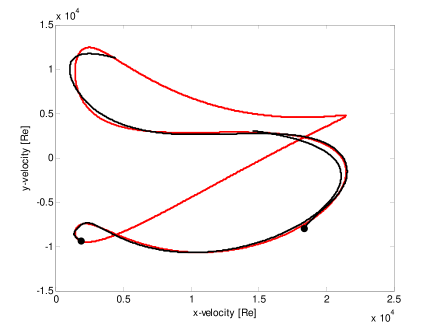
Figure 3: Example of Laguerre approximation for two components of a velocity history (arbitrary scaling). The red dot marks the present time. The red curve is the original cyclic signal and the black curves are Laguerre approximations for two different instants

4.5 Differential equation for Laguerre coefficients

In the finite element analysis, we need to update the Laguerre coefficients at each iteration of each time step, for every Gauss point of every node of the system. The explicit calculation of Equation 21 for every update is hence a CPU-time critical operation, taking in the order of $n\times N$ floating point operations (flops), where $n$ is the number of Laguerre polynomial used, and $N$ the number of time steps that the dual functions take to decay to a negligible value. Further, for each Gauss point, $2N$ velocity values need to be stored, a severe memory requirement.

In the present Section and the next it is shown how the computation of Equation 21 can be carried out by a recursive operation requiring no other storage than that of the Laguerre coefficients and the last velocity values, and taking in the order of $n\times n$ flops, which is advantageous because $n\ll N$. In this Section it is shown that $\overline{\tau}$ verifies a differential equation driven by the history $\overline{v}$ of the velocity component. In Section 4.6, this differential equation is solved time-step by time-step in a recursive update.

Equation 21 can be rewritten without matrix notation, and differentiated

$$\frac{\partial\tau_{i}}{\partial t} = \phantom{-\frac{1}{t_{w}}}\int_{0}^{+\infty}e^{-\theta}\mathcal{L}_{i}\left(\theta\right)\frac{\partial v}{\partial t}\left(t-t_{w}\theta\right)d\theta$$ (34)

$$= -\frac{1}{t_{w}}\int_{0}^{+\infty}e^{-\theta}\mathcal{L}_{i}\left(\theta\right)\frac{\partial v}{\partial\theta}\left(t-t_{w}\theta\right)d\theta$$ (35)

Multiplying by $t_{w}$ and integrating by parts yields

$$t_{w}\frac{\partial\tau_{i}}{\partial t}=-\left[e^{-\theta}\mathcal{L}_{i}\left(\theta\right)v\left(t-t_{w}\theta\right)\right]\\ +\int_{0}^{+\infty}\left[-e^{-\theta}\mathcal{L}_{i}\left(\theta\right)+e^{-\theta}\frac{\partial}{\partial\theta}\mathcal{L}_{i}\left(\theta\right)\right]\\ v\left(t-t_{w}\theta\right)d\theta$$ (36)

A property of Laguerre polynomials is

$$\frac{\partial}{\partial\theta}\mathcal{L}_{i}\left(\theta\right) = -\mathcal{L}_{i-1}^{{}^{(1)}}\left(\theta\right)$$ (37)

$$= -\sum_{j=0}^{{}^{i-1}}\mathcal{L}_{j}\left(\theta\right)$$ (38)

where $\mathcal{L}_{i}^{{}^{(1)}}\left(\theta\right)$ is a generalized Laguerre polynomial. Hence we can write

$$t_{w}\frac{\partial\tau_{i}}{\partial t}=\mathcal{L}_{i}\left(0\right)v\left(t\right)-\tau_{i}\\ -\int_{0}^{+\infty}e^{-\theta}\sum_{j=1}^{{}^{i-1}}\mathcal{L}_{j}\left(\theta\right)v\left(t-t_{w}\theta\right)d\theta$$ (39)

$$= v\left(t\right)-\tau_{i}-\sum_{j=1}^{{}^{i-1}}\tau_{j}$$ (40)

$$= v\left(t\right)-\sum_{j=1}^{{}^{i}}\tau_{j}$$ (41)

which is of the form

$$\frac{\partial\overline{\tau}}{\partial t}\left(t\right)=\overline{\overline{\mu}}\cdot\overline{\tau}\left(t\right)+\overline{n}\;v\left(t\right)$$ (42)

with

$$\begin{cases}\mu_{ij}=-\frac{1}{t_{w}}&\quad j\leq i\\ \phantom{\mu_{ij}}=0&\quad j>i\end{cases}$$ (43)

$$n_{i}=\frac{1}{t_{w}}$$ (44)

Equation 42 shows that at any time $t$, the rate of the Laguerre coefficients is fully defined by the Laguerre coefficients and the velocity signal.

4.6 Recursive filter

The discrete integration of Equation 42 must be done carefully, for two reasons. First it is important to obtain Laguerre coefficients that are independent of the sampling rate used (as long as the sampling rate is “adequate”). This is because the experimental data on which the VIV model is based may come from experiments which, after scaling, may have different sampling rates. Further, the numerical analysis in which the VIV model is used may use yet another time step. The choice of time step or sampling rate must not affect the way a trajectory is characterized by Laguerre coefficient.

The second reason for care in discrete integration is that we wish to be able to create synthesized signals $\overline{\overline{L}}\cdot\overline{\tau}$ of good quality. Synthesized signal are neither used in the numerical process of creating a force interpolation function (Section 5) or in the FEM use of the VIV model. However visualization is essential to the process of research, both for fault diagnosis and quality control, and to communicate an understanding of the method.

This discrete integration is only used in the analysis of experimental data, to provide an input to the training of the “rotatron” (Section 5.5). In dynamic analysis, the integration of Equation 42 is done by means of the Newmark-$\beta$ method, as detailed in Section 7.

Assume that velocity is sampled at regular intervals

$$v_{j}=v\left(t_{0}+j\,dt\right)$$ (45)

We seek the values of the Laguerre coefficients at the same intervals

$$\overline{\tau}_{j}=\overline{\tau}\left(t_{0}+j\,dt\right)$$ (46)

The vector $\overline{\tau}_{j}$ (the list of the coefficients for all Laguerre polynomial, take at step $j$) must not be confused with scalar $\tau_{i}$ (the coefficient for the Laguerre polynomial of degree $i$). We choose $t_{0}$ such that $t_{0}+j\,dt=0$, and we approximate $v$ by a function that is linear over the interval $[0,dt]$. Equation 42 becomes

$$\frac{\partial\overline{\tau}}{\partial t}\left(t\right)=\overline{\overline{\mu}}\cdot\overline{\tau}\left(t\right)+\overline{\alpha}+\overline{\beta}t$$ (47)

with

$$\overline{\alpha} = \overline{n}\,v\left(0\right)$$ (48)

$$\overline{\beta} = \overline{n}\,\frac{v\left(dt\right)-v\left(0\right)}{dt}$$ (49)

This new differential equation can be solved exactly: We seek a solution of the form

$$\overline{\tau}\left(t\right)=\exp\left(\overline{\overline{\mu}}\,t\right)\cdot\overline{a}+\overline{b}t+\overline{c}$$ (50)

over the interval. Here $\exp\left(\overline{\overline{\mu}}\,t\right)$ stands for a matrix exponential. Replacing this expression into Equation 47, noting that

$$\frac{\partial}{\partial t}\exp\left(\overline{\overline{\mu}}\,t\right) = \overline{\overline{\mu}}\cdot\exp\left(\overline{\overline{\mu}}\,t\right)$$ (51)

$$\exp\left(\overline{\overline{0}}\right) = \overline{\overline{I}}$$ (52)

and identifying the constant and linear terms and enforcing the initial value leads to

$$\overline{b} = -\overline{\overline{\mu}}^{-1}\cdot\overline{\beta}$$ (53)

$$\overline{c} = -\overline{\overline{\mu}}^{-2}\cdot\overline{\beta}-\overline{\overline{\mu}}^{-1}\cdot\overline{\alpha}$$ (54)

$$\overline{a} = \overline{\tau}\left(0\right)+\overline{\overline{\mu}}^{-2}\cdot\overline{\beta}+\overline{\overline{\mu}}^{-1}\cdot\overline{\alpha}$$ (55)

Replacing these expressions in Equation 50 at $t=dt$, a tedious but straightforward computation yields the recursive filter

$$\overline{\tau}_{j+1}=\overline{\overline{M}}\cdot\overline{\tau}_{j}+\overline{V}_{1}\cdot v_{j}+\overline{V}_{2}\cdot v_{j+1}$$ (56)

with

$$\overline{\overline{M}} = \exp\left(\overline{\overline{m}}\,dt\right)$$ (57)

$$\overline{\mu}_{1} = \overline{\overline{\mu}}^{-1}\cdot\overline{n}$$ (58)

$$\overline{\mu}_{2} = \overline{\overline{\mu}}^{-2}\cdot\overline{n}\,\frac{1}{dt}$$ (59)

$$\overline{V}_{1} = \overline{\overline{M}}\cdot\left(\overline{\mu}_{1}-\overline{\mu}_{2}\right)+\overline{\mu}_{2}$$ (60)

$$\overline{V}_{2} = \overline{\overline{M}}\cdot\overline{\mu}_{2}-\overline{\mu}_{1}-\overline{\mu}_{2}$$ (61)

5 Force interpolation

5.1 Foreword

This section details the implementation of point 4 in Section 2.4. This section presents an interpolation function which, given the Laguerre coefficients, predicts the present value of the force vector. Polynomials were considered initially, but is soon became clear that feed-forward “neural networks” provide a better class of functions to work with. The reason for that is that the number of polynomial coefficients of degree $d$ for a polynomial of $n$ variables is $n^{d}$, and high values of $d$ must be expected to be necessary. By contrast, in a neural network, non-linearity is introduced by “sigmoid” or “threshold” functions, and the coefficients are used to specify in which direction non-linearity applies. Further, polynomials are infamous for their propensity to oscillate.

The “rotatron” presented here is based on the “perceptron” [22, 21], a well studied architecture of neural network which provides a flexible tool for the interpolation of scalar-valued functions of a vector (Section 5.2). The rotatron takes advantage of certain symmetry properties of the physics at hand (Section 5.3).

In Section 7, the rotatron is used to predict scaled forces based on the Laguerre coefficients for scaled trajectories.

5.2 Perceptron

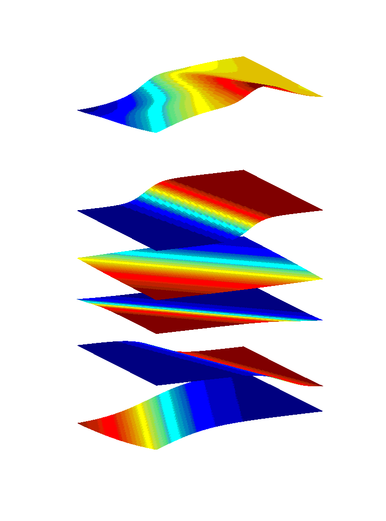
Figure 4: Perceptron: “arbitrary” functions (top) can be represented as a sum of sigmoid steps (bottom 5) of different orientation and steepness $N_{jkl}$, shift $V_{j}$, and height $M_{ij}$

A perceptron [22, 21] is a simple feed-forward neural network, consisting of 3 layers. The input layer has $2n$ neurons where $n$ is number of Laguerre coefficients for each velocity component and the factor 2 comes from the need to analyze in-line and cross-flow speed histories together. The values of the input layer neurons are set to the Laguerre coefficients for both velocity components. The second layer has $nhid$ neurons, whose values are an affine function of the values of the first layer, passed through a sigmoid function like

$$\sigma(x)=1-\frac{2}{e^{2x}+1}$$ (62)

Finally, the third layer gives the output of the perceptron, and its values are an affine function of the values of the second layer. This can be summarized as

$$\hat{f_{i}}=M_{ij}\cdot\sigma\left(N_{jkl}\cdot\tau_{kl}+V_{j}\right)+U_{i}$$ (63)

$M_{ij}$, $N_{jkl}$, $U_{i}$ and $V_{j}$ are the “weights” or interpolation coefficients, that must be adjusted to fit the perceptron to interpolate some given data. $\tau_{kl}$ are Laguerre coefficients and $\hat{f_{i}}$ are predicted force components. $i$ is the index of force direction ($x$ vs. $y$), $j$ the index of neuron in the hidden layer, $k$ the index of velocity direction and $l$ index of Laguerre coefficient.

Each output of the perceptron can be seen as a function, which is a sum of sigmoid steps (Figure 4).

5.3 Symmetries

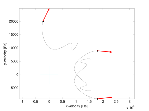
Figure 5: For circular cross section it is assumed that if two trajectories can deduced from each other by rotation or mirroring, then the corresponding forces are deduced from each other by the same operation

The relation between trajectories (in the sense of history of the velocity of the cylinder relative to the water) and forces can reasonably be assumed to exhibit several symmetries (Figure 5):

Rotational symmetry

If a trajectory can be deduced from the other by a rotation around the origin, then the resulting forces are also deduced from each other by the same rotation.

Mirror symmetry

If a trajectory can be deduced from the other by a mirroring around a line crossing the origin, then the resulting forces are also deduced from each other by the same mirroring.

Rotational symmetry and mirror symmetry together, imply directionality: If a trajectory is within a line crossing the origin, then the resulting forces are within the same line. In particular zero velocities must imply zero forces.

The symmetries imply that, once experimental data for a trajectory has been obtained, there is no need to acquire data for rotated or mirrored trajectories. However, if one was training a perceptron to interpolate the data, the training set would need to include trajectories and their rotates and mirrors, with the correspondingly rotated and mirrored forces. This would increase memory and CPU usage during training, but also during use of the trained perceptron, because the perceptron will need a larger number of hidden layer to interpolate the training data.

Another approach is hence used in the present work: the classic perceptron is replaced by a “rotatron” (Section 5.4). It is designed so that, whatever the values of the weight coefficient, a rotation or mirroring of the input trajectory results in the same rotation or mirroring of the output force vector.

5.4 Rotatron

A modified interpolation function (which will be refered to as “rotatron” in this text), which enforces the symmetries discussed in Section 5.3, is is defined as

$$\hat{f_{i}}=V_{k}\sigma_{ik}$$ (64)

with

$$\sigma_{ik} = \sigma_{i}\left(y_{[j]k}\right)$$ (65)

$$= \frac{y_{ik}}{|y_{[j]k}|\left(1+|y_{[j]k}|{}^{\alpha_{k}}\right)}$$ (66)

$$|y_{[j]k}| = \sqrt{y_{1k}^{2}+y_{2k}^{2}}$$ (67)

$$\alpha_{k} = -1-e^{-U_{k}}$$ (68)

$$y_{jk} = M_{kl}\,\tau_{jl}$$ (69)

In the above, index $i$ and $j$ refer to direction, index $l$ to the Laguerre polynomial and $k$ to the hidden layer. $V_{k}$, $U_{k}$ and $M_{kl}$ are tunable parameters. $\tau_{jl}$ are Laguerre coefficients, given as input to the “rotatron”. See Appendix A for conventions on index notations and in particular for the syntax $|y_{[j]k}|$. Note that Equations 21, 64 and 69 operate linearly, identicaly and independently on the terms related to the $x$ and $y$ directions, while Equation 66 involves a unit vector multiplied by a non linear function of its norm. Figure 6 illustrates the flow of information, from right to left, from two vectors containing the histories of the velocity components, to Laguerre coefficient, that are then processed in the rotatron.

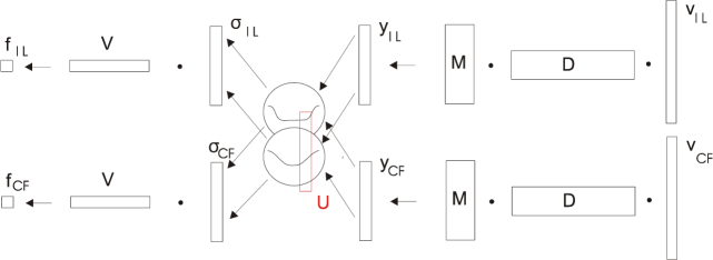
Figure 6: Laguerre analysis and rotatron transform velocity histories into a hydrodynamic force. The matrix $D$ is the discrete form of the Laguerre “duals”, which appear in Equation 21.

The non-linear function appearing in Equation 66 is a sigmoid, whose abruptness is parametrized by $U_{k}$ (Figure 7). The sigmoid is shown in Figure 7 for various values of the parameter $U_{k}$.

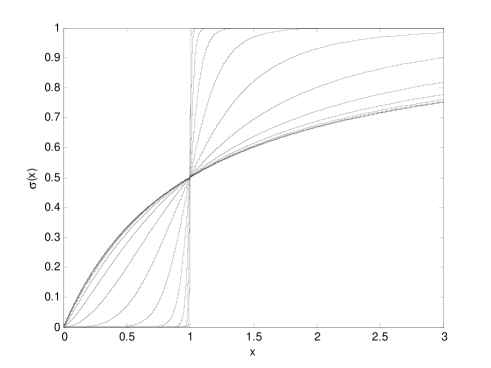
Figure 7: Log-logistic sigmoid functions

5.5 Training

“Training” of a neural network refers to finding weight coefficients $V_{k}$, $M_{kl}$ and, $U_{k}$ such that for any training point number $m$, consisting of Laguerre coefficients $\tau_{jlm}$ and two force components $f_{im}$, the outputs $\hat{f}_{im}$ computed by the neural network are close to $f_{im}$.

5.5.1 Regularization

A common problem when training neural networks is “overspecialization” [23]. In this situation, the neural network predicts the training outputs with high accuracy but behaves wildly between the training points. In contrast, what is implicitly sought is a smooth response of the network to the input, even if this means an imperfect fit to the training data.

Many strategies are described in the literature to address this problem. One of them, which is adopted here, is regularization [23]: the value of the weight parameters $V_{k}$, $M_{kl}$ and, $U_{k}$ are chosen by minimizing the cost function

$$J\left(V_{[k]},U_{[k]},M_{[k]},f_{[im]},\tau_{[jlm]}\right)=\\ \frac{1}{2}\left(f_{im}-\hat{f}_{i}\left(\tau_{[jl]m}\right)\right)^{2}+\rho\frac{1}{2}\left(U_{k}^{2}+V_{k}^{2}+M_{kl}^{2}\right)$$ (70)

where $\rho$ is the regularization coefficient, an arbitrary input to the training algorithm. High values of $\rho$ favor smoothness of the response of the neural network against precision in reproducing the training set.

5.5.2 Conjugate gradient optimization

$J$ is a function of a large number of weight coefficients, and hence it is not practical to compute the Hessian of $J$, because the Hessian is a full matrix. It also proves to be very costly to even compute an approximation to it as done in the Levenberg-Marquardt algorithm [7, 14]. On the other hand, the Nelder-Mead “downhill simplex” algorithm [19], which uses only the values of $J$, proved very slow in this case. Hence a search method is chosen, that determines the search direction from the gradient of $J$ [16]. This is a conjugate gradient method, in which the step length is found by deriving the gradient in the direction of the search. In this method, the positive definiteness of the (implicit) Hessian is forced by adding a scaled identity matrix to it, a technique known as “trust region”.

The conjugate gradient method proved far more efficient than the Levenberg-Marquardt and Nelder-Mead methods for the present task.

6 Metric

6.1 Euclidean metric and distance

In order to describe the available data, it is useful to define a distance between trajectories. This will allow to determine to what extend the set of available data “fills” the set of all possible trajectories, or to detect zones of transition from one hydrodynamic behavior to the other. Finally, this will help detecting contradictions in the available data, arising from a variety of sources, including hidden experimental variables, measurement uncertainties or inadequate modeling in inverse methods and not least, the natural variability of VIV forces.

The $x$ and $y$ components of a trajectory are described by a pair of functions:

$$\overline{f}\equiv\left(\overline{f}_{x},\overline{f}_{y}\right)$$ (71)

We can define a scalar product between trajectories, that captures any recent differences:

$$\overline{f}^{T}\diamond\overline{g}\equiv\overline{f}_{x}^{T}\circ\overline{\overline{W}}\circ\overline{g}_{x}+\overline{f}_{y}^{T}\circ\overline{\overline{W}}\circ\overline{g}_{y}$$ (72)

$$=\intop_{-\infty}^{0}\frac{e^{\frac{t}{t_{w}}}}{t_{w}}\left(f_{x}(t)g_{x}(t)+f_{y}(t)g_{y}(t)\right)dt$$ (73)

By replacing $\overline{f}_{x}$, $\overline{f}_{y}$, $\overline{g}_{x}$ and $\overline{g}_{y}$ by their expression in terms of Laguerre polynomials and their respective Laguerre coefficients $\overline{\tau}_{fx}$, $\overline{\tau}_{fy}$, $\overline{\tau}_{gx}$ and $\overline{\tau}_{gy}$, one finds that

$$\overline{f}^{T}\diamond\overline{g} = \overline{\tau}_{fx}^{T}\cdot\overline{\tau}_{gx}+\overline{\tau}_{fy}^{T}\cdot\overline{\tau}_{gy}$$ (74)

$$= \overline{\tau}_{f}^{T}\cdot\overline{\tau}_{g}$$ (75)

with

$$\overline{\tau}_{f}\equiv\left[\begin{array}[]{c}\overline{\tau}_{fx}\\ \overline{\tau}_{fy}\end{array}\right],\quad\overline{\tau}_{g}\equiv\left[\begin{array}[]{c}\overline{\tau}_{gx}\\ \overline{\tau}_{gy}\end{array}\right]$$ (76)

The distance is defined from the scalar product in the usual manner:

$$\left|\overline{f}-\overline{g}\right| \equiv \sqrt{\left(\overline{f}-\overline{g}\right)^{T}\diamond\left(\overline{f}-\overline{g}\right)}$$ (77)

$$= \left|\overline{\tau}_{f}-\overline{\tau}_{g}\right|$$ (78)

In other words, neighboring vectors of Laguerre coefficients describe trajectories that are similar in the recent past. This is illustrated by taking random samples of Laguerre coefficients around a given value obtained from data analysis and plotting the synthesized trajectories (Figure 8).

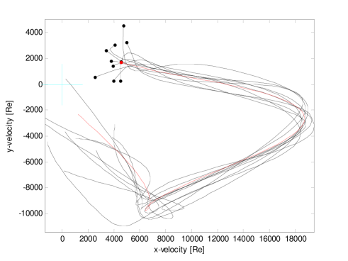
Figure 8: A set of neighboring trajectories according to Equation 78. Typical distance between trajectories: $10^{3}\;[ilr\,Re]$.

6.2 Rotatron-distance

The above does not account for rotational and mirror symmetries. We seek a distance for which the distance of a trajectory to its transforms by rotation or mirroring is zero. Another distance is hence introduced:

$$d\left(\overline{f},\overline{g}\right)\equiv\\ \min\left(\min_{R\in\mathfrak{R}}\left|\overline{f}-R\left(\overline{g}\right)\right|\;,\;\min_{S\in\mathfrak{S}}\left|\overline{f}-S\left(\overline{g}\right)\right|\right)$$ (79)

where $\mathfrak{R}$ is the set of all rotations of the trajectories around the origin and $\mathfrak{S}$ the set of all mirroring of trajectories around a line passing by the origin. Note that no norm or scalar product associated to the distance $d$ is presented here (The vector-space of trajectories, divided by the group of rotations and mirrorings, is not a vector space).

Because $\overline{f}_{x}$ is related to $\overline{\tau}_{fx}$ by the same linear relation that relates $\overline{f}_{y}$ to $\overline{\tau}_{fy}$, linear combinations of $\overline{f}_{x}$ and $\overline{f}_{y}$ (including rotation and mirroring) are related to the same linear combinations on $\overline{\tau}_{fx}$ and $\overline{\tau}_{fy}$. By expressing the distance $\left|\overline{f}-R\left(\overline{g}\right)\right|$ as a function of the angle $\alpha$ of the rotation $R$, and then differentiating with respect to $\alpha$, it can be shown that the value of $\alpha$ that minimizes $\left|\overline{f}-R\left(\overline{g}\right)\right|$ is

$$\alpha=\arctan\\ \left(\overline{\tau}_{fx}\cdot\overline{\tau}_{gy}-\overline{\tau}_{fy}\cdot\overline{\tau}_{gx}\;,\;\overline{\tau}_{fy}\cdot\overline{\tau}_{gy}+\overline{\tau}_{fx}\cdot\overline{\tau}_{gx}\right)$$ (80)

where $\arctan\left(y,x\right)\in\left]-\pi,\pi\right]$ is the angle of a vector $\left[x,y\right]^{T}$ with the $x$-axis. Similarly, it can be shown that the mirroring that minimizes $\left|\overline{f}-S\left(\overline{g}\right)\right|$ is the composition of a rotation of angle

$$\beta=\arctan\\ \left(\overline{\tau}_{fx}\cdot\overline{\tau}_{gy}+\overline{\tau}_{fy}\cdot\overline{\tau}_{gx}\;,\;\overline{\tau}_{fy}\cdot\overline{\tau}_{gy}-\overline{\tau}_{fx}\cdot\overline{\tau}_{gx}\right)$$ (81)

by a swap of the sign of the $x$-coordinates. Equations 80 and 81 allow to compute 79.

Figure 9 shows a trajectory and the trajectories within a small database that have the smallest distance to it, measured using $d$.

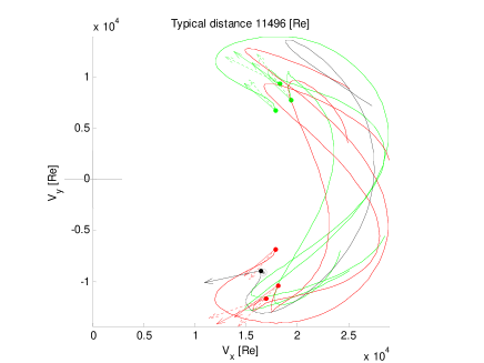
Figure 9: A trajectory and its neighbors in terms of rotatron distance. Smooth curve: Laguerre approximation of trajectory, stippled arrow: true force, smooth arrow: predicted force. Black is for the trajectory used to enter the model to find the force. Green and red are used for the three closest points in the database, respectively before and after rotation or mirroring.

6.3 Fractal dimension

Considering a relatively uniform cloud of points, the number $m$ of points in a sphere is proportional to the radius $r$ of the sphere to the power of $p$, where $p$ is the dimension of the space in which the cloud is defined. For example, using $2\times 10$ coefficients to describe both components of a trajectory, if the database was filling this space, the number of points within the sphere would be $m\propto r^{20}$ (no realistic experimental database can “fill” such a volume).

Conversely, one can define the fractal dimension (or Minkowski-Bouligand dimension [13]) $p$ of a set (in particular, of a “database” of Laguerre coefficients) by counting the number $m(r)$ of pairs of points in the set which have a distance smaller than $r$:

$$p(r)\equiv\frac{\partial\log m(r)}{\partial\log r}$$ (82)

One should either smooth $m(r)$ or compute the derivative by finite differences over a large enough interval. Note that the fractal dimension $p$ is a function of the scale $r$.

Imagine that we have a series of data-points $(x,y,z)$, and we are investigating whether $z$ can be predicted using $x$ and $y$. Let us imagine that the fractal dimension of the set of $(x,y)$ pairs is $2$ (the set of $(x,y)$ fills the plane). If the fractal dimension of the set of $(x,y,z)$ is equal to $2$, then the set of $(x,y,z)$ is within a surface, and $z$ can be predicted using $x$ and $y$. If the fractal dimension of the set of $(x,y,z)$ is equal to $3$, the data forms a cloud, and $x$ and $y$ are not sufficient to predict $z$, other hidden variables must be at play. These concepts are now applied to the study of the database.

Figure 10 shows the cumulative distribution of the distances between trajectories (black curve) computed using Equation 79. $p$ is seen to depend on the scale on the scale: from afar ($r>2\times 10^{4}\;[ilr\,Re]$), the slope of the curve is zero, hence the dimension is zero: all the data are lumped into a point. Zooming into the data set ($r=3\times 10^{3}\;[ilr\,Re]$) one can discern a cloud of dimension $4.76$. At $r=1.5\times 10^{3}\;[ilr\,Re]$ the slope decreases to about $p=2$, and it is believed that this is the dimension of the dataset for a given point along the riser. At small scale ($r<1\times 10^{3}\;[ilr\,Re]$), the dimension increases again, possibly due to noise in the data. or weaknesses in the Laguerre approximation.

The red curves in Figure 10 are computed by adding the sum of squares of the differences between force components (suitably scaled) to the squares of the distances between trajectories, and then extracting the square root. The four red curves are drawn using the original force data, to which Gaussian noise of standard deviation $0,$ $10^{7}$, $10^{8}$ and $10^{9}\>[N/m]$ respectively has been added. The standard deviation of the original force is about $2\times 10^{8}\>[N/m]$ . The two first red curves are indistinguishable, which seems to indicate that we cannot expect to achieve a 10% precision in force predictions. The marked difference with curves 3 and 4 shows however that we have assets in hand to predict the force. Similar curves have been produced with added noise of standard deviations $1\times 10^{7}$, $2\times 10^{7}$… $10\times 10^{7}\;[N/m]$, and already at $2\times 10^{7}\;[N/m]$ the curve is distinct from the one based on the original data.

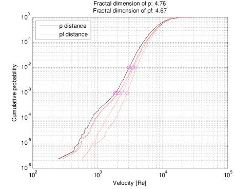
Figure 10: Computing fractal dimensions

7 Dynamic analysis

7.1 Foreword

Once it is possible to predict hydrodynamic forces on a cross section for a given velocity history, the next development is to include the force thus predicted in a dynamic time domain simulation. Because the VIV forces introduce severe non-linearities, a naive connection (where the forces are just added to the right hand side of the system) might lead to slow convergence, or to divergence of the Newton-Raphson iterations used at each time step. To obtain a proper formulation, it is necessary to jointly treat the system of differential equations composed of the state equations of the structure, and the differential equations (42) followed by the Laguerre coefficient. However in doing so, for each displacement degree of freedom, $n$ Laguerre coefficients are added, and it is crucial for efficiency to eliminate them before solving a large linear system of equations.

To this effect, in this Section, the following sequence of transformations is applied to the differential equations:

1. The differential equations are first set in incremental form (Section 7.3).

2. Time discretization by the Newmark-$\beta$ method is introduced (Section 7.4).

3. The Laguerre coefficients are condensed out of the system of equations (Section 7.5).

4. Finite element interpolation is introduced (space discretisation), using Gauss quadrature (Section 7.6).

This particular sequence leads to a VIV model that is implemented at the Gauss point level, and can easily be introduced in a general purpose FEM software with standard, displacement based beam or cable elements. Another sequence, 1, 4, 2, 3, can be used to obtain either a hybrid element, or alternatively, a mixed element which would require a specialized solver for optimal efficiency. These alternatives are more difficult to integrate into existing software working with displacement based elements, and are not discussed here.

7.2 Differential equations

The dynamic differential equation of a 3D beam subjected to VIV loads can be formalized as

$$r_{di}\left(x_{[bj]},\dot{x}_{[bj]},\ddot{x}_{[bj]},t\right)\\ =\lambda_{Nm^{-1}}^{-1}\hat{f}_{d}\left(\tau_{[pb]i}\right)+E_{di}$$ (83)

where Newton’s “dot” notation for a time derivative stands for a derivation with respect to unscaled time $t$, as opposed to scaled time $t^{*}$, and with [17, 5]

$$E_{di} = C_{L}\,\rho\nu\left(\dot{w}_{di}-\dot{x}_{di}\right)$$ (84)

$$+ C_{Q}\,\frac{1}{2}\rho D_{i}\left|\dot{w}_{di}-\dot{x}_{di}\right|\left(\dot{w}_{di}-\dot{x}_{di}\right)$$

$$+ C_{M}\frac{\pi}{4}\rho D_{i}^{2}\left(\ddot{w}_{di}-\ddot{x}_{di}\right)$$

$$+ \hphantom{C_{M}}\frac{\pi}{4}\rho D_{i}^{2}\ddot{w}_{di}$$

The four terms in the above Morison’s equation are the linear drag, the quadratic drag, the sum of diffraction and added mass forces, and the Froude-Krylov forces. The fourth term introduces the correction discussed in Section 3.1.

If $C_{L}$, $C_{Q}$ or $C_{M}$ are set to values different from zero, then it is necessary to substract the correspond values from the forces $f_{di}$ used to train the rotatron. Experience shows that the Using $C_{M}=1$, $C_{Q}=1$ and $C_{L}=0$ contributes to the stability of the dynamic analysis.

Equation 42 must be scaled to keep only derivatives with respect to unscaled time, for the application of Newmark-$\beta$ (Section 7.4)

$$\frac{\partial\tau_{lbi}}{\partial t^{*}}=\mu_{lp}\tau_{pbi}+n_{l}\lambda_{ms}^{-1}\left(\dot{x}_{bi}-\dot{w}_{bi}\right)$$ (85)

so that

$$\lambda_{s}^{-1}\dot{\tau}_{lbi}=\mu_{lp}\tau_{pbi}+n_{l}\lambda_{ms^{-1}}\left(\dot{x}_{bi}-\dot{w}_{bi}\right)$$ (86)

The indices $d$ and $b$ span pairs of directions, orthogonal to the cylinder. Indices $i$ and $j$ stand for positions along the cylinder, and span a continuous set of values (coordinates along the cylinder). Indices $l$ and $p$ refer to the Laguerre coefficients of various degrees. Forces $\hat{f}_{di}=\hat{f}_{d}\left(\tau_{[pb]i}\right)$ at location $i$ only depend on the Laguerre coefficients $\tau_{pbi}$ for the same location. At that location, the force component in direction $d$ depend on the Laguerre coefficients of all degrees $b$ for both directions $p$. $\rho$ is the fluid density $\ddot{w}_{di}$ is the acceleration of the undisturbed fluid. $\frac{\pi}{4}\rho D_{i}^{2}\ddot{w}_{di}$ stands for the Froude-Krylov forces. Diffraction forces are present in the laboratory tests and hence accounted for by $\hat{f}_{d}$.

7.3 Incremental form

The incremental form of Equations 83 and 86is

$$r_{di}+k_{dibj}dx_{bj}+c_{dibj}d\dot{x}_{bj}+m_{dibj}d\ddot{x}_{bj}\\ =\lambda_{Nm^{-1}}^{-1}\hat{f}_{di}+h_{dipbj}d\tau_{pbj}+E_{di}$$ (87)

$$\lambda_{s}^{-1}\left(\dot{\tau}_{lbi}+d\dot{\tau}{}_{lbi}\right)=\mu_{lp}\left(\tau_{pbi}+d\tau_{pbi}\right)\\ +n_{l}\lambda_{ms^{-1}}\left(\dot{x}_{bi}+d\dot{x}{}_{bi}-\dot{w}_{di}\right)$$ (88)

with

$$k_{dibj} = \dfrac{\partial r_{di}}{\partial x_{bj}}$$ (89)

$$c_{dibj} = \dfrac{\partial r_{di}}{\partial\dot{x}_{bj}}+C_{Q}\rho D_{i}\delta_{ij}\left[\vphantom{\frac{A}{A}}\left|\dot{w}_{[p]i}-\dot{x}_{[p]i}\right|\delta_{bd}\right.$$ (90)

$$+\left.\vphantom{\frac{A}{A}}\left(\dot{w}_{di}-\dot{x}_{di}\right)\left(\dot{w}_{bi}-\dot{x}_{bi}\right)\left|\dot{w}_{[p]i}-\dot{x}_{[p]i}\right|^{-1}\right]$$

$$+C_{L}\rho\nu\delta_{ij}\delta_{bd}$$

$$m_{dibj} = \dfrac{\partial r_{di}}{\partial\ddot{x}_{bj}}+C_{M}\frac{\pi}{4}\rho D_{i}\delta_{ij}\delta_{bd}$$ (91)

$$h_{dipbj} = \lambda_{Nm^{-1}}^{-1}\dfrac{\partial\hat{f}_{di}}{\partial\tau_{pb}}\delta_{ij}$$ (92)

The expression for $\frac{\partial\hat{f}_{di}}{\partial\tau_{pb}}$ is presented in Appendix B.

7.4 Time discretization

Newmark-$\beta$ is a method geared towards 2nd order differential equations. Equation 88, however, is only of the first order, and this opens two options: we can treat Equation 88 as being of the second order in $\tau_{lbi}$, but with the coefficient of $\ddot{\tau}_{lbi}$ being zero. Alternatively, we can introduce the antiderivative $T_{lbi}$ of $\tau_{lbi}$, and treat Equation 88 as being of the second order in $T_{lbi}$, but with the coefficient of $T_{lbi}$ being zero. The later option was chosen, based on the weak justification that this treats $\tau_{lbi}$ and $\dot{x}_{bj}$ both as first derivatives, which seems natural considering Equation 21.

Applying Newmark-$\beta$ to Equations 87 and 88 in this way yields

$$\forall d,i,\;\left[k_{dibj}+\frac{\gamma}{\beta dt}c_{dibj}+\frac{1}{\beta dt^{2}}m_{dibj}\right]dx_{bj}\\ -\frac{\gamma}{\beta dt}h_{dipbj}dT_{pbj}\\ =\lambda_{Nm^{-1}}^{-1}\hat{f}_{di}+E_{di}-r_{di}\\ +c_{dibj}b_{bj}^{x}+m_{dibj}a_{bj}^{x}-h_{dipbj}b_{pbj}^{\tau}$$ (93)

and

$$-\frac{\gamma}{\beta dt}n_{l}\lambda_{ms^{-1}}dx_{bi}+\left[\frac{1}{\beta dt^{2}}\lambda_{s}^{-1}\delta_{lp}-\frac{\gamma}{\beta dt}\mu_{lp}\right]dT_{pbi}\\ =n_{l}\lambda_{ms^{-1}}\left(\dot{x}_{bi}-\dot{w}_{bi}\right)+\mu_{lp}\tau_{pbi}-\lambda_{s}^{-1}\dot{\tau}_{lbi}\\ -n_{l}\lambda_{ms^{-1}}b_{bi}^{x}-\mu_{lp}b_{pbi}^{\tau}+a_{lbi}^{\tau}$$ (94)

with

$$a_{bj}^{x} = \frac{1}{\beta dt}\dot{x}_{bj}+\frac{1}{2\beta}\ddot{x}_{bj}$$ (95)

$$b_{bj}^{x} = \frac{\gamma}{\beta}\dot{x}_{bj}+\left(\frac{\gamma}{2\beta}-1\right)dt\,\ddot{x}_{bj}$$ (96)

$$a_{pbj}^{\tau} = \frac{1}{\beta dt}\tau_{pbj}+\frac{1}{2\beta}\dot{\tau}_{pbj}$$ (97)

$$b_{pbj}^{\tau} = \frac{\gamma}{\beta}\tau_{pbj}+\left(\frac{\gamma}{2\beta}-1\right)dt\,\dot{\tau}_{pbj}$$ (98)

For refinement iterations, $a_{bj}^{x}$, $b_{bj}^{x}$, $a_{pbj}^{\tau}$ and $b_{pbj}^{\tau}$ are set to zero. Typicaly, $\gamma=$$\frac{1}{2}$, $\beta=\frac{1}{4}$. The step $dt$ refers to unscaled time.

As usual in the Newmark-$\beta$ method, the increments for the time derivatives are found from the increment as

$$d\dot{x}_{bj} = \frac{\gamma}{\beta dt}dx_{bj}-b_{bj}^{x}$$ (99)

$$d\ddot{x}_{bj} = \frac{1}{\beta dt^{2}}dx_{bj}-a_{bj}^{x}$$ (100)

$$d\tau_{pbj} = \frac{\gamma}{\beta dt}dT_{pbj}-b_{pbj}^{\tau}$$ (101)

$$d\dot{\tau}_{pbj} = \frac{1}{\beta dt^{2}}dT_{pbj}-a_{pbj}^{\tau}$$ (102)

7.5 Condensation

The time discrete equations can be rewritten in a compact form:

$$s_{dibj}^{1}dx_{bj}-s_{dipbj}^{2}dT_{pbj} = s_{di}^{3}$$ (103)

$$s_{l}^{4}dx_{bi}+s_{lp}^{5}dT_{pbi} = s_{lbi}^{6}$$ (104)

with

$$s_{dibj}^{1} = k_{dibj}+\frac{\gamma}{\beta dt}c_{dibj}+\frac{1}{\beta dt^{2}}m_{dibj}$$ (105)

$$s_{dipbj}^{2} = \frac{\gamma}{\beta dt}h_{dipbj}$$ (106)

$$s_{di}^{3} = \lambda_{Nm^{-1}}^{-1}\hat{f}_{di}+E_{di}-r_{di}$$ (107)

$$+c_{dibj}b_{bj}^{x}+m_{dibj}a_{bj}^{x}$$

$$-h_{dipbj}b_{pbj}^{\tau}$$

$$s_{l}^{4} = -\frac{\gamma}{\beta dt}n_{l}\lambda_{ms^{-1}}$$ (108)

$$s_{lp}^{5} = \frac{1}{\beta dt^{2}}\lambda_{s}^{-1}\delta_{lp}-\frac{\gamma}{\beta dt}\mu_{lp}$$ (109)

$$s_{lbi}^{6} = n_{l}\lambda_{ms^{-1}}\left(\dot{x}_{bi}-\dot{w}_{bi}\right)+\mu_{lp}\tau_{pbi}-\lambda_{s}^{-1}\dot{\tau}_{lbi}$$ (110)

$$-n_{l}\lambda_{ms^{-1}}b_{bi}^{x}-\mu_{lp}b_{pbi}^{\tau}+\lambda_{s}^{-1}a_{lbi}^{\tau}$$

One can then condense $dT_{pbi}$ out of the above system of equations:

$$dT_{pbj}=\left(s^{5}\right)_{pl}^{-1}\left(s_{lbj}^{6}-s_{l}^{4}dx_{bj}\right)$$ (111)

$$\left[s_{dibj}^{1}+s_{dipbj}^{2}\left(s^{5}\right)_{pl}^{-1}s_{l}^{4}\right]dx_{bj}\\ =s_{di}^{3}+s_{dipbj}^{2}\left(s^{5}\right)_{pl}^{-1}s_{lbj}^{6}$$ (112)

Equation 112 is forced into “Newmark” form as

$$\left[k_{dibj}^{*}+k_{dibj}+\frac{\gamma}{\beta dt}c_{dibj}+\frac{1}{\beta dt^{2}}m_{dibj}\right]dx_{bj}\\ =\hat{f}_{di}^{*}-r_{di}+c_{dibj}b_{bj}^{x}+m_{dibj}a_{bj}^{x}$$ (113)

with

$$k_{dibj}^{*} =s_{dipbj}^{2}\left(s^{5}\right)_{pl}^{-1}s_{l}^{4}$$ (114)

$$\hat{f}_{di}^{*} =\lambda_{Nm^{-1}}^{-1}\hat{f}_{di}+E_{di}-h_{dipbj}b_{pbj}^{\tau}$$

$$+s_{dipbj}^{2}\left(s^{5}\right)_{pl}^{-1}s_{lbj}^{6}$$ (115)

$k_{dibj}^{*}$and $\hat{f}_{di}^{*}$ both depend on $dt$, $\beta$ and $\gamma$: The symbol $k_{dibj}^{*}$ was chosen to indicate that the matrix is handled by the Newmark-$\beta$ solver in the same way as a stiffness, however this terms can not be interpreted physically as a stiffness.

7.6 Spacial discretization

The consistent discretisation by Galerkin finite elements of Equation 113 leads to

$$K_{nm}^{*} = N_{din}k_{dibj}^{*}N_{bjm}$$ (116)

$$\hat{F}_{n}^{*} = N_{din}\hat{f}_{di}^{*}$$ (117)

$K_{nm}^{*}$ and $\hat{F}_{n}^{*}$ are typicaly computed by Gauss quadrature. Note that no space derivative is present in $k_{dibj}^{*}$, so no partial integration or Gauss quadrature with curvature shape function appears. One can hence simplify the expression of the element matrix to

$$K_{nm}^{*}=N_{din}k_{dib}^{*}N_{bim}$$ (118)

which means “same quadrature as for a mass matrix”.

7.7 Implementation

In non-linear FEM code, incremental matrices and vectors are computed by Gauss quadrature. The Gauss quadrature involves shape functions, tensors that are local, continuous versions of the stiffness, damping and mass matrices, and the force imbalance vector. For example for the drag damping of a beam element, the tensor relates a vector which components are increments in velocities in three directions, to another vector which components are increments in forces per unit length in three directions.

Within an iteration, the linear solver provides incremental nodal positions, velocities and accelerations for the model. These are disassembled and provided to the elements. The elements compute positions, velocities and accelerations (and more) in a co-rotated reference system at Gauss points. The resulting values are handed to the VIV-Gauss point procedure.

The axial velocities are discarded. The procedure scales the provided values using Equations 4 and 5.

Having stored the previous approximation of the scaled position, the procedure determines the position increment $dx_{bj}$, and then uses Equation 111 to obtain the Laguerre coefficient increment $dT_{pbj}$. From there, Equations 101 and 102 are used to compute $d\tau_{pbj}$ and $d\dot{\tau}_{pbj}$ . The values of $T_{pbj}$, $\tau_{pbj}$ and $\dot{\tau}_{pbj}$ are updated from previously stored values. $\tau_{pbj}$ is then used to evaluate $\hat{f}_{di}$ and its derivative with respect to $\tau_{pbj}$. These are scaled back, and Froude-Krylov forces are added, leading to $k_{dibj}^{*}$ and $\hat{f}_{di}^{*}$.

The above matrix and vector are padded with zeros to indicate zero force in the axial direction and zero torque.

The condensation of a larger system of time-discretized equations introduces some inelegant features compared to standard dynamic FEM: the VIV-Gauss point must be provided with $\beta$, $\gamma$ and $dt$ and a flag showing wether a call is made at a step or within a refinement iteration.

Note that the dynamic FEM computation does not make any use of the recursive filter presented in Section 4.6: this filter is used only in the training of the rotatron model. In the context of training, the filter had the advantage of making refinement iterations unnnecessary. It further allowed to avoid using Newmark-$\beta$ in a situation with prescribed displacement, for which it is not well suited.

8 Results

8.1 Training

The Norwegian Deepwater Program was a research effort in which reduced scale tests were carried out on long, flexible riser models, subject to uniform or sheared current [3]. The displacement histories thus aquired at 19 points along the riser model were later prescribed on short stiff cylinders, and the hydrodynamic forces acting on the cylinders directly measured [decao10]. The data from [decao10] that is used in this work consists of the displacements at 19 points along the NDP riser model, for 3 current profiles (Table 1), so a total of 57 short cylinder runs. For each of the 57 runs, 100 instants are randomly selected, yielding a training set of the rotatron with 5700 “points”. Each “point” consistes of two sets of $n=30$ Laguerre coefficients and the two components of the corresponding force (Figure 11).

Test name	Reynolds number	Current
TN2030	13500	uniform
TN2340	0-16200	shear
TN2370	0-24300	shear

Table 1: Reynolds number in NDP tests

The rotatron was trained using $n=30$ Laguerre polynomials, 200 neurons in the hidden layer, and 50 to 1000 iterations of the conjugate gradient optimization algorithm.

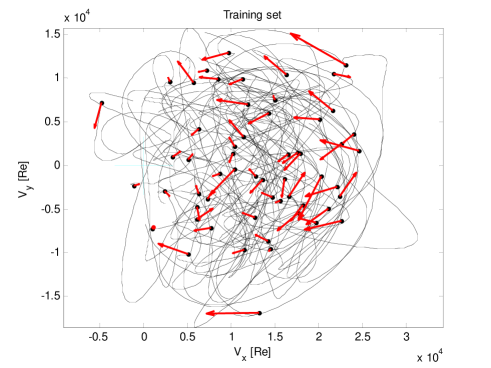
Figure 11: Force vector and Laguerre approximation of velocity, for a fraction (1%) of the data used to train the rotatron. The blue cross marks the origin (zero velocity relative to water)

Figure 12 shows how the rotatron predicts the forces for the trajectories in the above-mentionned 57 runs of short cylinder tests. the comparison of the forces aquired experimentaly with the forces predicted using the model. The model’s ability to predict these forces seems to be good, although we lack a good criteria to judge that yet.

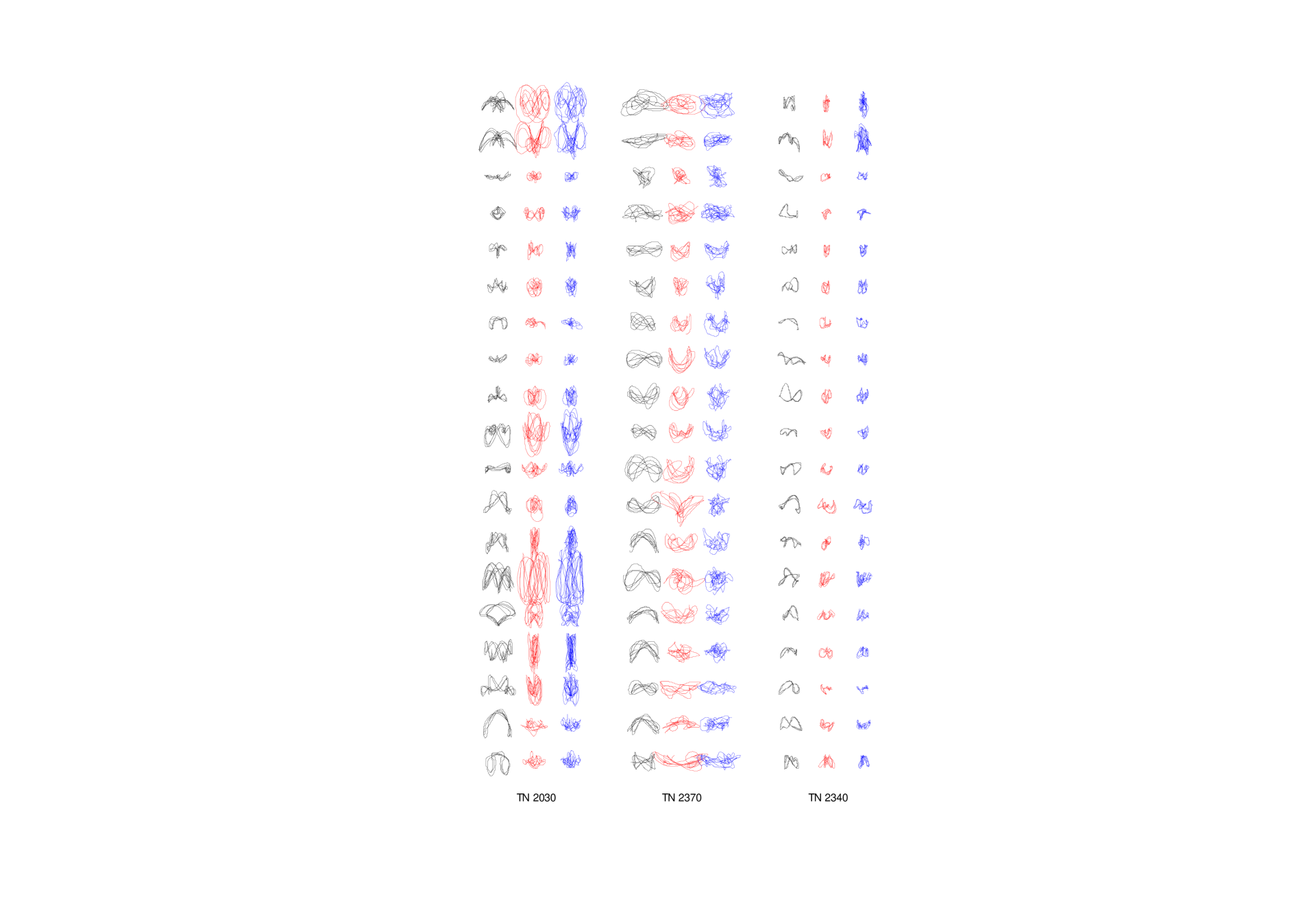
Figure 12: Quality of prediction on the training data set. Velocity (black), training force (red), predicted force (blue). All velocities and all forces presented at the same scales

Figure 13 provides a visualisation of the different steps of the modelisation process, and is hence a useful diagnostic tool. It shows:

Stippled_black_line

The trajectory for which a force prediction is wanted.

Smooth_black_line

The Laguerre approximation to the above trajectory, used to enter the rotatron.

Stippled_black_arrow

The measured force for the above trajectory.

Smooth_black_arrow

The predicted force for the above trajectory.

Green

Neighboring (in the sense of the rotatron distance, Equation 79) trajectories from experiments, used in the training set (and corresponding Laguerre approximation, experimentally measured force and predicted force).

Red

Same as the above after rotation and/or mirroring.

Figure 13 gives an indication of the quality of the Laguerre approximation, the adequacy of the training set for the trajectory at hand, the presence of contradictions in the training set near the trajectory at hand, the quality of the fit of the rotatron to the training data and finally the quality of the interpolation between training points.

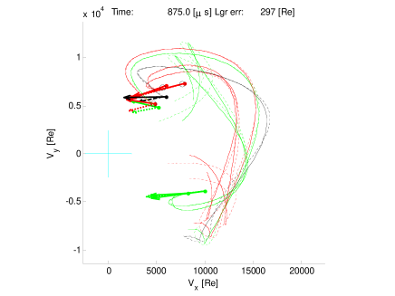
Figure 13: Illustration of the approximation process. See Section 8.1

8.2 Dynamic analysis of a flexible riser

VIV depends not only of current velocities, but on the type of slender system they act upon. Tension, stiffness, damping, length and boundary conditions affect the vibration and hence the velocity trajectories that appear in the vibration. Hence the database used in Section 8.1 to train the rotatron is specialised, not only to a few Reynolds numbers for the current velocity, but also to some extend to the particular model used in the NDP program. No study was carried out in this work on which changes in the structure change its way of vibrating to the point were the rotatron provides poor for estimations for it.

Hence, in order to test the performance of the present VIV model within a dynamic analysis, the simplest case was considered: the riser model used in the NDP testing program ([3], characteristics in Table 2) was modelled. The present method was used to analyse the test condition TN2370 ($0-24300\,Re$). Numerical results were compared with those obtained experimentaly on the NDP model. A laptop, using one core of a dual core processor, took 20 to 50 seconds to compute one second of riser response.

Quantity	Value
length	$38$	$m$
outer diameter	$0.027$	$m$
$EI$	$37.2$	$Nm^{2}$
$EA$	$5.09\cdot 10^{5}$	$N$
mass	$0.933$	$kg/m$
tension	$3000$	$N$

Table 2: Characteristics of the NDP reduced scale riser model

In Figures 14 and 15, the horizontal axis is NDP-laboratory time, the vertical axis is the unscaled length along the riser. The upper subplot shows the response in line (IL) with the flow, the lower subplot the cross-flow (CF) response. The color codes the displacements, with the same color scale used in Figures 14 to 16.

Figures 14 and 15 are for test TN2370 ($0-24300\>Re$). The dynamic simulations captures the frequency doubling between CF and inline, as well as the instationary nature of the vibrations. Frequency and amplitude are adequately captured. The 6th mode’s dominance of the CF vibration is correctly captured. The dynamic analysis assumes constant tension. By contrast, some small tension modulations seem to displace the position of the lower vibration node in the test. In test 2370 there is a marked tendency for CF vibrations to propagate downwards. In the analysis results, CF waves are of a more static character. The IL vibration in the analysis occurs at a higher mode (11) than in the test (9). This is best seen by counting red dots along diagonals, for example starting from coordinate $38m$ and time $17.9s$ in Figure 14. As a consequence, and since, for a given propagation celerity, wavelength and period are related, the phase drift between IL and CF are of opposite sign in the analysis and the test.

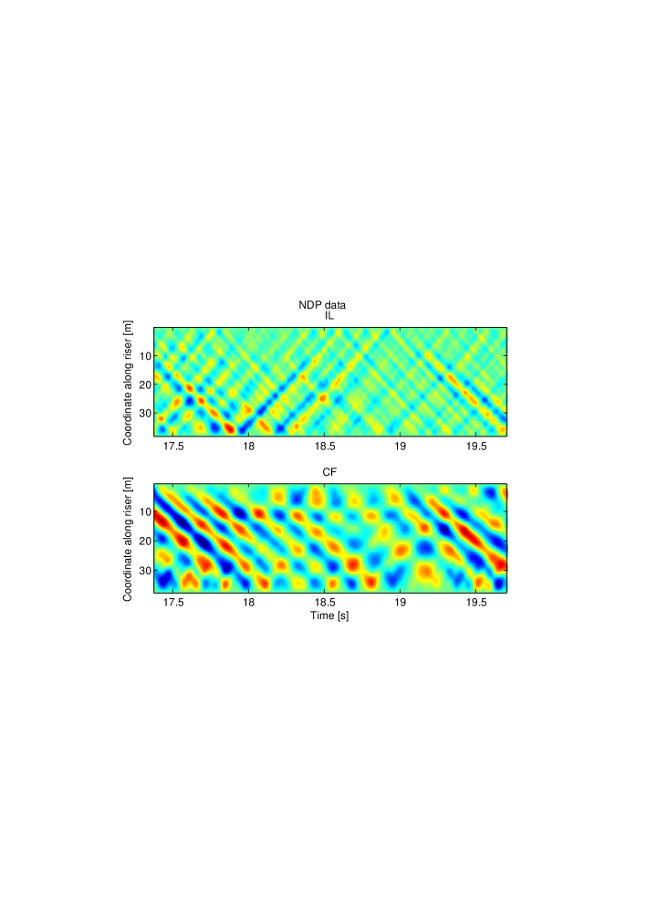
Figure 14: NDP test results, test 2370 ($0-24300\>Re$). The color coding describes the displacement

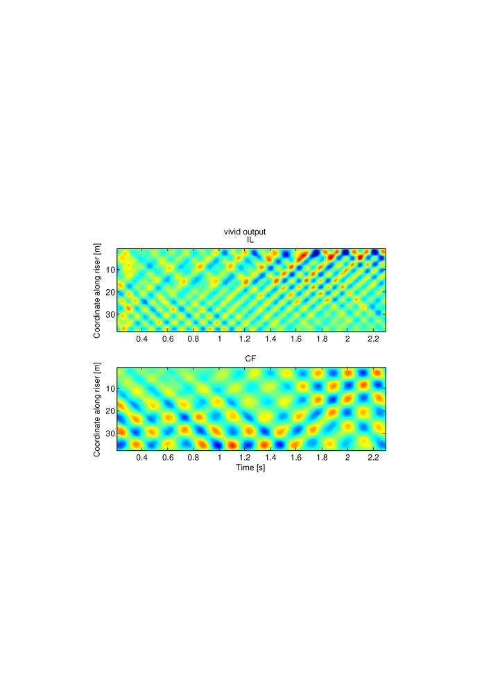
Figure 15: Analysis results, test 2370 ($0-24300\>Re$)

It proved impossible to reproduce tests 2340 and 2030 in the same manner. The analysis quickly ends with IL and CF vibrations occurring at the same frequency, and in Figure 16, with in-line motions dominating.

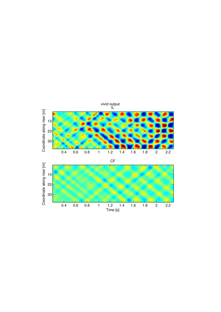
Figure 16: Analysis results, test 2030 ($13500\,Re$)

9 Discussion

9.1 Force prediction

Figure 12 shows that given the velocities in the training data as input, the model allows to reproduce the forces in the training data, based on the velocity in the training data.

The same exercise is carried out with trajectories from another test, N2430 (not to be confused with TN2340), which was carried out in shear current ($0\>Re$ to $40500\,Re$ ). In comparison, the highest current velocity appearing in the training set is $24300\>Re$. In N2430, the forces are fairly well predicted at the lower current velocities, while the predictions are very poor at higher velocities. This illustrates that the present model provides no mechanism to “extrapolate” over Reynolds numbers, in contrast to other VIV models. One could imagine a future model in which some dependency on the Reynolds number is encoded, just as symmetries are now encoded in the rotatron. However, this will not be simple: if for example, viscous forces are to increase quadraticaly with the Reynolds number and the inertial forces linearly, how in the first place to partition a hydrodynamic force from a test in two such components? Would such a scaling work at all?

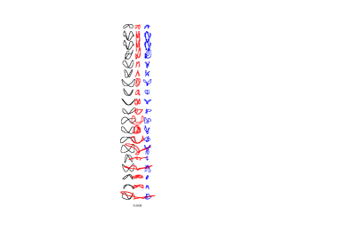
Figure 17: Quality of prediction on a reference data set. Cf. color code of Figure 12

9.2 Dynamic analysis

The comparison of Figure 14 and 15 is encouraging: when simulating exactly the system from which trajectories were aquired experimentally in the first place, the simulation come strickingly close to the experimental results. It is understood that a simulation is good if it captures the statistical properties of the real response. VIV being chaotic, there is no hope to reproduce exactly any given realization of the response.

Figure 16 shows the result of a simulation of a case which is also directly represented in the training data. The simulation fails, in the sense that IL and CF vibrations are simulated to occur at the same frequency. Two explanations are proposed:

The quality of the force prediction by the rotatron, illustrated in Figure 12 was declared “satisfactory”, but this constitutes only an observation that the fitting procedure is operating. On what criteria should one judge that the fit is adequate? When training was carried out, the average norm of the difference between training force and predicted force was found to be about 30% of the average norm. For a control group composed of data points from the same experimental database, but not used in training the perceptron, the same ratio was about 40%. These number are high, and can be reduced to some extend by increasing the number of hidden layers and of training iterations, but this was not found to yield better simulations. Further specialising the perceptron (by training it with data from test 2030) did not lead to successful simulations. One study which might help to understand the observations would be to find the corrective forces that need to be added to the forces predicted by the model, to force the simulation to track the motions observed during test 2030. This can be achieved using dynamic inverse FEM analysis [10, 11, 12].

Even if the above corrective forces were strictly zero, so that the model was accurately predicting forces for the riser motion from test 2030, this would not be sufficient to ensure that the simulation adequately mimics test 2030. A given trajectory could still have very different stability properties in the physical system and in the simulation. It could be that in the physical system, the trajectories follows the “bottom of a valley” while model renders it as the “crest of a mountain”. A measure of stability for this is the Lyapunov exponent [9, 20]. Procedures exist to compute Lyapunov exponents from experimental data, and this should be compared to Lyapunov exponents for the simulation.

9.3 Influence of $t_{w}$

One issue that was explored was the adequacy of $t_{w}$: The rotatron was trained with $t_{w}=5\cdot 10^{-5}$. This corresponds roughly to 1/4 of a cross-flow oscillation period in reduced scale for test 2370, and to a smaller fraction for other tests at lower current velocity. It could be argued that this fraction becoming too small could be the cause of the failure of analyzes at lower velocities (Figure 16). The rotatron was hence trained again using a suitably increased value of $t_{w}$ . This was done twice, once with the full training set and increase the number of Laguerre polynomials to $n=60$, and once with only the experimental data from lower currents, and an unchanged number of polynomials ($n=30$). Neither rotatrons allowed to perform a successful simulation for the lower current velocities.

9.4 Tension

In Figure 14, one can observe modulations of the positions of the vibration nodes (in particular on the cross-flow graph). One possible explanation for this would be that in the physical system, the tension is modulated by the vibration. This effect, if present, is not captured by the numerical model, which assumes constant tension. The method presented here is designed for use in a non-linear analysis. However in this research, time was saved by using a simpler linear structural model.

10 Conclusions

A model for the prediction of VIV forces given the history of velocity of a cylindrical cross section relative to the undisturbed fluid, has been developed. The model is closely relatied to Wiener-Laguerre filters: the recent history of velocity is represented by the coefficients of a Laguerre polynomial series. These coeffcients are then used to enter a memory-less non-linear interpolation function, in this case, a custom made neural network in which some relevant symmetry properties were “hard-wired”. The neural network was trained by using forces and displacements obtained in irregular forced motion tests on a short cylinder.

The proposed model operates in the time domain, making it well suited for integration into fully non-linear analyses with unsteady currents. It further deals with in-linea and cross-flow vibrations as one inseparable issue, which is arguably a necessity to improve on existing VIV models.

The model could provide a “good” reproduction of the forces in the training test, as well a “good” prediction of forces for “comparable” trajectories. Were the model was queried with trajectories very different from those present in the training data, the model gave very poor results - as can be expected. Due to the limited amount of experimental data available, the present model remains quite specialized to a limited number of situations. What remains unknown at this stage is the size of the training set, and of the neural network model, necessary to create a model with some pretention of generality.

In some in dynamic analyses of laboratory tests (NDP TN2030 and TN2430) with a long flexible riser, the numerical solution fell into an unphysical mode of vibration with the same frequency for in-line and cross flow vibration. On the other hand, for another case (TN2470), some unusually fine details were captured by the numerical model.

From this, it is concluded that the concept has merit and deserves to be pursued, acknowledging that more work is needed to arrive to a pratical engineering tool.

11 Acknowledgments

The author is indebted to Ida Aglen, Celeste Barnardo, Trygve Kristiansen, Carl Martin Larsen, Halvor Lie, Elizabeth Passano, Thomas Sauder, Wu Jie and Yin Decao for inspiring discussions on the subject of VIV, that either led to or helped the present research and writing. Thanks are extended to CeSOS (Centre of Excellence for Ships and Offshore Structures) at NTNU (Norwegian University of Science and Technology) and to MARINTEK for sponsoring this research. Very special thanks to Professor Carl Martin Larsen of CeSOS who, faced with a barrage of dubious ideas from the author, responded by making this research possible.

Appendix A Conventions for indexed notations

In the present work, index notations inspired from tensor analysis are used. However, the present setting differs from tensor analysis in at least three ways:

First, we assume that we are only operating in Euclidian spaces (an not in more general Riemannian manifolds) so that orthogonal bases can be used. This makes it unnecessary to distinguish between co- and contravariant bases and coordinates. Hence, only lowered indexes appear in the present work. Incidentally, it was here assumed that the state of the model is a point in a vector space, which is not true when finite rotations are present and Riemanian geometry should be introduced instead.

Second, in tensor notations, each index spans the dimension of the manifold. In an expression like $\sigma_{ij}=C_{ijkl}\;\varepsilon_{kl}$ the indices range from 1 to 3. Following Einstein’s convention, indices $k$ and $l$ are summed over, and the relation is valid for any combination of $i$ and $j$. The fact that the equation is valid at each point within a solid is implicit in the notation. In the present work we prepare for the manipulations of arrays in a computer, involving operations that are repeated, for example for various locations alomg a riser. If indexes $x$, $y$ and $z$ were introduced to note the position to which the various tensors refer, one would tend to write $\sigma_{ijxyz}=C_{ijklxyz}\;\varepsilon_{klxyz}$ , which violates Einstein’s convention, because no summation (or rather: no integral) is implied over the positions.

Third, we introduce non-linear functions. These functions can combine the values of the coordinates for some indices, and operate in parallel on the coordinates for other indices.

Hence the following conventions are used:

1. By default, where an index appears more than once in a combination of products and/or divisions, a summation over the index is implied. If that index has a continuous range, then the “sum” is an integration over the range. Point 2, 3 and 4 specify exceptions to this rule.

2. Point 1 notwithstanding, if an equation is preceded by the symbol $\forall$, followed by a list of indexes, then the listed indexes are not summed over.

3. Point 1 notwithstanding, if within an equation, there is a combination of products and/or divisions within which an index appears only once, then no sum over that index is carried out in the whole equation. (In any other situation than a simple term in the left hand side, readability should be improved by using the symbol $\forall$ . )

4. Point 1 notwithstanding, if an index appears within an input to a function, and the output of the function is multiplied or divided by one or several terms that have the same index, then no sum within the input to the function is carried out on that index.

5. If an index of an argument to a function is within brackets, then the whole range of index values is used as input to one function evaluation. For example, $\sigma_{i}\left(y_{[j]k}\right)$ refers to the evaluation a multiple locations ($k$) of a vector-valued ($i$) function of a vector ($j$).

6. When the output of the function is shorthanded without explicitly writing its input, then the indices of the input that are not within bracket are added to the indices of the function. For example $\sigma_{i}\left(y_{[j]k}\right)$ can be shorthanded $\sigma_{ik}$.

7. Derivatives of a function are noted with only the bracketed indices of the input appearing under the fraction: $\frac{\partial\sigma_{i}}{\partial y_{j}}$ . To refer to the value of that derivative for input $k$, one writes $\frac{\partial\sigma_{ik}}{\partial y_{j}}$ .

Appendix B Rotatron gradients

The derivative of the force predicted by the rotatron, with respect to the Laguerre coefficients is needed in Section 7. With references to Equations 64 to 69 that describe the rotatron, we can write

$$\frac{\partial\hat{f}_{in}}{\partial\dot{\tau}_{jl}} = \frac{\partial\hat{f}_{in}}{\partial\sigma_{k}}\frac{\partial\sigma_{ikn}}{\partial y_{j}}\frac{\partial y_{jkn}}{\partial\dot{\tau_{l}}}$$ (119)

$$= V_{k}\frac{\partial\sigma_{ikn}}{\partial y_{j}}M_{kl}$$ (120)

with

$$\frac{\partial\sigma_{ikn}}{\partial y_{j}}=-\frac{1}{\left|y_{[j]kn}\right|^{3}\left(\left|y_{[j]kn}\right|^{\alpha_{k}}+1\right)^{2}}\times\\ \left[\vphantom{\frac{a}{b}}\alpha_{k}\,y_{ikn\,}y_{jkn}\left|y_{[j]kn}\right|^{\alpha_{k}}\right.\\ \left.+(-1)^{\delta_{ij}}y_{\neg ikn\,}y_{\neg jkn}\left(\left|y_{[j]kn}\right|^{\alpha_{k}}+1\right)\vphantom{\frac{a}{b}}\right]$$ (121)

Here index $i$ ranges over two values (for two directions orthogonal to the cylinder), and $\neg i$ is the other direction than $i$.

The gradients of the rotatron with respect to its coefficients are also needed in order to compute the gradient of the target function with respect to the parameters $V_{k}$, $U_{k}$ and $M_{kl}$.

$$\frac{\partial\hat{f}_{in}}{\partial V_{l}} = \sigma_{iln}$$ (122)

$$\frac{\partial\hat{f}_{in}}{\partial M_{kl}} = \frac{\partial\hat{f}_{in}}{\partial\sigma_{k}}\frac{\partial\sigma_{ikn}}{\partial y_{j}}\frac{\partial y_{jkn}}{\partial M_{kl}}$$ (123)

$$= V_{k}\frac{\partial\sigma_{ikn}}{\partial y_{j}}\dot{\tau}_{jln}$$ (124)

$$\frac{\partial\hat{f}_{in}}{\partial U_{l}} = V_{k}\frac{\partial\sigma_{ikn}}{\partial U_{l}}$$ (125)

with

$$\frac{\partial\sigma_{ikn}}{\partial U_{l}}=-\delta_{kl}\frac{e^{-U_{l}}y_{ikn}\left|y_{[j]kn}\right|^{\alpha_{k}-1}\log\left|y_{[j]kn}\right|}{\left(\left|y_{[j]kn}\right|^{\alpha_{k}}+1\right)^{2}}$$ (126)

Appendix C Inverse of $s5$

The inverse of $s5$ (Equation 109), where $s5$ is of the form

$$s5_{ij}=\alpha T_{ij}+\beta\delta_{ij}$$ (127)

with

$$\begin{cases}T_{ij}=1&\quad j\leq i\\ \phantom{T_{ij}}=0&\quad j>i\end{cases}$$ (128)

can be verified to be lower triangular banded, with terms on diagonal $i$ equal to

$$Q_{1} = \frac{1}{\alpha+\beta}$$ (129)

$$Q_{i} = -\frac{\alpha\beta^{i-2}}{\left(\alpha+\beta\right)^{i}}\quad i\in\left\{2\dots n\right\}$$ (130)

References

- [1] Milton Abramowitz and Irene A. Stegun. Handbook of Mathematical Functions with Formulas, Graphs, and Mathematical Tables. Dover, New York, ninth dover printing, tenth GPO printing edition, 1964.
- [2] S. Chen and S.A. Billings. Neural networks for nonlinear system modeling and identification. International Journal of Control, 56(2):pp. 319 –346, 1992.
- [3] Henning Braaten et al. NDP riser high mode VIV tests - Main report, MT51 F05-072. Technical report, MARINTEK, 2005.
- [4] M. L. Facchinetti, E. de langre, and F. Biolley. Coupling of structure and wake oscillators in vortex induced vibrations. Journal of fluids and structures, x:x, 2003.
- [5] Odd M. Faltinsen. Sea loads on ships and offshore structures. Cambridge University Press, 1990.
- [6] Lyle Finn, Kostas Lambrakos, and Jim Maher. Time domain prediction of riser viv. In 4th international conference on advances in riser technology, Aberdeen, 1999.
- [7] Kenneth Levenberg. A method for the solution of certain non-linear problems in least squares. The Quarterly of Applied Mathematics, 2:pp. 164 – 168, 1944.
- [8] Halvor Lie. A time domain model for simulation of vortex induced vibrations on a cable. In Bearman, editor, Flow induced vibration, pages pp. 455 – 466. Balkema, 1995.
- [9] Aleksandr Lyapunov. General problem of the stability of motion. PhD thesis, Moscow University, 1892.
- [10] P. Mainçon. Inverse finite element methods – part I: Estimating loads and structural response from measurements. In A. Zingoni, editor, SEMC 2004, 2004.
- [11] P. Mainçon. Inverse finite element methods – part II: Dynamic and non-linear problems. In A. Zingoni, editor, SEMC 2004, 2004.
- [12] Philippe Mainçon, Celeste Barnardo, and Carl Martin Larsen. VIV force estimation using inverse FEM. In OMAE, 2008.
- [13] B. B. Mandelbrot. How long is the coast of britain. statistical self similarity and fractional dimension. Science, 156:pp. 636 – 638, 1967.
- [14] Donald Marquardt. An algorithm for least-squares estimation of nonlinear parameters. SIAM Journal on Applied Mathematics, 11:pp. 431 – 441, 1963.
- [15] L. Mathelin and E. de Langre. Vortex-induced vibrations and waves under shear flow with a wake oscillator model. European Journal of Mechanics, 24:pp. 478 – 490, 2005.
- [16] Martin Fodslette Møller. A scaled conjugate gradient algorithm for fast supervised learning. Neural networks, 6:pp. 525 – 533, 1993.
- [17] J. R. Morison, M. P. O’Brien, J. W. Johnson, and S. A. Schaaf. The force exerted by surface waves on piles. Petroleum Transactions (American Institute of Mining Engineers), 189:pp. 149 – 154, 1950.
- [18] Benjamin Muckenhoupt. Mean convergence of Hermite and Laguerre series. II. Transactions of the American Mathematical Society, 147(2):pp. 433–460, 1970.
- [19] J. A. Nelder and R. Mead. A simplex method for function minimization. Computer Journal, 7:pp. 308 – 313, 1965.
- [20] Edward Ott. Chaos in dynamical systems. Cambridge University Press, 2002.
- [21] Raul Rojas. Neural Networks - A Systematic Introduction. Springer-Verlag,, Berlin, New-York,, 1996.
- [22] Frank Rosenblatt. The perceptron: A probabilistic model for information storage and organization in the brain. Cornell Aeronautical Laboratory, Psychological Review, 65(6):pp. 386–408, 1958.
- [23] J. Sjöberg and L. Ljung. Overtraining, regularization, and searching for minimum in neural networks. In In Preprint IFAC Symposium on Adaptive Systems in Control and Signal Processing, pages pp. 669 – 674, 1992.
- [24] R. Violette, E. de Langre, and J. Szydlowski. Computation of vortex-induced vibrations of long structures using a wake oscillator model: Comparison with dns and experiments. Computers and structures, 85:pp. 1134–1141, 2007.
- [25] Remi Violette. Modele lineaire des vibrations induites par vortex de structures elancees. PhD thesis, Ecole Polytechnique, 2009.
- [26] Norbert Wiener. Nonlinear problems in random theory. The Technology Press of Massachusetts Institute of Technology, 1958.