Accurate and efficient algorithm for Bader charge integration

Abstract

We propose an efficient, accurate method to integrate the basins of attraction of a smooth function defined on a general discrete grid, and apply it to the Bader charge partitioning for the electron charge density. Starting with the evolution of trajectories in space following the gradient of charge density, we derive an expression for the fraction of space neighboring each grid point that flows to its neighbors. This serves as the basis to compute the fraction of each grid volume that belongs to a basin (Bader volume), and as a weight for the discrete integration of functions over the Bader volume. Compared with other grid-based algorithms, our approach is robust, more computationally efficient with linear computational effort, accurate, and has quadratic convergence. Moreover, it is straightforward to extend to non-uniform grids, such as from a mesh-refinement approach, and can be used to both identify basins of attraction of fixed points and integrate functions over the basins.

I Introduction

Based on density functional theory (DFT)Kohn and Sham (1965) calculations, decomposing the charge or the energy of a material into contributions from individual atoms can provide new information for material properties. Bader’s “atoms in molecules” theory provides an example of a partitioning based on the charge density, and following the gradient at a particular point in space to the location of a charge density maximum centered at an atom—defining basins of attraction of fixed points of the charge density. Bader defines the atomic charges and well-defined kinetic energies as integrals over these Bader volumes,Bader (1990) $\Omega_{\rho}$. Each Bader volume contains a single electron density maximum, and is separated from other volumes by a zero flux surface of the gradients of the electron density, $\nabla\rho(\vec{r})\cdot\hat{n}=0$. Here, $\rho(\vec{r})$ is the electron density, and $\hat{n}$ is the unit vector perpendicular to the dividing surface at any surface point $\vec{r}\in\partial\Omega_{\rho}$. Each volume $\Omega_{\rho}$ is defined by a set of points where following a trajectory of maximizing $\rho$ reaches the same unique maximum (fixed point). In practical numerical calculations, where the charge density is defined on a discrete grid of points in real space, it is very challenging to have an accurate determination of a zero flux surface.

Different approaches for condensed, periodic systems have relied on analytic expressions of the densityBiegler-König et al. (1981); Popelier (1996) or discretizing the charge density trajectoriesMalcolm and Popelier (2003); Uberuaga et al. (1999); Henkelman et al. (2006); Tang et al. (2009); Otero-de-la-Roza and Luaña (2010). Early algorithms were based on the electron density calculated from analytical wavefunctions of small molecules, and integration along the gradient paths. Most current developments are based on a grid of electron density, which is important for DFT calculation and also applicable to analytical density function of small molecules. One octal tree algorithmMalcolm and Popelier (2003) uses a recursive cube subdivision to find the atomic basins robustly, but practically is not applicable to complicated topologies due to huge computational cost. The “elastic sheet” methodUberuaga et al. (1999) defines a series of fictitious particles which gives a discrete representation of zero-flux surface. Particles are relaxed according to the gradients of charge density and interparticle forces. This method will not work for complex surface with sharp cusps or points. Recently, Henkelman et al. developed an on-grid methodHenkelman et al. (2006) to divide an electron density grid into Bader volumes. This method can be applied to the DFT calculations of large molecules or materials. They discretize the trajectory to lie on the grid, ending at the local maximal point of the electron density. The points along each trajectory are assigned to the atom closest to the end point. Although this method is robust, and scales linearly with the grid size, it introduces a lattice bias caused by the fact that ascent trajectories are constrained to the grid points. The near-grid methodTang et al. (2009) improves this by accumulating a correction vector—the difference between the discretized trajectory and the true trajectory—at each step. When the correction vector is sufficiently large, the discrete trajectory is corrected to a neighboring grid point. This method corrects the lattice bias, and also scales linearly with respect to the size of grids. However, both grid trajectory methods require iteration to self-consistency in volume assignments. Also, the integration error scales linearly with the grid spacing, so very fine grids are required in numerical calculations to provide the correct Bader volume, reducing its applicability for accurate calculations in a large system. Lastly, a new algorithm uses a “divide and conquer” adaptive approach with tetrahedra; tetrahedra are continuously divided at the boundaries of Bader volumes, with the weight of each tetrahedra given by the number of vertices that belong to each volumeOtero-de-la-Roza and Luaña (2010). Such an approach retains linear scaling with the grid spacing, but requires mesh refinement near boundaries to deal with the linear convergence of the error with the grid spacing.

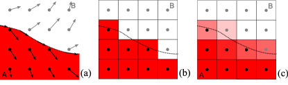
Figure 1: A schematic illustration of the zero flux surface, the near-grid algorithm, and weighted integration. The zero flux dividing surface separate volumes A and B, where arrows denote charge density gradients (a). The normal component is zero for any point on the surface $\nabla\rho\cdot\hat{n}=0$. The near-grid methodTang et al. (2009) gives grid-based partition (b), however energy density integration based on this grid-based partition would cause integration error due to finite grid sizes. A weight function (c) representing volume fractions of the cell of each grid point is introduced to reduce the error due to a finite grid.

Figure 1 illustrates the partition of the real space into two Bader volumes A and B by a zero flux dividing surface. The component of $\nabla\rho$ along the surface normal $\hat{n}$ is zero for any point on the surface $\partial A$ or $\partial B$. A grid-based partition algorithm, such as the near-grid method, divides space into volume surrounding around each grid point, and assigns each grid volume to a particular Bader volume. Even though grid points may be assigned to Bader volumes correctly, the density integration based on the grid-based partition would bring in numerical integration error that scales linearly with the grid spacing. Introducing a “weight” integrand representing the fraction of grid volume that belongs to a particular Bader volume smooths out the grid-based partition, and improves the integration accuracy and scales quadratically with the grid spacing. The atomic contribution is neither 1 nor 0 at the dividing surfaces, but fractional. In Figure 1, red represents a weight of 1 to atom A for grid points closer to atom A, and transitions to white for a weight of 0 for grid points away from atom A.

The grid-based weight representing volume fractions of each grid volume assigned to different atoms, and gives a more accurate integrand for the integration of either charge density or of kinetic energy over the Bader volumes. The weight is computed from the total integrated flux of trajectories in a grid volume to neighboring grid volumes. The algorithm is robust, efficient with linear computing time in the number of grid points, and more accurate than other grid-based algorithm. Surprisingly, it combines both better error scaling—quadratic in the grid spacing—and improved computational efficiency. Moreover, it is straightforward to apply to nonuniform grids, such as would result from an adaptive mesh-refinement approach. In Section II, we derive the algorithm to constructing a grid-based weight to perform numerical integrals over Bader volumes. Section III presents examples including three dimensional charge density from three Gaussian functions in FCC cell, TiO₂ bulk, and NaCl crystal. Finally, we show the improved computational efficiency in Section IV. The end result is a simple, extendable, computationally efficient algorithm with quadratic integration error.

II The Weight Method

The Bader partitioning of space defines volumes by the endpoint of a trajectory following the gradient flow of the charge density, $\nabla\rho$. We assume that $\rho$ has continuous first and second derivatives throughout all space of interest, and has a set of discrete local maxima (fixed points) $\vec{x}_{1}$, $\vec{x}_{2}$, etc., where $\nabla\rho=0$ and the matrix $\nabla\nabla\rho$ is negative-definite. The basin of attraction $A_{n}$, of a fixed point $\vec{x}_{n}$ is the set of points which flow to the fixed point $\vec{x}_{n}$ along the charge density gradient. That is, for any point $\vec{r}$, we can integrate the trajectory given by $\dot{\vec{x}}(t)=\nabla\rho(\vec{x})$, with the initial condition $\vec{x}(0)=\vec{r}$, to find $\lim_{t\to\infty}\vec{x}(t)$. Each trajectory will end at fixed point $\vec{x}_{n}$, and except for a set of points with zero volume in space, the extremum is a local maximum; the basin of attraction $A_{n}$ are all points $\vec{r}$ whose trajectory $\lim_{t\to\infty}\vec{x}(t)$ ends at $\vec{x}_{n}$. Note also that if point $\vec{r}_{0}\in A$, and the trajectory starting from $\vec{r}_{1}$ reaches $\vec{r}_{0}$ in a finite time $t$, then $\vec{r}_{1}\in A$. This set defines a partitioning of space, where $A_{n}\cap A_{m}=\emptyset$ when $n\neq m$ and $\cup_{n}A_{n}=\Omega$. Finally, each basin $A_{n}$ is such that wherever the normal $\hat{n}$ to the bounding surface $\partial A_{n}$ is well-defined, $\hat{n}\cdot\nabla\rho=0$. If $\rho$ is the charge density, then $A_{n}$ are the Bader volumes; but this definition is applicable to any sufficiently smooth function with a discrete set of local maxima. As the definition of the basins $A_{n}$ derives from trajectories, it is not possible in general to determine if two neighboring points $\vec{r}$ and $\vec{r}^{\prime}$ belong to the same or different basins based only on local information.

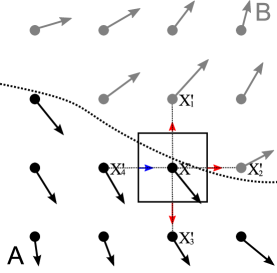
Figure 2: Schematic illustration of the weight method. The volume of the cell of a grid point flows to its neighbors with larger charge density magnitude. Flowing flux is shown as directional map, either flowing from $X$ to $X^{\prime}$ as red arrows or flowing from $X^{\prime}$ to $X$ as blue arrows.

Figure 2 shows the reformulation for an approximate fractional partitioning of real-valued function evaluated at a set of discrete points, $X$. The grid points $X$ partition space into Voronoi polyhedraVoronoi (1907) $V_{X}$ covering each grid point $X$, where a point in space $\vec{r}$ belongs to the volume $V_{X}$ if $X$ is the closest point in Cartesian space to $\vec{r}$. Each polyhedra is defined by the nearest neighboring points $X^{\prime}$ that are a distance $\ell_{X\to X^{\prime}}$ away; the Voronoi polyhedron at $X$ has facets $\partial V_{X\to X^{\prime}}$ with normal $\hat{n}_{X\to X^{\prime}}$ pointing from $X$ to $X^{\prime}$ and area $a_{X\to X^{\prime}}$. Moreover, the facet is at the midpoint between $X$ and $X^{\prime}$. Our goal is to define for each grid point $X$, a “weight” $w^{A}(X)$ between 0 and 1 such that $\sum_{A}w^{A}(X)=1$ for all $X$, and the discrete approximation to the integral over the basin $A$

$$\int_{A}d^{3}rf(\vec{r})\approx\sum_{X}V_{X}w^{A}(X)f(X)$$ (1)

converges quadratically in the grid spacing for smooth functions $f(\vec{r})$. The weight, in this case, is the fraction of points in $V_{X}$ whose trajectory ends in the basin $A$. Note that if the points $X$ form a regular periodic grid, the Voronoi volumes, facet areas, and neighbor distances need only be computed for the Wigner-Seitz cell around a grid point.

To transition from the continuum definition of spatial partitioning to our Voronoi partitioned definition, we introduce the continuum probability density for our trajectories, $P(\vec{r},t)$. From the trajectory equation, the probability flux at any point and time is $\vec{j}(\vec{r},t)=P(\vec{r},t)\nabla\rho(\vec{r})$. Then, the probability distribution evolves in time according to a continuity equation

$$\frac{\partial P(\vec{r},t)}{\partial t}+\nabla\cdot(P(\vec{r},t)\nabla\rho(\vec{r}))=0.$$ (2)

This equation represents the combined evolution of a distribution of points in space; we use it to determine how the points in $V_{X}$ distribute to neighboring volumes $V_{X^{\prime}}$. Define the volume probability

$$P_{X}(t)=V_{X}^{-1}\int_{V_{X}}d^{3}rP(\vec{r},t);$$ (3)

then the evolution from the initial condition

$$P(\vec{r},0)=\begin{cases}1&:\vec{r}\in V_{X}\\ 0&:\vec{r}\notin V_{X}\end{cases}$$ (4)

is given by

$$\begin{split}\frac{dP_{X}(t)}{dt}&=-V_{X}^{-1}\int_{V_{X}}d^{3}r\nabla\cdot(P(\vec{r},t)\nabla\rho(\vec{r}))\\ &=-V_{X}^{-1}\sum_{X^{\prime}}\int_{\partial V_{X\to X^{\prime}}}P(\vec{r},t)\nabla\rho\cdot\hat{n}_{X\to X^{\prime}}d^{2}r\\ &\approx-V_{X}^{-1}P_{X}(t)\sum_{X^{\prime}}\int_{\partial V_{X\to X^{\prime}}}\nabla\rho\cdot\hat{n}_{X\to X^{\prime}}d^{2}r\\ &\approx-P_{X}(t)\sum_{X^{\prime}}\frac{a_{X\to X^{\prime}}}{V_{X}}\cdot\frac{R(\rho_{X^{\prime}}-\rho_{X})}{\ell_{X\to X^{\prime}}}\\ &\equiv-P_{X}(t)\sum_{X^{\prime}}\tau_{X\to X^{\prime}}\end{split}$$ (5)

where $R(u)=u\theta(u)$ is the ramp function, so that $\tau_{X\to X^{\prime}}\geq 0$ and is zero when $\rho_{X^{\prime}}<\rho_{X}$; this is a consequence of our initial conditions where $P(r,0)$ is only nonzero in the interior of $V_{X}$. The first approximation ignores spatial variation of $P(r,t)$ through the volume $V_{X}$ (an error linear in the grid spacing), and the second approximation ignores spatial variation of $\nabla\rho$ along a facet $\partial V_{X\to X^{\prime}}$, and approximates the gradient at the midpoint between $X$ and $X^{\prime}$ with the finite difference value (also with an error that is linear in the grid spacing). The solution to Eqn. 5 is $P_{X}(t)=\exp(-t\sum_{X^{\prime}}\tau_{X\to X^{\prime}})$. For that solution, the time-integrated flux of probability from $V_{X}$ to $V_{X^{\prime}}$ through the facet $\partial V_{X\to X^{\prime}}$ is

$$\begin{split}J_{X\to X^{\prime}}&=\int_{0}^{\infty}dt\int_{\partial V_{X\to X^{\prime}}}P(\vec{r},t)\nabla\rho\cdot\hat{n}_{X\to X^{\prime}}d^{2}r\\ &\approx\int_{0}^{\infty}dtP_{X}(t)\int_{\partial V_{X\to X^{\prime}}}\nabla\rho\cdot\hat{n}_{X\to X^{\prime}}d^{2}r\\ &\approx\int_{0}^{\infty}dtP_{X}(t)\tau_{X\to X^{\prime}}\\ &=\frac{a_{X\to X^{\prime}}\ell_{X\to X^{\prime}}^{-1}R(\rho_{X^{\prime}}-\rho_{X})}{\sum_{X^{\prime}}a_{X\to X^{\prime}}\ell_{X\to X^{\prime}}^{-1}R(\rho_{X^{\prime}}-\rho_{X})}\end{split}$$ (6)

where we have used the same approximations as above. This flux defines the total fraction of points inside $V_{X}$ that transition to volume $V_{X^{\prime}}$ through $\partial V_{X\to X^{\prime}}$. Note that $\sum_{X^{\prime}}J_{X\to X^{\prime}}=1$, unless $X$ is a local (discrete) maxima, where $\rho_{X}>\rho_{X^{\prime}}$ for all neighbors $X^{\prime}$. Finally, as the weight $w^{A}(X)$ represents the volume fraction of points in volume $V_{X}$ whose trajectory ends inside basin $A$, then

$$w^{A}(X)=\sum_{X^{\prime}}J_{X\to X^{\prime}}w^{A}(X^{\prime}).$$ (7)

Note that if for all $X^{\prime}$ where $\rho(X^{\prime})>\rho(X)$, $\sum_{A}w^{A}(X^{\prime})=1$, then as $\sum_{X^{\prime}}J_{X\to X^{\prime}}=1$, Eqn. 7 guarantees that $\sum_{A}w^{A}(X)=1$. Appendix A shows that the error in the weight of linear order in the grid spacing produces a quadratic order error in the integration.

Forward substitution solves Eqn. 7 after the grid points are sorted from highest to lowest density $\rho(X)$. Sequentially, each point $X$ is either

1. A local maxima: $\rho(X)>\rho(X^{\prime})$ for all neighbors $X^{\prime}$. This grid point corresponds to a new basin $A$, and we assign $w^{A}(X)=1$.

2. An interior point: for all $X^{\prime}$ where $\rho(X^{\prime})>\rho(X)$, the weights have been assigned and $w^{A}(X^{\prime})=1$ for the same basin $A$. Then Eqn. 7 assigns $X$ to basin $A$ as well: $w^{A}(X)=1$.

3. A boundary point; with weights between 0 and 1 for multiple basins assigned by Eqn. 7.

Then $w^{A}(X)$ is known from $w^{A}(X^{\prime})$ where $\rho(X^{\prime})>\rho(X)$ for each basin $A$ (as $J_{X\to X^{\prime}}\neq 0$ only if $\rho(X^{\prime})>\rho(X)$). Note also that the weight for a particular basin $A_{n}$ is assigned without reference to any other basin $A_{m}$; once the set of time-integrated fluxes $J_{X\to X^{\prime}}$ are known and the densities sorted in descending order, the solution for each basin is straightforward, and Eqn. 7 is only needed on the boundary points.

This algorithm solves several issues with the near-grid method. It requires no self-consistency, which improves the computational scaling. Moreover, the introduction of smooth functions that define the volume fraction of points in each basin produces less error and faster convergence with additional grid points. The algorithm is also readily applicable to non-uniform grids, such as an adaptive meshing scheme—it only requires computation of the Voronoi volumes and facets for the grid points. In one dimension, Eqn. 1 has quadratic convergence in the grid spacing (c.f. Appendix A); we now demonstrate the quadratic convergence and improved integration accuracy for three dimensional problems.

III Evaluation of numerical convergence

One determination of the accuracy of Bader volume integration is the vanishing of the volume integration of the Laplacian of charge density $\nabla^{2}\rho(\mathbf{r})$. The non-zero value of the Laplacian of charge density integration within each Bader volume is our atomic integration error, and can be used as an estimate of the error of the integration of the kinetic energy. We construct the zero flux surface of the gradients of charge density and evaluate the integration error with both the weight- and near-grid methods for several cases. First, we consider an analytic charge density with known boundaries in an orthogonal and a non-orthogonal cell. Next, we calculate real systems: an ionic compound, and a semiconductor. We also evaluate the Bader charge of Na atom in NaCl crystal by integrating the charge density within Bader volume, and compare the convergence with the near-grid method.

III.1 Gaussian densities

Figure 3 shows an example of misassignment of the grid points to basins from the near-grid method. Misassignment occurs for the grid points close to the dividing surfaces with the gradients of charge density almost parallel to the surfaces. In this example, a three dimensional model charge density is constructed from three Gaussian functions in simple cubic unit cell, $\rho(\vec{r})=\sum_{i=1,3}e^{(-\vec{r}-\vec{r}_{i})^{2}/W^{2}}$. The $\vec{r}_{i}$ are $(0.25N,0.25N,0.4N)$, $(0.5N,0.5N,0.5N)$, and $(0.75N,0.75N,0.4N)$, with width $W=N/10$. Figure 3 shows the charge density distribution on $(1\bar{1}0)$ plane. Due to the symmetry of charge density distribution, the true dividing surfaces along charge density saddle points are known analytically and shown as two black lines on $(1\bar{1}0)$ plane. The grid points marked by orange circles are assigned to the wrong basins by the near-grid method, different from the partition of spatial points by true dividing surfaces. The gradients of charge density shown in arrows for these misassigned surface points have small normal components, and we believe this is the cause of the misassignment.

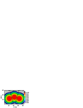
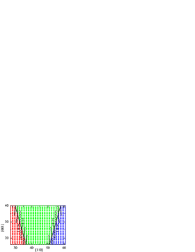
Figure 3: Charge density distribution constructed from three Gaussian functions, and basin identification with near-grid and the weight method. The grid size is $N=60$, and the charge density is shown on $(1\bar{1}0)$ plane; this is coplanar with the centers of the three Gaussian functions. The true dividing surfaces are indicated by two black lines due to symmetry. The basin assignment of grid points is given: red dots for ion I, green dots for ion II, and blue dots for ion III; for the weight method, a single color is assigned to the maximum weight at each point. Basin assignment from the near-grid method is given in the middle panel; basins with maximal weight on every grid points from the weight method are indicated in the right panel. Orange circles in the middle panel indicate the grid points misassigned by the near-grid method and corrected by the weight method. Arrows in the bottom panel denote the directions of the gradients of charge density, which can be used to verify the correctness of basin assignment.

To test integration accuracy beyond simple cubic lattices, we map this model charge density onto a FCC unit cell shown in Figure 4. The three dimensional model charge density is constructed from three Gaussian functions, $\rho(\mathbf{r})=\sum_{i=1,3}e^{(-\mathbf{r}-\mathbf{r}_{i})^{2}/W^{2}}$. The $\mathbf{r}_{i}$ are located at $(0.25N,0.25N,0.4N)$; $(0.5N,0.5N,0.5N)$; $(0.75N,0.75N,0.4N)$ where $N^{3}$ is the number of grid points in the FCC unit cell and $W=N/10$. We vary $N$ from 20 to 100. The Voronoi cell of FCC lattice has 12 neighbors, where all facets have the same area. The atomic weights on every grid represents the fraction of Voronoi volume of that grid point flowing to specific atom through its neighbors. By calculating on a set of grid sizes, one obtains the maximal atomic integration errors from the near-grid method and the weight method.

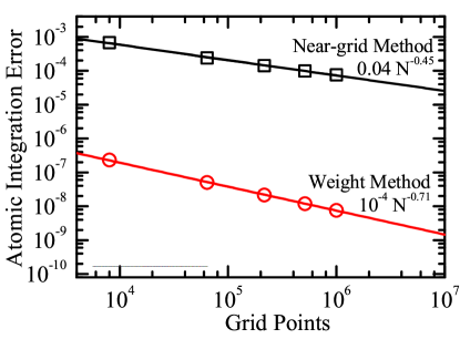
Figure 4: Comparison of the near-grid method and the weight method on atomic integration errors in a FCC cell. The maximal atomic volume integrations of the Laplacian of charge density within Bader volumes using the near-grid method and the weight method are denoted by squares and circles, respectively. We calculate charge density grids ranging from $20^{3}$ points to $100^{3}$. Our algorithm gives atomic integration errors three orders of magnitude lower than the near-grid method, and converges faster than the near-grid method.

Figure 4 shows a reduction in error of three orders of magnitude from the near-grid method. Fitting data to a non-linear function $y=a\,N^{-r}$ gives a convergence rate of 0.71 for the weight method, and 0.45 for the near-grid method. The exponent of 0.71 is close to the 2/3 expected for quadratic convergence, and 0.45 is close to the 1/3 expected for linear convergence. The weight method has both better absolute error and converges faster than the near-grid method; in addition, there is no crossover point at large grid spacing where near-grid has smaller errors.

III.2 Titania bulk

For a real charge density, we perform DFT calculations on TiO₂ bulk by use of the projector augmented wave (PAW)Blöchl (1994) method, the GGA with PBE functionalPerdew et al. (1996) for the exchange-correlation energy. Density-functional theory calculations are performed with vaspKresse and Hafner (1993); Kresse and Furthmüller (1996) using a plane-wave basis with the projector augmented-wave (PAW) method,Blöchl (1994) with potentials generated by Kresse.Kresse and Joubert (1999) Atomic configurations for Ti and O are [Ne]$3s^{2}3p^{6}4s^{2}3d^{2}$ with cutoff radius 1.22Å, and [He]$2s^{2}2p^{4}$ with cutoff radius 0.58Å, respectively. We use a plane-wave basis set with cut-off energy of 900eV. The tetragonal unit cell of rutile TiO₂ (see Figure 5) contains two Ti atoms and four O atoms. Monkhorst-Pack k-point method with $4\times 4\times 6$ k-points for six-atom cell is used for Brillouin-zone integration with a Gaussian smearing of 0.1eV for electronic occupancies. Theoretically optimized lattice constant are $a=4.649\text{\AA}$, $c=2.970\text{\AA}$, $u=0.305$ agreeing with experimental lattice constants of $a=4.584\text{\AA}$, $c=2.953\text{\AA}$, $u=0.305$Diebold (2003). A set of charge density grids ranging from $45\times 45\times 30$, $60\times 60\times 40$, $75\times 75\times 50$, $90\times 90\times 60$, $120\times 120\times 80$ points to $150\times 150\times 100$ are calculated. For the energy cutoff of 900eV, a grid of $45\times 45\times 30$ is required to eliminate wrap-around errors, and is the minimum size used by an accurate vasp calculation.

Figure 5 shows maximal atomic integration errors as a function of grid sizes. The weight method gives maximal atomic integration error one order of magnitude lower than the near-grid method systematically. The atomic integration error larger than 1.0eV on the minimal grid size $45\times 45\times 30$ from the near-grid method is unacceptably large. Again, the convergence rate of the error goes as $\sim 2/3$ for the weight method—corresponding to quadratic convergence—and $\sim 1/3$ for the near-grid method—corresponding to linear convergence. Both the improved error and faster convergence allows for more accurate density integration with fewer grid points than near-grid.

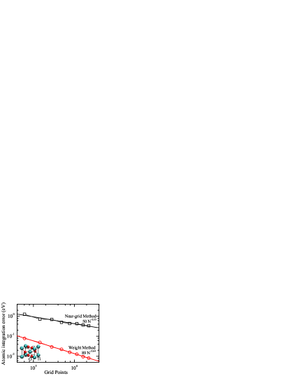
Figure 5: Maximal atomic integration error on rutile TiO₂ with respect to the charge density grids. A set of charger density grids ranging from $45\times 45\times 30$ points to $150\times 150\times 100$ points are calculated. The weight method reports maximal atomic integration error at least one order of magnitude smaller than the near-grid method. The weight method is practically useful for calculation of small grid size.

III.3 NaCl crystal

In this example, we evaluate the Bader charge (valence electron density integration within Bader volume) of Na atom in NaCl crystal by integrating the charge density within Bader volume, and compare the value with the near-grid method. We perform DFT calculations by use of the PAW method, the GGA with PW91 functionalPerdew and Wang (1992) for the exchange-correlation energy. Atomic configurations for Na and Cl are [He]$2s^{2}2p^{6}3s^{1}$ with cutoff radius $0.77\,\text{\AA}$, and [Ne]$3s^{2}3p^{5}$ with cutoff radius $1.00\,\text{\AA}$, respectively. A plane-wave basis set with cut-off energy of 500eV is applied. The NaCl unit cell contains 4 Na atoms and 4 Cl atoms. Monkhorst-Pack k-point method with $3\times 3\times 3$ k-points for eight-atom cell is used for Brillouin-zone integration with a Gaussian smearing of 0.2eV for electronic occupancies. The optimized lattice constant of 5.67Åagrees with the experimental lattice constant of 5.64Å. A set of charge density grids of $60^{3}$, $80^{3}$, $100^{3}$, $120^{3}$, to $180^{3}$ points are calculated.

Figure 6 shows the maximal atomic integration error as a function of various grid sizes. The weight method again shows maximal atomic integration error at least one order of magnitude lower than the near-grid method systematically. The scaling of the error goes as the $\sim 2/3$ power for the weight method, showing continued quadratic convergence, while the near-grid method error scales as the $\sim 1/3$ power, which is linear convergence.

Figure 7 shows that Bader charge of Na atom evaluated on various charge grids. The weight method computes a Bader charge of Na atom slightly larger than the near-grid method. Fitting the data to $\rho=\rho_{0}+\frac{C}{N_{grid}^{\alpha}}$, we find converged Bader charge values of $0.878$e, $0.881$e, for the near-grid method and the weight method, respectively. We believe this is due to a systematic misassignment for the near-grid method, as shown for the Gaussian charge density case. This suggests that the misassignment may not be improved by increasing the density of grid points in the near-grid method. This suggests that a “divide and conquer” approach using continually refined grids can face potential difficulty. For $60^{3}$ grid points, the near-grid method underestimates the Bader charge by 0.01e, while the weight method underestimates it by 0.005e, again showing faster convergence.

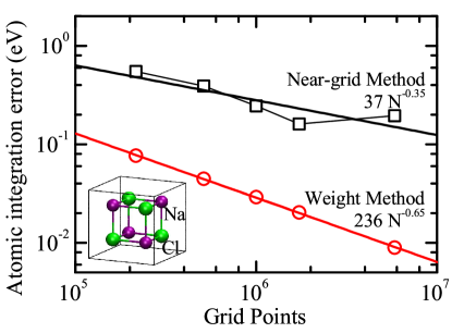
Figure 6: Comparison of the near-grid method and the weight method for maximal atomic integration error of NaCl crystal. A set of charge density grids ranging from $60^{3}$ points to $180^{3}$ points are calculated. Comparing to the near-grid method, the weight method reduce the integration error remarkably.

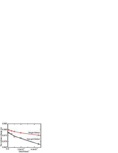
Figure 7: Comparison of the near-grid method and the weight method on convergence of Bader charges of Na in NaCl crystal. The Bader charge of Na is calculated for a set of density grids ranging from $60^{3}$ points to $180^{3}$ points. Both methods give monotonic, and smooth convergence.

IV Computational effort

The weight method is computationally efficient, requiring overall effort that scales linearly with the number of grid points. The total computer time is comprised of two primary tasks: the sorting of charge density costs $O(N\log N)$ with $N$ grid points, and the atomic weight evaluation on the sorted grid points beginning from grid point with maximum density requires at most $N\times N_{\text{atom}}$ computer time. The computational effort is smaller than that, as only the surface grid points which have fractional atomic weights require $N_{\text{atom}}$ calculations, while each interior grid point require only one calculation. Generally, the number of surface grid points is a small fraction of the number of total grid points, and scales as $N^{2/3}$. For example, the ratio of the number of surface grid points to the number of total grid points is $14\%$ in NaCl crystal with total grid sizes $60^{3}$.

In a calculation with charge density grid sizes approaching $10^{7}$–$10^{8}$ grid points and up to hundreds of atoms in large supercells, we find our algorithm is not only more accurate, but more efficient than the near-grid method. Both methods scale linearly with the number of grid points. Figure 8 shows the linear scaling of computer time required to analyze the charge density grid for an eight-atom NaCl with the number of grid points. The improved efficiency of our algorithm appears to originate from the lack of a self-consistent refinement of basin assignment. Comparing to the near-grid method, which needs refinement integration, our weight method has small prefactor, although both are linearly scaled.

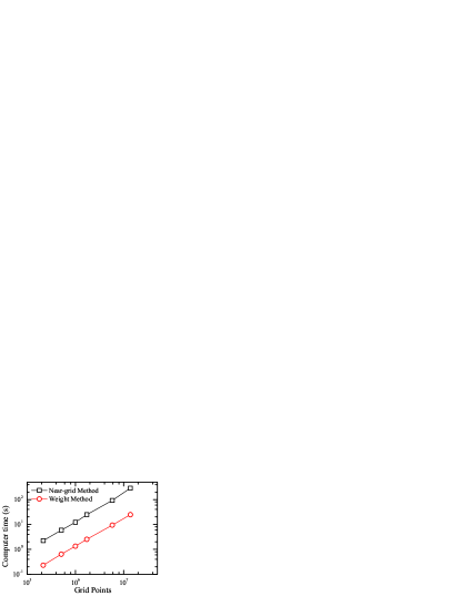
Figure 8: Computer time required to analyze the charge density grid for an eight-atom NaCl cell. The calculations were performed using an Intel Core2 Quad CPU Q6600, with a clockspeed of 2.40GHz. The computer time scales linearly with respect to the number of charge density grid sizes with the weight method, as with the near-grid method. The weight method has a smaller prefactor than the near-grid method.

V Conclusions

We develop a weight method to integrate functions defined on a discrete grid over basins of attraction (such as Bader volumes) in an efficient and accurate manner. The weight method works with the density on a discrete grid and assigns volume fractions of the Voronoi cell of each grid point to surrounding basins. Starting from the local density maxima, all the grid points are sorted in density descending order. Grid points can then be fractionally weighted from the weights of its neighbors with larger density. This method depends upon the formulation of flow across that dividing surfaces between the cells of two neighboring grid points, and can be applied to uniform or non-uniform grids.

We perform tests on model three-dimensional charge density constructed from Gaussian functions in FCC cell. The weight method shows that the atomic integration error is inversely proportional to the 2/3 power of grid points, while the integration error is inversely proportional to the 1/3 power of grid points using the near-grid method. We also perform tests on more realistic systems, such as TiO₂ bulk and NaCl crystal. In both cases, the weight method reports maximal atomic integration error at least one order of magnitude smaller than the near-grid method systematically. Furthermore, we calculate the Bader charge of NaCl crystal using these two methods, both give monotonic, and smooth convergence with respect to the increasing grid sizes, while they converge to slight different values, by $0.003$ e. The weight method is more accurate than the near-grid method that require very fine grids.

Appendix A Quadratic error in one-dimension

The weight method for integration of the Bader charge volume has error that is quadratic in the grid spacing in one dimension. Consider the charge density $\rho(x)$ evaluated on a regular grid with spacing $h$. In Eqn. 1, there are only two grid points where $w^{A}(X)$ is not exactly 0 or 1; these are the boundary points, and each is adjacent to a fixed point. In one dimension, the contributions to Eqn. 1 that could produce errors linear in $h$ only come from those points; the integration of the interior produces a total error that is quadratic in $h$. Hence, without loss of generality, we consider a single boundary point, and show that its contribution to Eqn. 1 produces an error that is of the order $h^{2}$, rather than $h$.

Let $X$ be an boundary point, where the basin $A$ lies to its left. This requires that $\rho(X-h)>\rho(X)$, and $\rho(X+2h)>\rho(X+h)$. Finally, in order for $w^{A}(X)$ to not be identically 1, $\rho(X)<\rho(X+h)$. This means that there is a point $X+\delta$ for $\delta\in[0,h]$ such that $\rho^{\prime}(X+\delta)=0$. Then, the flux from Eqn. 6 is

$$J_{X\to X-h}=\frac{\rho(X-h)-\rho(X)}{\rho(X-h)+\rho(X+h)-2\rho(X)}$$ (8)

and $J_{X\to X+h}=1-J_{X\to X-h}$; finally, as $\rho(X)<\rho(X+h)$, $J_{X+h\to X}=0$. Then, $w^{A}(X-h)=1$, $w^{A}(X+h)=0$, and so $w^{A}(X)=J_{X\to X-h}$. Finally, the contribution to Eqn. 1 from $X$ is

$$\int_{X-h/2}^{X+\delta}f(x)dx\approx hJ_{X\to X-h}f(X)$$ (9)

To evaluate the integration error, we use a Taylor expansion for $\rho$ and $f$ around the grid point $X$. We write $\rho^{(n)}=d^{n}\rho/dx^{n}(X)$ and $f^{(n)}=d^{n}f/dx^{n}(X)$. Note that $\rho^{(1)}$ has to scale as $h$ in order for the dividing point $X+\delta$ to lie between $X$ and $X+h$. The Taylor expansion of $w^{A}(X)=J_{X\to X-h}$ from Eqn. 8 to linear order in $h$ is

$$w^{A}(X)\approx\left[\frac{1}{2}-\frac{\rho^{(1)}h^{-1}}{\rho^{(2)}}\right]-h\frac{\rho^{(3)}}{6\rho^{(2)}}+O(h^{2})$$ (10)

so our integration contribution is

$$h\left[\frac{1}{2}-\frac{\rho^{(1)}h^{-1}}{\rho^{(2)}}\right]f(X)-h^{2}\frac{\rho^{(3)}}{6\rho^{(2)}}f(X)+O(h^{3}).$$ (11)

To find the true value of the expression, we need to determine $\delta$ to at least quadratic order in $h$; write $\delta=\delta^{(1)}h+\delta^{(2)}h^{2}$, and we have

$$\begin{split}\rho^{\prime}(X+\delta)=&\rho^{(1)}+\delta\cdot\rho^{(2)}+\frac{1}{2}\delta^{2}\cdot\rho^{(3)}+O(h^{3})\\ 0=&h(\rho^{(1)}h^{-1})+h\delta^{(1)}\rho^{(2)}\\ &+h^{2}\delta^{(2)}\rho^{(2)}+\frac{1}{2}h^{2}\left(\delta^{(1)}\right)^{2}\rho^{(3)}+O(h^{3})\end{split}$$ (12)

which is solved by

$$\begin{split}\delta^{(1)}&=-\frac{\rho^{(1)}h^{-1}}{\rho^{(2)}}\\ \delta^{(2)}&=-\frac{\left(\rho^{(1)}h^{-1}\right)^{2}\rho^{(3)}}{2\left(\rho^{(2)}\right)^{3}}.\end{split}$$ (13)

With our quadratic approximation for $\delta$, we can integrate $f(x)$ as

$$\begin{split}\int_{X-h/2}^{X+\delta}f(x)dx=&\left.(x-X)f(X)+\frac{1}{2}(x-X)^{2}f^{(1)}+O((x-X)^{3})\right|_{X-h/2}^{X+\delta}\\ =&h\left[\frac{1}{2}-\frac{\rho^{(1)}h^{-1}}{\rho^{(2)}}\right]f(X)\\ &+\frac{h^{2}}{2}\left(\frac{\rho^{(1)}h^{-1}}{\rho^{(2)}}\right)^{2}\left[f^{(1)}-f(X)\frac{\rho^{(3)}}{\rho^{(2)}}\right]+O(h^{3}),\end{split}$$ (14)

which agrees with the contribution from our weight integration in Eqn. 11 up to an error of order $h^{2}$. As a special case, consider $f(x)=1/h$; then the integral

$$\frac{1}{h}\int_{X-h/2}^{X+\delta}dx=w^{A}(X)+O(h)$$ (15)

which shows that the weight is the volume fraction of the Voronoi volume belonging to basin $A$ to first order in $h$.

References

- Kohn and Sham (1965) W. Kohn and L. J. Sham, “Self-consistent equations including exchange and correlation effects,” Phys. Rev. A, 140, 1133 (1965).
- Bader (1990) R. F. Bader, Atoms in Molecules: A Quantum Theory (Oxford University Press: Oxford, 1990).
- Biegler-König et al. (1981) F. W. Biegler-König, T. T. Nguyen-Dang, Y. Tal, R. F. W. Bader, and A. J. Duke, “Calculation of the average properties of atoms in molecules,” J. Phys. B: At. Mol. Phys., 14, 2739 (1981).
- Popelier (1996) P. L. A. Popelier, “Morphy, a program for an automated “atoms in molecules” analysis,” Comput. Phys. Commun., 93, 212 (1996).
- Malcolm and Popelier (2003) N. O. J. Malcolm and P. L. A. Popelier, “An algorithm to delineate and integrate topological basins in a three-dimensional quantum mechanical density function,” J. Comput. Chem., 24, 1276 (2003).
- Uberuaga et al. (1999) B. P. Uberuaga, E. R. Batista, and H. Jónsson, “Elastic sheet method for identifying atoms in molecules,” J. Chem. Phys., 111, 10664 (1999).
- Henkelman et al. (2006) G. Henkelman, A. Arnaldsson, and H. Jónsson, “A fast and robust algorithm for bader decomposition of charge density,” Comput. Mater. Sci., 36, 354 (2006).
- Tang et al. (2009) W. Tang, E. Sanville, and G. Henkelman, “A grid-based bader analysis algorithm without lattice bias,” Journal of Physics: Condensed Matter, 21, 084204 (2009).
- Otero-de-la-Roza and Luaña (2010) A. Otero-de-la-Roza and V. Luaña, “A fast and accurate algorithm for QTAIM integration in solids,” J. Comput. Chem. (2010), doi:10.1002/jcc.21620, (in press).
- Voronoi (1907) G. Voronoi, “Nouvelles applications des paramètres continus à la théorie des formes quadratiques,” J. reine angew. Math., 133, 97 (1907).
- Blöchl (1994) P. E. Blöchl, “Projector augmented-wave method,” Phys. Rev. B, 50, 17953 (1994).
- Perdew et al. (1996) J. P. Perdew, K. Burke, and M. Ernzerhof, “Generalized gradient approximation made simple,” Phys. Rev. Lett., 77, 3865 (1996).
- Kresse and Hafner (1993) G. Kresse and J. Hafner, “Ab initio molecular dynamics for liquid metals,” Phys. Rev. B, 47, 558 (1993).
- Kresse and Furthmüller (1996) G. Kresse and J. Furthmüller, “Efficient iterative schemes for ab initio total-energy calculations using a plane-wave basis set,” Phys. Rev. B, 54, 11169 (1996).
- Kresse and Joubert (1999) G. Kresse and D. Joubert, “From ultrasoft pseudopotentials to the projector augmented-wave method,” Phys. Rev. B, 59, 1758 (1999).
- Diebold (2003) U. Diebold, “The surface science of titanium dioxides,” Surface Science Reports, 48, 53 (2003).
- Perdew and Wang (1992) J. P. Perdew and Y. Wang, “Accurate and simple analytic representation of the electron-gas correlation energy,” Phys. Rev. B, 45, 13244 (1992).