The clustering of massive galaxies at $z\sim 0.5$ from the first semester of BOSS data

Abstract

We calculate the real- and redshift-space clustering of massive galaxies at $z\sim 0.5$ using the first semester of data by the Baryon Oscillation Spectroscopic Survey (BOSS). We study the correlation functions of a sample of 44,000 massive galaxies in the redshift range $0.4<z<0.7$. We present a halo-occupation distribution modeling of the clustering results and discuss the implications for the manner in which massive galaxies at $z\sim 0.5$ occupy dark matter halos. The majority of our galaxies are central galaxies living in halos of mass $10^{13}\,h^{-1}M_{\odot}$, but $10\%$ are satellites living in halos 10 times more massive. These results are broadly in agreement with earlier investigations of massive galaxies at $z\sim 0.5$. The inferred large-scale bias ($b\simeq 2$) and relatively high number density ($\bar{n}=3\times 10^{-4}\,h^{3}\,{\rm Mpc}^{-3}$) imply that BOSS galaxies are excellent tracers of large-scale structure, suggesting BOSS will enable a wide range of investigations on the distance scale, the growth of large-scale structure, massive galaxy evolution and other topics.

1. Introduction

The distribution of objects in the Universe displays a high degree of organization, which in current models is due to primordial fluctuations in density which were laid down at very early times and amplified by the process of gravitational instability. Characterizing the evolution of this large-scale structure is a central theme of cosmology and astrophysics. In addition to allowing us to understand the structure itself, large-scale structure studies offer an incisive tool for probing cosmology and particle physics and sets the context for our modern understanding of galaxy formation and evolution. Since the pioneering studies of Humason et al. (1956); Gregory & Thompson (1978); Joeveer & Einasto (1978) and the first CfA redshift survey (Huchra et al., 1983), galaxy redshift surveys have played a key role in this enterprise, and ever larger surveys have provided increasing insight and ever tighter constraints on cosmological models.

This paper presents the first measurements of the clustering of massive galaxies from the Baryon Oscillation Spectroscopic Survey (BOSS; Schlegel et al., 2009) based on a sample of galaxy redshifts observed during the period January through July 2010. We demonstrate that BOSS is efficiently obtaining redshifts of some of the most luminous galaxies at $z\simeq 0.5$, and has already become the largest such redshift survey ever undertaken. The high bias and number density of these objects (described below) make them ideal tracers of large-scale structure, and suggest that BOSS will make a significant impact on many science questions including a determination of the cosmic distance scale, the growth of structure and the evolution of massive galaxies.

The outline of the paper is as follows. In §2 we briefly describe the BOSS survey and observations, and define the sample we focus on in this paper. Our clustering results are described in §3 and interpreted in the framework of the halo model in §4, where we also compare to previous work on the clustering of massive galaxies at intermediate redshift. We conclude with a discussion of the implications of these results in §5, while some technical details on the construction of our mock catalogs are relegated to an Appendix. Throughout this paper when measuring distances we refer to comoving separations, measured in $h^{-1}$Mpc with $H_{0}=100\,h\,{\rm km}\,{\rm s}^{-1}\,{\rm Mpc}^{-1}$. We convert redshifts to distances, assuming a $\Lambda$CDM cosmology with $\Omega_{m}=0.274$, $\Omega_{\Lambda}=0.726$ and $h=0.70$. This is the same cosmology as assumed for the N-body simulations from which we make our mock catalogs (see Appendix A).

2. Observations

The Sloan Digital Sky Survey (SDSS; York et al., 2000) mapped nearly a quarter of the sky using the dedicated Sloan Foundation 2.5 m telescope (Gunn et al., 2006) located at Apache Point Observatory in New Mexico. A drift-scanning mosaic CCD camera (Gunn et al., 1998) imaged the sky in five photometric bandpasses (Fukugita et al., 1996; Smith et al., 2002; Doi et al., 2010) to a limiting magnitude of $r\simeq 22.5$. The imaging data were processed through a series of pipelines that perform astrometric calibration (Pier et al., 2003), photometric reduction (Lupton et al., 2001), and photometric calibration (Padmanabhan et al., 2008). The magnitudes were corrected for Galactic extinction using the maps of Schlegel et al. (1998). BOSS, a part of the SDSS-III survey (Eisenstein et al., in prep.) has completed an additional $3,000$ square degrees of imaging in the southern Galactic cap, taken in a manner identical to the original SDSS imaging. All of the data have been processed through the latest versions of the pipelines and BOSS is obtaining spectra of a selected subset (Padmanabhan et al., in preparation) of 1.5 million galaxies approximately volume limited to $z\simeq 0.6$ (in addition to spectra of 150,000 quasars and various ancillary observations). The targets are assigned to tiles of diameter $3^{\circ}$ using an adaptive tiling algorithm (Blanton et al., 2003). Aluminum plates are drilled with holes corresponding to the positions of objects on each tile, and manually plugged with optical fibers that feed a pair of double spectrographs. These spectrographs are significantly upgraded from those used by SDSS-I/II (York et al., 2000; Stoughton et al., 2002), with improved chips with better red response, higher throughput gratings, 1,000 fibers (instead of 640) and a $2^{\prime\prime}$ entrance aperture (was $3^{\prime\prime}$). The spectra cover the range $3,600\,$Å to $10,000\,$Å, at a resolution of about 2,000.

Figure 1.— The (comoving) number density of galaxies, $\bar{n}(z)$ for the sample described in the text (§2). The vertical dashed lines indicate the redshift limits we use in our analysis: $0.4<z<0.7$.

Figure 2.— The distribution of absolute magnitudes for the sample analyzed in this paper. We have $k+e$ corrected the $r$-band magnitudes to $z\simeq 0.55$ using the $g-i$ color assuming a passively evolving galaxy – since the redshift range is small this amounts to a small correction. This sample consists of intrinsically very bright, and massive, galaxies with stellar masses several times the characteristic mass in a Schechter fit. The luminosity function of Faber et al. (2007) at $z=0.5$, converted from $B$ to $r$ band assuming a redshifted $z=0$ elliptical galaxy template, has a characteristic luminosity of $-19.8$. Converting the Bell et al. (2004) luminosity function using a high-$z$ single burst model gives $-20$. So all of the CMASS galaxies are brighter than this characteristic luminosity.

BOSS makes use of luminous galaxies selected from the multi-color SDSS imaging to probe large-scale structure at intermediate redshift ($z<0.7$). These galaxies are among the most luminous galaxies in the universe and trace a large cosmological volume while having high enough number density to ensure that shot-noise is not a dominant contributor to the clustering variance. The majority of the galaxies have old stellar systems whose prominent $4,000\,$Å break in their spectral energy distributions makes them relatively easy to select in multi-color data.

The strategy behind, and details of, our target selection are covered in detail in Padmanabhan et al. (in preparation). Cuts in color-magnitude space allow a roughly volume-limited sample of luminous galaxies to be selected, and partitioned into broad redshift bins. Briefly, we follow the SDSS-I/II procedure described in Eisenstein et al. (2001) and define a “rotated” combination of colors $d_{\perp}=(r-i)-(g-r)/8$. The sample we analyze in this paper (the so-called “CMASS sample” since it is approximately stellar mass limited) is defined via

$$\begin{array}[]{c}d_{\perp}>0.55\quad{\rm and}\quad i<19.9\quad{\rm and}\quad i_{\rm fiber2}<21.5\\ i<19.86+1.6\,(d_{\perp}-0.8)\quad{\rm and}\quad r-i<2\end{array}$$ (1)

where magnitude cuts use “cmodel magnitudes” and colors are defined with “model magnitudes”, except for $i_{\rm fiber2}$ which is the magnitude in the $2^{\prime\prime}$ spectroscopic fiber (see Stoughton et al., 2002; Abazajian et al., 2004, for definitions of the magnitudes and further discussion). There are two additional cuts to reduce stellar contamination, $z_{\rm psf}-z\geq 9.125-0.45\,z$ and $r_{\rm psf}-r>0.3$.

These cuts isolate the $z\sim 0.5$, high mass galaxies. The $i-d_{\perp}$ constraint is approximately a cut in absolute magnitude or stellar mass, with $d_{\perp}$ closely tracking redshift for these galaxies. As discussed in detail in Padmanabhan et al. (in preparation), the slope of the $i-d_{\perp}$ cut is set to parallel the track of a passively evolving, constant stellar mass galaxy as determined from the population synthesis models of Maraston et al. (2009). This approach leads to an approximately stellar mass limited sample. We restrict ourselves to galaxies in the redshift range $0.4<z<0.7$ (Fig. 1). Note that our selection gives the majority of the galaxies within $\Delta z=0.1$ of the median – this has the advantage of making the analysis relatively straightforward but means we need to combine with other samples to obtain leverage in redshift. A comparison of the cuts defining this sample with other, similar, samples in the literature will be presented in Padmanabhan et al. (in prep.). In general BOSS goes both fainter and bluer than the earlier samples, targeting “luminous galaxies” not “luminous red galaxies”.

The distribution of absolute ($r$-band) magnitude for the sample is shown in Fig. 2, where we see that all of the CMASS galaxies are intrinsically very luminous. Using the modeling of Maraston et al. (in preparation) on the BOSS spectra we find the median stellar mass of the sample is $10^{11.7}\,M_{\odot}$. While the detailed numbers depend on assumptions about e.g. the initial mass function, these galaxies are at the very high mass end of the stellar mass function at this redshift for any reasonable assumptions.

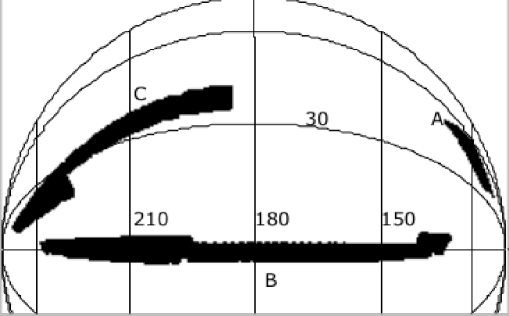
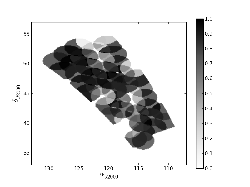
Figure 3.— (Top) The sky coverage of the galaxies used in this analysis, in orthographic projection centered on $\alpha_{J2000}=180^{\circ}$ and $\delta_{J2000}=0^{\circ}$. The regions A, B and C described in the text are marked. (Bottom) A zoom in of region A with the greyscale showing completeness. This region is the most contiguous of the three, and region B is the least contiguous owing to hardware problems in the early part of the year.

The clustering measurements in this paper are based on the data taken by BOSS up to end of July 2010, which includes 120,000 galaxies over 1,600 deg² of sky. However, the data prior to January 2010 were taken in commissioning mode and little of those data are of survey quality. Once we trim the data to contiguous regions (Fig. 3) with high redshift completeness and select galaxies at $z\sim 0.5$ we are left with $44,000$ galaxies, covering $580$ square degrees, which we have used in our analysis.

The sky coverage of our sample can be seen in Figure 3. We view the data as comprising three regions of the sky, hereafter referred to as A, B and C (see Figure). Galaxies in these regions are separated from those in any other region by several hundred Mpc, and we shall consider them independent. Convenient “rectangular” boundaries to the regions are

$$A : 105^{\circ}<\alpha_{J2000}<135^{\circ}\quad,\quad 25^{\circ}<\delta_{J2000}<60^{\circ}$$ (2)

$$B : 125^{\circ}<\alpha_{J2000}<240^{\circ}\quad,\quad-5^{\circ}<\delta_{J2000}<5^{\circ}$$ (3)

$$C : 185^{\circ}<\alpha_{J2000}<255^{\circ}\quad,\quad 10^{\circ}<\delta_{J2000}<45^{\circ}\quad.$$ (4)

These boundaries yield widths (heights) of 600 (700), 2600 (270) and 1600 (800) $h^{-1}$Mpc respectively at $z\simeq 0.5$. As we shall discuss below, the data are consistent with having the same clustering and redshift distribution in all three regions.

3. Clustering measures

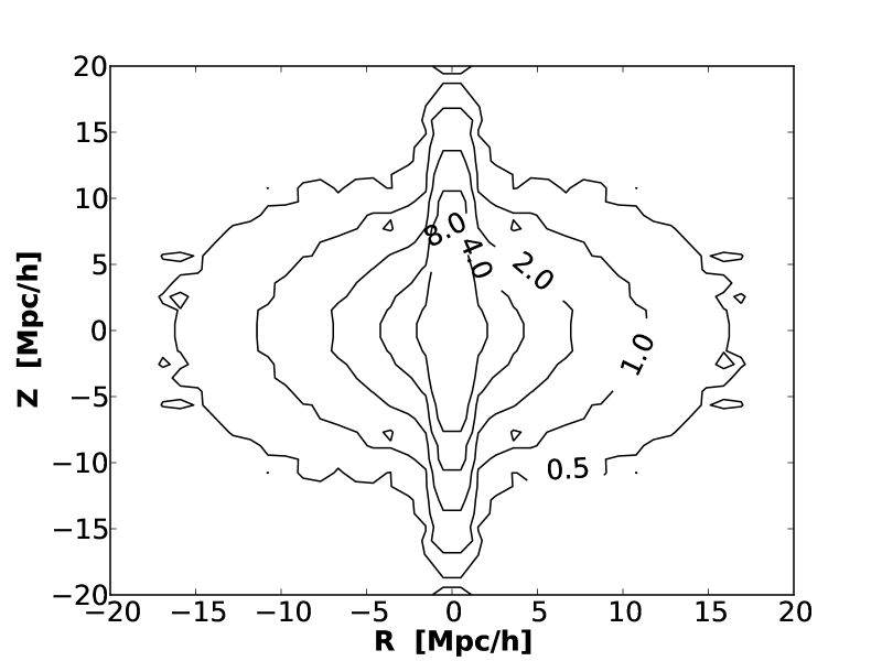
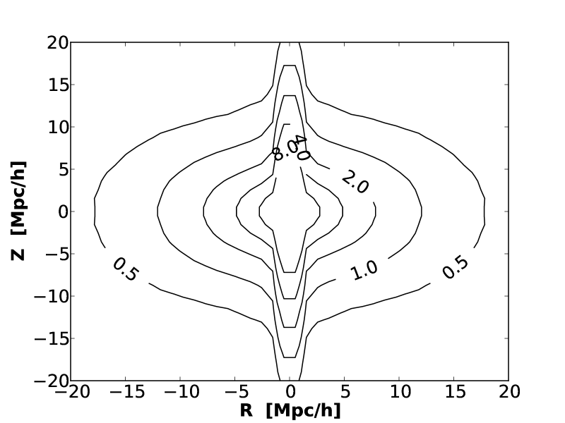
Figure 4.— Contours of the redshift-space correlation function, $\xi(R,Z)$, for our $0.4<z<0.7$ galaxy sample (see text). Note the characteristic elongation in the $Z$ direction at small $R$ (fingers-of-god) and squashing at large $R$ (super-cluster infall). The upper panel shows the results from the BOSS data, while the lower panel is from our mock catalogs. The level of agreement is quite good, as can be seen more quantitatively in later figures.

We compute several two-point, configuration-space clustering statistics in this paper. The basis for all of these calculations is the two-point galaxy correlation function on a two-dimensional grid of pair separations parallel and perpendicular to the line-of-sight: $\xi(R,Z)$.

To estimate the counts expected for unclustered objects while accounting for the complex survey geometry, we generate random catalogs with the detailed radial and angular selection functions of the sample but with $50\times$ the number of points. Numerous tests have confirmed that the survey selection function factorizes into an angular and a redshift piece. The redshift selection function can be taken into account by distributing the randoms according to the observed redshift distribution of the sample. The completeness on the sky is determined from the fraction of target galaxies in a sector for which we obtained a high-quality redshift, with the sectors being areas of the sky covered by a unique set of spectroscopic tiles (see Blanton et al., 2003; Tegmark et al., 2004). We use the Mangle software (Swanson et al., 2008) to track the angular completeness. In computing the redshift completeness we omit galaxies for which a redshift was already known from an earlier survey from both the target and success lists, and then later randomly sample such galaxies with the resulting completeness in constructing the input catalog. Since very few of our targets at $z\sim 0.5$ have existing redshifts this is a very small correction. Not all of the spectra taken resulted in a reliable redshift, and the failure probability has angular structure due to hardware limitations. These result in spatial signal-to-noise fluctuations in observations. We find no evidence that this failure is redshift dependent - low and high redshift failure regions have the same redshift distribution. We therefore apply a small angular correction for this spatial structure by up-weighting galaxies based on the signal-to-noise of each spectrum, and the probability of redshift measurement. This is a small correction and only affects our results at the percent level. To avoid issues arising from small-number statistics we only keep sectors with area larger than $10^{-4}\,$sr, or approximately $0.3$ sq. deg. At the observed mean density ($150\,{\rm deg}^{-2}$) we expect several tens of galaxies in any such region, enabling us to reliably determine the redshift completeness. We trim the final area to all sectors with completeness greater than 75%, producing our final sample of 44,000 galaxies, distributed as 5,000 in region A, 14,000 in region B and 24,000 in region C. After the cut the median, galaxy-weighted completeness is 88%, 84% and 88% in regions A, B and C respectively.

We estimate $\xi(R,Z)$ using the Landy & Szalay (1993) estimator

$$\xi(R,Z)=\frac{DD-2DR+RR}{RR}$$ (5)

where $DD$, $DR$ and $RR$ are suitably normalized numbers of (weighted) data-data, data-random and random-random pairs in bins of $(R,Z)$. We experimented with two sets of weights, one to correct for fiber collisions (described below) and one to reduce the variance of the estimator. The latter was

$$w_{i}=\frac{1}{1+\bar{n}(z_{i})\bar{\xi}_{V}(s)}$$ (6)

where $\bar{n}(z_{i})$ is the mean density at redshift $z_{i}$ and $\bar{\xi}_{V}$ is a model for the volume-integrated redshift-space correlation function within $s$. We approximated $\bar{\xi}_{V}=4\pi s_{0}^{2}s$, corresponding to $\xi(s)=(s/s_{0})^{-2}$ and took $s_{0}=8\,h^{-1}$Mpc. The details of the weighting scheme did not affect our final result on the scales of interest to us here – in fact dropping this weight altogether gave comparable results and so we neglect this weight in what follows.

We are unable to obtain redshifts for approximately 7% of the galaxies due to fiber collisions – no two fibers on any given observation can be placed closer than $62^{\prime\prime}$. At $z\simeq 0.5$ the $62^{\prime\prime}$ exclusion corresponds to $0.4\,h^{-1}$Mpc. Where possible we obtain redshifts for the collided galaxies in regions where plates overlap, but the remaining exclusion must be account for. We correct for the impact of this by (a) restricting our analysis to relatively large scales and (b) up-weighting galaxy-galaxy pairs in the analysis with angular separations smaller than $62^{\prime\prime}$. The weight is derived by comparing the angular correlation function of the entire photometric sample with that of the galaxies for which we obtained redshifts (Hawkins et al., 2003; Li et al., 2006; Ross et al., 2007). This ratio is very close to unity above $62^{\prime\prime}$ but significantly depressed below this scale. Note that in our situation there is a close correspondence between angular separation and transverse separation since our survey volume is a relatively narrow shell with reasonably large radius, so the number of pairs for which this correction is appreciable is quite small.

Contours of the 2D correlation function for our $0.4<z<0.7$ galaxy sample are shown in Figure 4. Note the characteristic elongation in the $Z$ direction at small $R$ (fingers-of-god) and squashing at large $R$ (super-cluster infall).

To mitigate the effects of redshift space distortions we follow standard practice and compute from $\xi(R,Z)$ the projected correlation function (e.g. Davis & Peebles, 1983)

$$w_{p}(R)=2\int_{0}^{\infty}dZ\ \xi(R,Z)\qquad.$$ (7)

In practice we integrate to $100\,h^{-1}$Mpc, which is sufficiently large to include almost all correlated pairs. We also compute the angularly averaged, redshift space correlation function, $\xi(s)$, and the cross-correlation between the CMASS sample selected from the imaging and the spectroscopic samples, $w_{\times}$. For all of these measures the full covariance matrix is computed from a set of mock catalogs based on a halo-occupation distribution (HOD) modeling of the data (§4 and Appendix A).

We now discuss each of the clustering measurements in turn, beginning with the real-space clustering.

3.1. Real-space clustering

$R$	0.40	0.71	1.27	2.25	4.00	7.11	12.65	22.50
$Rw_{p}$	167.68	134.49	147.63	168.29	208.77	242.70	255.89	230.36
$\sigma$	15.91	6.26	6.54	7.87	9.89	14.16	20.49	28.77
0.40	1.000	0.266	0.185	0.216	0.202	0.174	0.139	0.168
0.71	–	1.000	0.346	0.329	0.312	0.299	0.238	0.202
1.27	–	–	1.000	0.580	0.533	0.561	0.487	0.371
2.25	–	–	–	1.000	0.695	0.652	0.552	0.417
4.00	–	–	–	–	1.000	0.793	0.703	0.522
7.11	–	–	–	–	–	1.000	0.826	0.646
12.65	–	–	–	–	–	–	1.000	0.802
22.50	–	–	–	–	–	–	–	1.000

Table 1The projected correlation function data and covariance matrix, for 8 equally spaced bins in $\ln R$. Both $R$ and $w_{p}$ are measured in units of $h^{-1}$Mpc, with $R$ quoted at the bin mid-point. To reduce the condition number of the covariance matrix we quote means, errors and covariances on $Rw_{p}$, which removes much of the run of $w_{p}$ with scale and makes the quoted data points more similar in magnitude. The error bars, $\sigma_{i}$, from the diagonal of $C$, are broken out separately in the $3^{\rm rd}$ row and the correlation matrix, $C_{ij}/(\sigma_{i}\sigma_{j})$ is quoted in the lower part of the table. The full covariance matrix should be used in any fit, and the finite width of the $R$ bins should be included in theoretical predictions.

Figure 5.— The projected correlation function for the $0.4<z<0.7$ sample in regions A, B and C (lines) and for the combined sample (points with errors). The errors on the individual samples have been suppressed for clarity. The data are combined using the full covariance matrix, but only the diagonal elements are plotted. The $w_{p}$ implied by a power-law correlation function of slope $-1.8$ and correlation length of $7.5\,h^{-1}$Mpc forms a reasonable fit to the data with $1<R_{p}<10\,h^{-1}$Mpc but we do not plot it here for clarity. The (thick) long-dashed-dotted line shows the prediction of the best-fitting HOD model (§4), which provides a reasonable fit on all scales plotted (recall the errors are correlated).

The projected correlation function for the $0.4<z<0.7$ sample is shown in Figure 5. We chose 8 bins, equally spaced in $\ln R$ between $0.3\,h^{-1}$Mpc and $30\,h^{-1}$Mpc as a compromise between retaining the relevant information and generating stable covariance matrices via Monte-Carlo. The finite width of these bins should be borne in mind when comparing theoretical models to these data. The integration over $Z$ in Eq. (7) was done by Riemann sum using 100 linearly spaced bins in $Z$. The results were well converged at this spacing, because of the “smearing” of the correlation function along the line-of-sight due to redshift space effects. The data were analyzed separately in each of regions A, B and C and then combined in a minimum variance manner:

$$C^{-1}\mathbf{w}_{p}^{\rm(tot)}=\sum_{\alpha=A,B,C}\left[C^{(\alpha)}\right]^{-1}\mathbf{w}_{p}^{(\alpha)}$$ (8)

with

$$C^{-1}=\sum_{\alpha}\left[C^{(\alpha)}\right]^{-1}$$ (9)

where $\mathbf{w}_{p}^{(\alpha)}$ represents the vector of $w_{p}$ measurements from region $\alpha=$A, B or C. Not surprisingly, the combined result is dominated by the results from region C. To reduce the condition number of the covariance matrix, and the dynamic range in $w_{p}$, we fit throughout to $R\,w_{p}$ and quote the results in that form. The $w_{p}$ points are quite covariant, in part because the integration in Eq. (7) introduces a large mixing of power at different $R$, thus use of the full covariance matrix is essential. The error bars on the individual $\mathbf{w}_{p}^{(\alpha)}$ have been suppressed in the figure for clarity, and the square-root of the diagonal elements of the covariance matrix are shown as error bars on the combined result.

Figure 6.— The projected correlation function of the high- and low-$z$ samples (lines), split at the mid-point of the range, and of the full sample (points with errors), indicating that the clustering is evolving little and the sample can be analyzed in one wide redshift bin.

We also subdivided the redshift range into a low-$z$ and high-$z$ half, splitting at $z=0.55$, and found no statistically significant difference between the two samples (Figure 6; in the split samples the fiber collision correction is more uncertain, so the disagreement at the smallest $R$ point is not very significant). This result motivates our decision to analyze the data in a single redshift slice. Slow evolution of the clustering is expected for a highly biased population such as our luminous galaxies where the evolution of the bias approximately cancels the evolution of the dark matter clustering (Fry, 1996).

Even with only the 8 data points in $w_{p}$, deviations from a pure power-law correlation function are apparent. These can be traced to the non-power-law nature of the mass correlation function and the way in which the galaxies occupy dark matter halos – we will return to these issues in §4.

The calculation of errors in clustering measurements can be done in a number of different ways (see Norberg et al., 2009, for discussion). We first tried a bootstrap estimate, dividing the survey regions into 8-22, roughly equal area “pixels” and sampling from these regions with replacement (Efron & Gong, 1983). Unfortunately the irregular geometry and relatively small sky coverage meant we were not able to obtain a covariance matrix which was stable against changes in the pixelization. We anticipate that as the survey progresses this technique will become more robust. In the meantime, we computed the covariance from a series of mock catalogs derived from an iterative procedure using N-body simulations as described in Appendix A. We will show in Figure 13 that the distribution of $\chi^{2}$ from our mock catalogs encompasses the value obtained for the data in regions A, B and C if both are computed using the mock-based covariance matrix and the best-fitting HOD model (§4). This indicates that the measurements we obtain are completely consistent with being drawn from the underlying HOD model, given the finite number of galaxies and observing geometry.

3.2. Redshift-space clustering

The angle-averaged redshift space correlation function, $\xi(s)$, for the $0.4<z<0.7$ sample is shown in Figure 7. Again, the data were analyzed separately in each of regions A, B and C. The dot-dashed line shows the same power-law correlation function as described in Figure 5, while the solid line shows the predicted $\xi(s)$ from the model that best fits the $w_{p}$ data (above). The enhancement of clustering over the real-space result on large scales (Kaiser 1987, for a review see Hamilton 1998 and for recent developments see Pápai & Szapudi 2008; Shaw & Lewis 2008) is evident in the comparison of the data to the power-law. The good agreement between the data and the HOD-model below a few Mpc is indication that the satellite fraction in the model is close to that in the data and the relative motions of the satellite galaxies are close to the motions of the dark matter within the parent halos (i.e. any velocity bias is small). The characteristic down-turn on scales smaller than a few Mpc is expected from virial motions within halos and the motion of halos themselves. The excess power of the HOD model compared to the data on scales of a few Mpc can be mitigated by increasing the degrees of freedom in the model, for example by dropping the assumption that central galaxies move with the mean halo velocity or follow the dark matter radial profile or allowing a modest amount of satellite velocity bias.

On scales below tens of Mpc the violations of the distant observer approximation are small, but on larger scales they begin to become appreciable (Pápai & Szapudi, 2008) and should be included in any comparison between these data and a theoretical model (most noticeably for the higher multipoles).

Figure 7.— The redshift-space, isotropic correlation function for the $0.4<z<0.7$ sample in regions A, B and C (points). The same power-law correlation function which fits the $w_{p}$ data on intermediate scales, with $s_{0}=7.5\,h^{-1}$Mpc, is shown as the dot-dashed line while the solid line is the prediction for $\xi(s)$ from the best-fitting HOD model to $w_{p}$, assuming no velocity bias for satellites and that central galaxies are at rest in their halos. The good agreement below a few Mpc is an indication that the satellite fraction in the model is close to that in the data and any velocity bias is small.

3.3. Cross-correlation

Finally we consider $w_{p}$ computed from the cross-correlation of the imaging catalog with the spectroscopy – this allows us to isolate the galaxies to a narrow redshift shell and convert angles to (transverse) distances while at the same time being insensitive to the details of the spectroscopic selection including the issue of fiber collisions. As described in Padmanabhan et al. (2009), the angular cross correlation of the imaging and spectroscopic samples, with angles converted to distances using the redshift of the spectroscopic member, can be written as

$$w_{\times}(R)=\left\langle f(\chi)\right\rangle\ w_{p}(R)$$ (10)

where $f(\chi)$ is the normalized radial distribution of the photometric sample as a function of comoving distance, $\chi$, and the average is over the redshift distribution of the spectroscopic sample. Note that $w_{\times}(R)$ is dimensionless, with $f(\chi)$ having dimensions of inverse length and $w_{p}$ having dimensions of length.

Figure 8 shows the cross-correlation for regions A, B and C along with a power-law correlation function. The normalization of this figure differs from that of Figure 5 by a factor of $\langle f(\chi)\rangle\sim\mathcal{O}(10^{-3})$. Because the signal is suppressed by the width of $f(\chi)$ the estimate of $w_{p}$ from the cross-correlation is significantly noisier than that from the auto-correlation (see Myers et al., 2009, §2.1, for related discussion). The cross-correlation estimate is consistent with our auto-correlation results but we have not attempted to fit any models to it directly. We have extended the cross-correlation to smaller scales in the Figure to emphasize that there is significant power even on very small scales, which are difficult to probe directly with the auto-correlation function due to the fiber collision problem.

Figure 8.— The cross-correlation function, $w_{\times}(R)$, of the spectroscopic and photometric samples which is proportional to $w_{p}(R)$ (Eq. 10). The dot-dashed line represents a power-law correlation function. Error bars have been suppressed to avoid obscuring the figure. Due to the small value of $\langle f(\chi)\rangle\sim\mathcal{O}(10^{-3})$ the error bars are significant, especially at large scales, and are roughly the difference between the plotted lines for regions A, B and C.

4. Halo occupation modeling

In order to relate the observed clustering of galaxies with the clustering of the underlying mass, and to make realistic mock catalogs, we interpret our measurements within the context of the halo occupation distribution (Peacock & Smith, 2000; Seljak, 2000; Benson et al., 2000; White et al., 2001; Berlind & Weinberg, 2002; Cooray & Sheth, 2002). The halo occupation distribution describes the number and distribution of galaxies within dark matter halos. Since the clustering and space density of the latter are predictable functions of redshift, any HOD model makes predictions for a wide range of observational statistics. Rather than perform a simultaneous fit to the real- and redshift-space correlation functions (including their covariances) we choose to fit to the the real-space clustering only and show that the models which best fit these data also provide a reasonable description of the redshift-space clustering results. This avoids the need to make additional assumptions for modeling the redshift space correlation function. We also implicitly assume that we are measuring a uniform sample of galaxies across the entire redshift range, so that a single HOD makes sense. We tested this assumption by splitting the sample into high- and low-redshift subsamples.

We use a halo model which distinguishes between central and satellite galaxies with the mean occupancy of halos:

$$N(M)\equiv\left\langle N_{\rm gal}(M_{\rm halo})\right\rangle=N_{\rm cen}(M)+N_{\rm sat}(M)\quad.$$ (11)

Each halo either hosts a central galaxy or does not, while the number of satellites is Poisson distributed with a mean $N_{\rm sat}$. The mean number of central galaxies per halo is modeled with

$$N_{\rm cen}(M)=\frac{1}{2}\ {\rm erfc}\left[\frac{\ln(M_{\rm cut}/M)}{\sqrt{2}\sigma}\right]$$ (12)

and

$$N_{\rm sat}(M)=N_{\rm cen}\left(\frac{M-\kappa M_{\rm cut}}{M_{1}}\right)^{\alpha}$$ (13)

for $M>\kappa M_{\rm cut}$ and zero otherwise. This form implicitly assumes that halos do not host satellite galaxies without hosting centrals, which is at best an approximation, but this is reasonable for the purposes of computing projected clustering. Different functional forms have been proposed in the literature, but the current form is flexible enough for our purposes.

To explore the plausible range of HOD parameter space we applied the Markov Chain Monte Carlo method (MCMC; e.g., see Gilks et al., 1996) to the $w_{p}$ data using a $\chi^{2}$-based likelihood. This method generates a “chain” of HOD parameters whose frequency of appearance traces the likelihood of that model fitting the data. It works by generating random HODs from a trial distribution (in our case a multi-dimensional Gaussian), populating a simulation cube with galaxies according to that HOD, computing $w_{p}$ from the periodic box by pair counts and accepting or rejecting the HOD based on the relative likelihood of the fit. The step sizes and directions are determined from the covariance matrix of a previous run of the chain. Given the chain, the probability distribution of any statistic derivable from the parameters can easily be computed: we show the mean occupancy of halos as a function of mass, $N(M)$, in Figure 9, where the band indicates the $\pm 1\,\sigma$ spread within the chain. The mean (galaxy-weighted) halo mass is $\langle M_{180b}\rangle_{\rm gal}=(2.8\pm 0.15)\times 10^{13}\,h^{-1}M_{\odot}$ (we quote here the mass interior to a sphere within which the mean density is $180\times$ the background density for halo mass, rather than the friends-of-friends mass, to facilitate comparison with other work); while the satellite fraction is $(10\pm 2)\%$. The values of the HOD parameters are given in Table 2.

In addition to the purely statistical errors, shown in the figure and quoted above, there are systematic uncertainties. Our correction for fiber collisions only significantly impacts the smallest $R$ point in our calculation. If we increase the error on that point by a factor of 10, effectively removing it from the fit, the results change to $\langle M_{180b}\rangle_{\rm gal}=(2.6\pm 0.15)\times 10^{13}\,h^{-1}M_{\odot}$ and $(7\pm 2)\%$ respectively which are shifts of approximately $1\,\sigma$. Additional uncertainty arises from the uncertainty in the background cosmology (held fixed in this paper) and from methodological choices. A comparison of different methods for performing the halo modeling (using different mass definitions or halo profiles, analytic vs. numerical methods, different ways of enforcing halo exclusion, etc.) suggests an additional $\mathcal{O}(10\%)$ “systematic” uncertainty. It would be interesting to check the assumptions going into this HOD analysis, and the inferences so derived, with additional data and a luminosity dependent modeling.

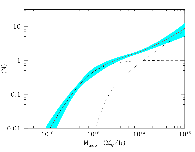
Figure 9.— The mean occupancy of halos as a function of halo mass for our full sample. The shaded band indicates the $\pm 1\,\sigma$ range determined from our Markov chain analysis. The dashed and dotted lines show the average $N_{\rm cen}$ and $N_{\rm sat}$, respectively.

The halo occupancy of massive galaxies at these redshifts has been investigated before based on both photometric (White et al., 2007; Blake et al., 2008; Brown et al., 2008; Padmanabhan et al., 2009) and spectroscopic (Ross et al., 2007, 2008; Wake et al., 2008; Zheng et al., 2009; Reid & Spergel, 2009) samples. Accounting for differences in sample selection and redshift range, our results appear quite consistent with the previous literature (see Fig. 10).

lg$M_{\rm cut}$	$13.08\pm 0.12$	($13.04$)
lg$M_{1}$	$14.06\pm 0.10$	($14.05$)
$\sigma$	$0.98\pm 0.24$	($0.94$)
$\kappa$	$1.13\pm 0.38$	($0.93$)
$\alpha$	$0.90\pm 0.19$	($0.97$)

Table 2The mean and standard deviation of the HOD parameters (see Eqs. 12 and 13) from our Markov chain. The particular values for our best-fit model are given in parentheses.

Figure 10.— The HOD parameters, $M_{\rm cut}$ and $M_{1-{\rm sat}}$, as a function of number density for a variety of intermediate redshift, massive galaxy samples from the literature (c.f. Fig. 12 of Brown et al. 2008). Here $M_{1-{\rm sat}}$ is the halo mass which hosts, on average, one satellite which is easier to compare when different functional forms for $N(M)$ are in use. The data are taken from Phleps et al. (2006), Mandelbaum et al. (2006), Kulkarni et al. (2007), Blake et al. (2008), Brown et al. (2008), Padmanabhan et al. (2009), Wake et al. (2008), Zheng et al. (2009) and this work, as noted in the legend. Error bars on the individual points have been suppressed for clarity, but are typically 0.1 dex. The solid line in the lower panel shows the halo mass function at $z=0.55$ for comparison. The value of $M_{\rm cut}$ for a sample of only central galaxies with no scatter between observable and halo mass would follow this line.

Our galaxies populate a broad range of halo masses, with an approximate power-law dependence of the mean number of galaxies per halo with halo mass for massive halos and a broad roll-off at lower halo masses. The low mass behavior is driven by the amplitude of the large-scale clustering in combination with the relatively high number density of our sample and encodes information about the scaling of the central galaxy luminosity with halo mass and its distribution. We find that the halos with masses $(2-3)\times 10^{13}\,h^{-1}M_{\odot}$ contain on average one of our massive galaxies. At these redshifts such halos are quite highly biased (see below), corresponding to galaxy groups, and we expect $b(z)\propto 1/D(z)$, where $D(z)$ is the linear growth rate, leading to an approximately constant clustering amplitude with redshift.

The majority of our galaxies are central galaxies residing in $10^{13}\,h^{-1}M_{\odot}$ halos, but a non-negligible fraction are satellites which live primarily in halos $\sim 10$ times more massive. The width of this “plateau” ($M_{1}/M_{\rm cut}$) is smaller than that found for less luminous systems at lower redshift, though it continues the trends seen in Zheng et al. (2009) for plateau width and satellite fraction as a function of luminosity. This increase in the satellite fraction is driving the visibility of the fingers-of-god in the correlation function (Figure 4) and the small-scale upturn in $w_{p}$.

An alternative view of the halo occupation is presented in Figure 11, which shows the probability that a galaxy in our sample is hosted by a halo of mass $M$. Note the broad range of halo masses probed by our galaxies, and the low probability of finding one of our galaxies in very high mass halos – which is a consequence of the sparsity of such halos at this redshift.

Figure 11.— The probability per $\log_{10}M_{\rm halo}$ (upper) or cumulative probability (lower) that a galaxy in our sample is hosted by a halo of mass $M_{\rm halo}$. Note the broad range of halo masses probed by our galaxies, and the low probability of finding one of our galaxies in very high mass halos (due to the sparsity of such halos at this redshift).

Figure 12.— The scale-dependence of the bias, $b(r)\equiv[\xi_{\rm gal}(r)/\xi_{\rm dm}(r)]^{1/2}$, predicted from our best-fit halo model and N-body simulations. The feature at a few Mpc has been seen in other analyses and occurs at the transition between the 1- and 2-halo contributions (see text). Note that the bias asymptotes to a constant, $b\simeq 2$, on large scales.

The N-body simulations can also be used to infer the scale-dependence of the bias, $b(r)\equiv[\xi_{\rm gal}(r)/\xi_{\rm dm}(r)]^{1/2}$, for our best-fitting halo model. This is shown in Figure 12, where we see that above $10-20\,h^{-1}$Mpc the bias approaches a constant, $b\simeq 2$. For our cosmology the linear growth factor at $z=0.55$ is $0.762$ so $b\sigma_{8}(z=0.55)=1.3$ and this is assumed constant across our redshift range. This is very similar to the results obtained for photometric LRG samples at comparable redshifts (Blake et al., 2007; Ross et al., 2007; Padmanabhan et al., 2007, 2009; Blake et al., 2008). The rapid rise of $b(r)$ at very small scales is expected, since it is well known that these galaxies exhibit an almost power-law correlation function at small scales while the non-linear $\xi_{\rm dm}(r)$ is predicted to fall below a power-law at small $r$. (Most galaxy pairs on these scales are central-satellite pairs, whereas for the dark matter there is no such distinction so $\xi_{\rm dm}$ is the convolution of the halo radial profile with itself.) The feature in $b(r)$ at a few Mpc occurs at the transition between the 1- and 2-halo contributions, i.e. pairs of galaxies that lie within a single dark matter halo vs. those which lie in separate halos, while the rise at slightly larger scales comes from the scale-dependence of the halo bias. Note that the combination of the high clustering amplitude and number density makes this sample particularly powerful for probing large-scale structure at $z\simeq 0.5$.

Finally, using the best-fitting HOD model from the chain and a series of N-body simulations we generate mock catalogs as described in more detail in Appendix A. These are passed through the observational masks and cuts in order to mimic the observations and can be analyzed in the same manner to generate a set of mock measurements from which we compute covariance matrices and other statistical quantities. We match the redshift distribution of the sample to our constant-number-density simulation boxes by randomly subsampling the galaxies as a function of redshift (with a 100% sampling at the peak near $z\simeq 0.55$). This is consistent with our assumption, earlier, that the HOD describes a single population of objects and the $dN/dz$ reflects observational selection effects. We obtain similar HODs fitting to the thinner redshift slices which lends credence to this view.

5. Discussion

The Baryon Spectroscopic Oscillation Survey is in the process of taking spectra for 1.5 million luminous galaxies and 150,000 quasars to make a precision determination of the scale of baryon oscillations and to study the growth of structure and the evolution of massive galaxies. We have presented measurements of the clustering of 44,000 massive galaxies at $z\sim 0.5$ from the first semester of BOSS data, showing that BOSS is performing well and that the galaxies we are targeting have properties in line with expectations (Schlegel et al., 2009).

The CMASS sample at $z\simeq 0.5$ has a large-scale bias of $b\simeq 2$ (Fig. 12), and a number density several times higher than the earlier, spectroscopic LRG sample of Eisenstein et al. (2001), making it an ideal sample for studying large-scale structure. The majority of our CMASS galaxies are central galaxies residing in $10^{13}\,h^{-1}M_{\odot}$ halos, but a non-negligible fraction are satellites which live primarily in halos $\sim 10$ times more massive.

The data through July 2010 do not cover enough volume to robustly detect the acoustic peak in the correlation function in this sample, one of the science goals of BOSS. While no definitive detection is possible at present, the error bars are anticipated to shrink rapidly as we collect more redshifts; BOSS should be able to constrain the acoustic scale at $z\sim 0.5$ within the next year, with the constraints becoming increasingly tight as the survey progresses.

Appendix A N-body simulations and mock catalogs

We make use of several simulations in this paper. The main set is 20 different realizations of the $\Lambda$CDM family with $\Omega_{m}=0.274$, $\Omega_{\Lambda}=0.726$, $h=0.7$, $n=0.95$ and $\sigma_{8}=0.8$ (in agreement with a wide array of observations). Briefly, each simulation employs an updated version of the TreePM code described in White (2002) to evolve $1500^{3}$ equal mass ($7.6\times 10^{10}\,h^{-1}M_{\odot}$) particles in a periodic cube of side length $1500\,h^{-1}$Mpc with a Plummer equivalent smoothing of $36\,h^{-1}$kpc. The initial conditions were generated by displacing particles from a regular grid using second order Lagrangian perturbation theory at $z=75$ where the rms displacement is $10\%$ of the mean inter-particle spacing. This TreePM code has been compared to a number of other codes and shown to perform well for such simulations (Heitmann et al., 2008). Recently the code has been modified to use a hybrid MPI+OpenMP approach which is particularly efficient for modern clusters.

For each output we found dark matter halos using the Friends of Friends (FoF) algorithm (Davis et al., 1985) with a linking length of $0.168$ times the mean interparticle spacing. This partitions the particles into equivalence classes roughly bounded by isodensity contours of $100\times$ the mean density. The position of the most-bound particle, the center of mass velocity and a random subset of the member particles are stored for each halo and used as input into the halo occupation distribution modeling and mock catalogs. Throughout we use the sum of the masses of the particles linked by the FoF algorithm as our basic definition of halo mass, except when quoting $\langle M_{180b}\rangle_{\rm gal}$ in §4 where we use spherical over-density (SO) masses to facilitate comparison with other work. Note we do not run a SO finder to define new groups. We use the FoF halo catalog, only computing a different mass for each FoF halo. In order to compute these SO masses we grow spheres outwards from the most bound particle in each FoF halo, stopping when the mean density of the enclosed material (including both halo and non-halo particles) is $180\times$ the background density. The total enclosed mass we denote by $M_{180b}$.

Figure 13.— The distribution of $\chi^{2}$ for $w_{p}$ from our mock catalogs (histograms) and from the data (vertical dashed lines) in regions A, B and C. The $\chi^{2}$ is computed for the measured or mock $w_{p}$ compared to the best-fitting HOD model using the covariance matrix computed from the mocks. The measurements we obtain are completely consistent with being drawn from the underlying HOD model, given the finite number of galaxies and observing geometry.

All of the mock observational samples are assumed to be iso-redshift, and “static” outputs are used as input to the modeling. The assumption of non-evolving clustering over the relevant redshift range is theoretically expected for a highly biased population, and also borne out by our modeling (§4) and measurements (§3).

Once a set of HOD parameter values has been chosen, we populate each halo in a given simulation with mock “galaxies”. The HOD provides the probabilities that a halo will contain a central galaxy and the number of satellites. The central galaxy is placed at the position of the most bound particle in the halo, and we randomly draw dark matter particles to represent the satellites, assuming that the satellite galaxies trace the mass profile within halos. This approach has the advantage of retaining any alignments between the halo material, the filamentary large-scale structure and the velocity field.

Since the observational geometry is in some cases highly elongated (Fig. 3), we use volume remapping (Carlson & White, 2010) on the periodic cubes to encompass many realizations of the sample within each box. The mock galaxies are then observed in a way analogous to the actual sample, with the completeness mask and redshift cuts applied to generate several hundred “mock surveys”. (Overall we have $1500$ mock surveys, divided into $900$, $360$ and $240$ mock surveys of regions A, B and C respectively. However they are not all completely independent as we have only $\sim 100$ times as much volume in the simulations as in the largest region, C.) For technical reasons, and since it only affects the smallest scale $w_{p}$ point, we do not model fiber collisions. Instead we increase the errors for that point by the square root of the ratio of the pair counts in the photometric sample to that in the spectroscopic sample (i.e. the same correction applied to the data-data pairs in computing $\xi(R,Z)$). This correction is appropriate in the limit that the error is dominated by Poisson counting statistics.

The covariance matrices for the clustering statistics are obtained from the mocks, and the entire procedure (reconstructing the best-fit with the new covariance matrix, recomputing the mock catalogs and recomputing the clustering) is iterated until convergence. Given a reasonable starting HOD, the procedure converges within two or three steps.

Over the range of scales probed in this paper the correlation function is quite well constrained and we find the distribution of $w_{p}$ values in the mocks is well fit by a Gaussian at each $R$. This suggests we are able to use a Gaussian form for the likelihood, which is backed up by the distribution of $\chi^{2}$ values seen in Figure 13.

References

- Abazajian et al. (2004) Abazajian, K., et al. 2004, AJ, 128, 502
- Bell et al. (2004) Bell, E. F., et al. 2004, ApJ, 608, 752
- Benson et al. (2000) Benson, A. J., Cole, S., Frenk, C. S., Baugh, C. M., & Lacey, C. G. 2000, MNRAS, 311, 793
- Berlind & Weinberg (2002) Berlind, A. A., & Weinberg, D. H. 2002, ApJ, 575, 587
- Blake et al. (2007) Blake, C., Collister, A., Bridle, S., & Lahav, O. 2007, MNRAS, 374, 1527
- Blake et al. (2008) Blake, C., Collister, A., & Lahav, O. 2008, MNRAS, 385, 1257
- Blanton et al. (2003) Blanton, M. R., Lin, H., Lupton, R. H., Maley, F. M., Young, N., Zehavi, I., & Loveday, J. 2003, AJ, 125, 2276
- Brown et al. (2008) Brown, M. J. I., et al. 2008, ApJ, 682, 937
- Carlson & White (2010) Carlson, J., & White, M. 2010, ApJS, 190, 311
- Cooray & Sheth (2002) Cooray, A., & Sheth, R. 2002, Phys. Rep., 372, 1
- Davis et al. (1985) Davis, M., Efstathiou, G., Frenk, C. S., & White, S. D. M. 1985, ApJ, 292, 371
- Davis & Peebles (1983) Davis, M., & Peebles, P. J. E. 1983, ApJ, 267, 465
- Doi et al. (2010) Doi, M., et al. 2010, AJ, 139, 1628
- Efron & Gong (1983) Efron, B., & Gong, G. 1983, American Statistician, 37, 36
- Eisenstein et al. (2001) Eisenstein, D. J., et al. 2001, AJ, 122, 2267
- Faber et al. (2007) Faber, S. M., et al. 2007, ApJ, 665, 265
- Fry (1996) Fry, J. N. 1996, ApJ, 461, L65+
- Fukugita et al. (1996) Fukugita, M., Ichikawa, T., Gunn, J. E., Doi, M., Shimasaku, K., & Schneider, D. P. 1996, AJ, 111, 1748
- Gilks et al. (1996) Gilks, W. R., Richardson, S., & Spiegelhalter, D. J. 1996, Markov Chain Monte Carlo in Practice (London: Chapman and Hall, 1966)
- Gregory & Thompson (1978) Gregory, S. A., & Thompson, L. A. 1978, ApJ, 222, 784
- Gunn et al. (1998) Gunn, J. E., et al. 1998, AJ, 116, 3040
- Gunn et al. (2006) —. 2006, AJ, 131, 2332
- Hamilton (1998) Hamilton, A. J. S. 1998, in Astrophysics and Space Science Library, Vol. 231, The Evolving Universe, ed. D. Hamilton, 185–+
- Hawkins et al. (2003) Hawkins, E., et al. 2003, MNRAS, 346, 78
- Heitmann et al. (2008) Heitmann, K., et al. 2008, Computational Science and Discovery, 1, 015003
- Huchra et al. (1983) Huchra, J., Davis, M., Latham, D., & Tonry, J. 1983, ApJS, 52, 89
- Humason et al. (1956) Humason, M. L., Mayall, N. U., & Sandage, A. R. 1956, AJ, 61, 97
- Joeveer & Einasto (1978) Joeveer, M., & Einasto, J. 1978, in IAU Symposium, Vol. 79, Large Scale Structures in the Universe, ed. M. S. Longair & J. Einasto, 241–250
- Kaiser (1987) Kaiser, N. 1987, MNRAS, 227, 1
- Kulkarni et al. (2007) Kulkarni, G. V., Nichol, R. C., Sheth, R. K., Seo, H., Eisenstein, D. J., & Gray, A. 2007, MNRAS, 378, 1196
- Landy & Szalay (1993) Landy, S. D., & Szalay, A. S. 1993, ApJ, 412, 64
- Li et al. (2006) Li, C., Kauffmann, G., Jing, Y. P., White, S. D. M., Börner, G., & Cheng, F. Z. 2006, MNRAS, 368, 21
- Lupton et al. (2001) Lupton, R., Gunn, J. E., Ivezić, Z., Knapp, G. R., & Kent, S. 2001, in Astronomical Society of the Pacific Conference Series, Vol. 238, Astronomical Data Analysis Software and Systems X, ed. F. R. Harnden Jr., F. A. Primini, & H. E. Payne, 269–+
- Mandelbaum et al. (2006) Mandelbaum, R., Seljak, U., Kauffmann, G., Hirata, C. M., & Brinkmann, J. 2006, MNRAS, 368, 715
- Maraston et al. (2009) Maraston, C., Strömbäck, G., Thomas, D., Wake, D. A., & Nichol, R. C. 2009, MNRAS, 394, L107
- Myers et al. (2009) Myers, A. D., White, M., & Ball, N. M. 2009, MNRAS, 399, 2279
- Norberg et al. (2009) Norberg, P., Baugh, C. M., Gaztañaga, E., & Croton, D. J. 2009, MNRAS, 396, 19
- Padmanabhan et al. (2009) Padmanabhan, N., White, M., Norberg, P., & Porciani, C. 2009, MNRAS, 397, 1862
- Padmanabhan et al. (2007) Padmanabhan, N., et al. 2007, MNRAS, 378, 852
- Padmanabhan et al. (2008) —. 2008, ApJ, 674, 1217
- Pápai & Szapudi (2008) Pápai, P., & Szapudi, I. 2008, MNRAS, 389, 292
- Peacock & Smith (2000) Peacock, J. A., & Smith, R. E. 2000, MNRAS, 318, 1144
- Phleps et al. (2006) Phleps, S., Peacock, J. A., Meisenheimer, K., & Wolf, C. 2006, A&A, 457, 145
- Pier et al. (2003) Pier, J. R., Munn, J. A., Hindsley, R. B., Hennessy, G. S., Kent, S. M., Lupton, R. H., & Ivezić, Ž. 2003, AJ, 125, 1559
- Reid & Spergel (2009) Reid, B. A., & Spergel, D. N. 2009, ApJ, 698, 143
- Ross et al. (2008) Ross, N. P., Shanks, T., Cannon, R. D., Wake, D. A., Sharp, R. G., Croom, S. M., & Peacock, J. A. 2008, MNRAS, 387, 1323
- Ross et al. (2007) Ross, N. P., et al. 2007, MNRAS, 381, 573
- Schlegel et al. (2009) Schlegel, D., White, M., & Eisenstein, D. 2009, in ArXiv Astrophysics e-prints, Vol. 2010, astro2010: The Astronomy and Astrophysics Decadal Survey, 314–+
- Schlegel et al. (1998) Schlegel, D. J., Finkbeiner, D. P., & Davis, M. 1998, ApJ, 500, 525
- Seljak (2000) Seljak, U. 2000, MNRAS, 318, 203
- Shaw & Lewis (2008) Shaw, J. R., & Lewis, A. 2008, Phys. Rev. D, 78, 103512
- Smith et al. (2002) Smith, J. A., et al. 2002, AJ, 123, 2121
- Stoughton et al. (2002) Stoughton, C., et al. 2002, AJ, 123, 485
- Swanson et al. (2008) Swanson, M. E. C., Tegmark, M., Hamilton, A. J. S., & Hill, J. C. 2008, MNRAS, 387, 1391
- Tegmark et al. (2004) Tegmark, M., et al. 2004, ApJ, 606, 702
- Wake et al. (2008) Wake, D. A., et al. 2008, MNRAS, 387, 1045
- White (2002) White, M. 2002, ApJS, 143, 241
- White et al. (2001) White, M., Hernquist, L., & Springel, V. 2001, ApJ, 550, L129
- White et al. (2007) White, M., Zheng, Z., Brown, M. J. I., Dey, A., & Jannuzi, B. T. 2007, ApJ, 655, L69
- York et al. (2000) York, D. G., et al. 2000, AJ, 120, 1579
- Zheng et al. (2009) Zheng, Z., Zehavi, I., Eisenstein, D. J., Weinberg, D. H., & Jing, Y. P. 2009, ApJ, 707, 554
- Zheng et al. (2005) Zheng, Z., et al. 2005, ApJ, 633, 791