Genome-Wide Significance Levels and Weighted Hypothesis Testing

Abstract

Genetic investigations often involve the testing of vast numbers of related hypotheses simultaneously. To control the overall error rate, a substantial penalty is required, making it difficult to detect signals of moderate strength. To improve the power in this setting, a number of authors have considered using weighted $p$-values, with the motivation often based upon the scientific plausibility of the hypotheses. We review this literature, derive optimal weights and show that the power is remarkably robust to misspecification of these weights. We consider two methods for choosing weights in practice. The first, external weighting, is based on prior information. The second, estimated weighting, uses the data to choose weights.

and

1 Introduction

Testing for association between genetic variation and a complex disease typically requires scanning hundreds of thousands of genetic polymorphisms. In a multiple testing situation, such as a genome-wide association study (GWAS), the null hypothesis is rejected for any test that achieves a $p$-value less than a predetermined threshold (usually on the order of $10^{-8}$). Data from these investigations has renewed interest in the multiple testing problem. The introduction of the false discovery rate and a procedure to control it by Benjamini and Hochberg (1995) inspired hope that this would be an effective way to control error while increasing power (Storey and Tibshirani, 2003; Sabatti, Service and Freimer, 2003). To further bolster power, recent statistical methods have been proposed that up-weight and down-weight hypotheses, based on prior likelihood of association with the phenotype (Genovese, Roeder and Wasserman, 2006; Roeder et al., 2006; Roeder, Wasserman and Devlin, 2007; Wang, Li and Bucan, 2007). Such prior information is often available in practice.

Weighted procedures multiply the threshold by the weight $w$, for each test, raising the threshold when $w>1$ and lowering it if $w<1$. To control the overall rate of false positives, a budget must be imposed on the weighting scheme, so that the average weight is one. If the weights are informative, the procedure improves power substantially, but, if the weights are uninformative, the loss in power is usually small. Surprisingly, aside from this budget requirement, any set of nonnegative weights is valid (Genovese, Roeder and Wasserman, 2006). While desirable in some respects, this flexibility makes it difficult to select weights for a particular analysis.

The first such weighting scheme appears to be Holm (1979). Related ideas can be found in Benjamini and Hochberg (1997), Chen et al. (2000), Genovese, Roeder and Wasserman (2006), Kropf et al. (2004), Rosenthal and Rubin (1983), Schuster, Kropf and Roeder (2004), Westfall and Krishen (2001), Westfall, Kropf and Finos (2004), Blanchard and Roquain (2008) and Roquain and van de Wiel (2008), among others. Several of these approaches use data dependent weights and yet maintain familywise error control. There are, of course, other ways to improve power aside from weighting. Some notable recent approaches include Rubin, Dudoit and van der Laan (2006), Storey (2007), Donoho and Jin (2004), Signoravitch (2006), Westfall, Krishen and Young (1998), Westfall and Soper (2001), Efron (2007) and Sun and Cai (2007). Of these, our approach is closest to Rubin, Dudoit and van der Laan (2006).

In some cases, the optimal weights can be estimated from the data. An approach developed by Westfall, Kropf and Finos (2004) utilizes quadratic forms to construct such weights; however, this approach assumes the individual measurements are normally distributed. This approach is suited to applications such as microarray data for which the observations are approximately normally distributed. We are interested in applications such as tests for genetic association. In this setting the individual observations are discrete, but the test statistics are approximately normally distributed.

In general, $p$-value weighting raises several important questions. How much power can we gain if we guess well in the weight assignment? How much power can we lose if we guess poorly? In this paper we show that the optimal weights have a simple parametric form and we investigate various approaches for estimating these weights. We also show the power is very robust to misspecification of the weights. In particular, in Section 3 we show that (i) sparse weights (few large weights and minimum weight close to 1) lead to huge power gains for well specified weights, but minute power loss for poorly specified weights; and (ii) in the nonsparse case, under weak conditions, the worst case power for poorly specified weights is typically better than the power obtained using equal weights.

We consider two methods for choosing the weights: (i) external weights, where prior information (based on scientific knowledge or prior data) singles out specific hypotheses (Section 4) and (ii) estimated weights where the data are used to construct weights (Section 5). External weights are prone to bias, while estimated weights are prone to variability. The two robustness properties reduce concerns about bias and variance.

To motivate this work consider an example (Figure 1) of external weighting that arises in genetic epidemiology. To identify variants of genes that induce greater susceptability to disease, two types of studies (linkage and association) are often performed. Whole genome linkage analysis has been conducted for most major diseases. These data can be summarized by a linkage trace, a smooth stochastic process $\{Z(s){}\dvtx{}s\in[0,L]\}$ where each $s$ corresponds to a location on the genome. At points that correspond to a variant of a gene of interest, the mean of the process $\mu(s)=E(Z(s))$ is a large positive value; however, due to extensive spatial correlation in the process, $\mu(s)$ is also nonzero in the vicinity of the variant. Tests for association between genetic polymorphisms and disease status for each of many genetic markers across the genome are also of interest. Like linkage analysis, the association statistics $\{T_{j}{}\dvtx{}j=1,\ldots,m\}$ map to spatial locations $\{s_{j}{}\dvtx{}j=1,\ldots,m\}$ on the genome. The number of tests $m$ can be large, on the order of 1,000,000. Until recently, whole genome association analysis was prohibitively expensive, but technological advances have now made such studies feasible. Due to the multiple testing correction, it is difficult to achieve sufficient power to obtain definitive results in these studies. The linkage trace provides one obvious source of information from which the weights can be constructed; see Section 6 for further elaboration. Unlike linkage analysis, however, the spatial correlation in association tests is weak. For this reason, other choices such as genetic pathways could offer a more promising source for weights in the future.

2 Background

2.1 Multiple Testing

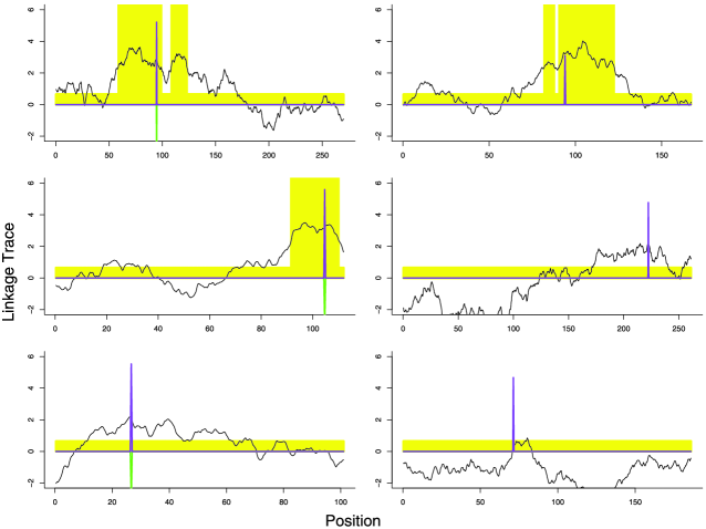
Figure 1: Linkage trace and weights for 6 chromosomes. The trace is the linkage statistic plotted as a function of position on the chromosome. The shading indicates which $p$-values were up/down weighted. The upspike is the association test statistic. The 3 downspikes indicate tests that were rejected using the binary weights.

Consider a multiple testing situation in which $m$ tests are being performed. Suppose $m_{0}$ of the null hypotheses are true and $m_{1}=m-m_{0}$ null hypotheses are false. We can categorize the $m$ tests as in Table 1. In this notation $F$ is the number of false positives. To control the familywise error rate, it is traditional to bound $P(F>0)$ at $\alpha$. When the tests are independent, the simplest way to control this probability is to reject only those tests for which the $p$-value is less than $\alpha/m$; this is called the Bonferroni procedure.

In 1995 Benjamini and Hochberg (BH) introduced a new approach to multiple hypothesis testing that controls the false discovery rate (FDR), defined as the expected fraction of false rejections among those hypotheses rejected. Let $P_{(1)}<\cdots<P_{(m)}$ be the ordered $p$-values from $m$ hypothesis tests, with $P_{(0)}\equiv 0$. Then, the BH procedure rejects any null hypothesis for which $P\leq T$ with

$$T=\max\biggl{\{}P_{(i)}{}\dvtx{}P_{(i)}\leq\frac{\alpha i}{m}\biggr{\}}.$$

This quantity is of more scientific relevance than the overall type I error rate in GWAS. Also, the procedure is more powerful than the Bonferroni method. Adaptive variants of the procedure can increase power further at little additional computational expense; see Benjamini, Krieger and Yekutieli (2006) andStorey (2002).

Table 1: $2\times 2$ classification of $m$ hypothesis tests

	$\bolds{H_{0}}$ rejected	$\bolds{H_{0}}$ not rejected	Total
$H_{0}$ true	$F$	$m_{0}-F$	$m_{0}$
$H_{0}$ false	$T$	$m_{1}-T$	$m_{1}$
Total	$S$	$m-S$	$m$

BH controls the false discovery rate at level $\alpha m_{0}/m$, where $m_{0}$ is the number of true null hypotheses. With certain dependence assumptions on the $p$-values, this is true regardless of how many nulls are true and regardless of the distribution of the $p$-values under the alternatives (Benjamini and Yekutieli, 2001; Blanchard and Roquain, 2009; Sarkar, 2002). Under some distributional assumptions, Genovese and Wasserman (2002) show that, asymptotically, the BH method corresponds to rejecting all $p$-values less than a particular $p$-value threshold $u^{*}$. Specifically, $u^{*}$ is the solution to the equation $H(u)=\beta u$ and $\beta=(\frac{1}{\alpha}-A_{0})/(1-A_{0})$, where $A_{0}=m_{0}/m$ and $H$ is the (common) distribution of the $p$-value under the alternative. The key result is that $\alpha/m\leq u^{*}\leq\alpha$, which shows that the BH method is intermediate between Bonferroni (corresponding to $\alpha/m$) and uncorrected testing (corresponding to $\alpha$). If $A_{0}$ is close to 0, however, as it usually is in GWA, then $\beta$ is a very large quantity and the power of the FDR is not much improved over the Bonferroni procedure.

The power of the BH method can be improved with adaptations. Blanchard and Roquain (2008) have given numerical comparisons of different adaptive procedures under dependence. Romano, Shaikh and Wolf (2008) have considered improving the adaptive procedure of Benjamini, Krieger and Yekutieli (2006) using the bootstrap. Sarkar and Heller (2008) have noted that the adaptive procedure of Benjamini et al. may not perform well compared to Storey’s (2002) procedure for certain parameter choices.

2.2 Weighted Multiple Testing

We are given hypotheses $H=(H_{1},\ldots,H_{m})$ and standardized test statistics $T=(T_{1},\ldots,T_{m})$, where $T_{j}\sim N(\xi_{j},1)$. Likewise, $T_{j}^{2}\sim\chi_{1}^{2}(\xi_{j}^{2})$. For a two-sided hypothesis, $H_{j}=1$ if $\xi_{j}\neq 0$ and $H_{j}=0$ otherwise. For the sake of parsimony, unless otherwise noted, results will be stated for a one-sided test where $H_{j}=1$ if $\xi_{j}>0$, although the results extend easily to the two-sided case. Let $\theta=(\xi_{1},\ldots,\xi_{m})$ denote the vector of means.

The $p$-values associated with the tests are $P=(P_{1},\ldots,P_{m})$, where $P_{j}=\overline{\Phi}(T_{j})$, $\overline{\Phi}=1-\Phi$ and $\Phi$ denotes the standard Normal cdf. Let $P_{(1)}\leq\cdots\leq P_{(m)}$ denote the sorted $p$-values and let $T_{(1)}\geq\cdots\geq T_{(m)}$ denote the sorted test statistics.

A rejection set $\mathcal{R}$ is a subset of $\{1,\ldots,m\}$. Say that $\mathcal{R}$ controls familywise error at level $\alpha$ if $\mathbb{P}(\mathcal{R}\cap\mathcal{H}_{0})\leq\alpha$, where $\mathcal{H}_{0}=\{j{}\dvtx{}H_{j}=0\}$. The Bonferroni rejection set is $\mathcal{R}=\{j{}\dvtx{}P_{j}<\alpha/m\}=\{j{}\dvtx{}T_{j}>z_{\alpha/m}\}$ where we use the notation $z_{\beta}=\overline{\Phi}^{-1}(\beta)$.

The weighted Bonferroni procedure (Rosenthal and Rubin, 1983; Genovese, Roeder and Wasserman, 2006) is as follows. Specify nonnegative weights $w=\break(w_{1},\ldots,w_{m})$ and reject hypothesis $H_{j}$ if

$$j\in\mathcal{R}=\biggl{\{}j{}\dvtx{}\frac{P_{j}}{w_{j}}\leq\frac{\alpha}{m}\biggr{\}}.$$ (1)

In the following lemma we show that as long as $m^{-1}\sum_{j}w_{j}\equiv\overline{w}=1$, the rejection set $\mathcal{R}$ controls familywise error at level $\alpha$. The second lemma includes a simple modification that will be needed later.

Lemma 2.1

If $\overline{w}=1$, then $\mathcal{R}$ controls familywise error at level $\alpha$.

Lemma 2.2

Suppose that $W_{j}=g(V_{j},c)$, $j=1,\break\ldots,m$, for some random variables $V_{1},\ldots,V_{m}$, some constant $c$ and some function $g$. Further, suppose that $V_{j}$ has a known distribution $H$ whenever $j\in\mathcal{H}_{0}$ and that $P_{j}$ is independent of $V_{j}$ for all $j\in\mathcal{H}_{0}$. The rule that rejects when $P_{j}\leq\alpha W_{j}/m$ controls familywise error at level $\alpha$ if $c$ is chosen to satisfy $\mathbb{E}_{H}(g(V_{j},c))\leq 1$.

Genovese, Roeder and Wasserman (2006) alsoshowed that false discovery methods benefit byweighting. Recall that the false discovery proportion (FDP) is

$${\rm FDP}=\frac{\mbox{number of false\ rejections}}{\mbox{number of rejections}}=\frac{|\mathcal{R}\cap\mathcal{H}_{0}|}{|\mathcal{R}|},$$

where the ratio is defined to be 0 if the denominator is 0. The false discovery rate (FDR) is $\mathrm{FDR}=\mathbb{E}({\rm FDP})$. Benjamini and Hochberg (1995) proved$\mathrm{FDR}\leq\alpha$ if $\mathcal{R}=\{j{}\dvtx{}P_{(j)}\leq T\}$ where $T=\break\max\{j{}\dvtx{}P_{(j)}\leq j\alpha/m\}$. Genovese, Roeder and Wasserman (2006) showed that $\mathrm{FDR}\leq\alpha$ if the $P_{j}$’s are replaced by $Q_{j}=P_{j}/w_{j}$ provided $\overline{w}=1$. This paper focuses on familywise error using the weighted procedure (1). Similar results hold for FDR and other familywise controlling procedures such as Holm’s test.

3 Power, Robustness and Optimality

The optimal weights, derived below, can be re-expressed as optimal cutoffs for testing. Specifically, rejecting when $P_{j}/w_{j}\leq\alpha/m$ is the same as rejection when $T_{j}>\xi_{j}/2+c/\xi_{j}$. This result can be obtained from Spjøtvoll (1972) and is identical to the result in Rubin, Dudoit and van der Laan (2006) obtained independently. The remainder of the paper, which shows some good properties of the weighted method, can thus also be considered as providing support for their method for selecting test specific cutoffs. In particular, Rubin et al. (2006)’s simulations indicate that even poorly specified estimates of the cutoffs $\xi_{j}/2+c/\xi_{j}$ can still perform well. In this section we provide insight into why this is true.

The power of a single, one-sided alternative in the unweighted case ($w_{j}=1$) is

$$\pi(\xi_{j},1)=\mathbb{P}(T_{j}>z_{\alpha/m})=\overline{\Phi}(z_{\alpha/m}-\xi_{j}).$$

The power in the weighted case is

$$\pi(\xi_{j},w_{j}) = \mathbb{P}\biggl{(}P_{j}<\frac{\alpha w_{j}}{m}\biggr{)}$$

$$= \mathbb{P}\biggl{(}T_{j}>\overline{\Phi}^{-1}\biggl{(}\frac{\alpha w_{j}}{m}\biggr{)}\biggr{)}$$

$$= \overline{\Phi}(z_{\alpha w_{j}/m}-\xi_{j}).$$

Weighting increases the power when $w_{j}>1$ and decreases the power when $w_{j}<1$ for the $j$th alternative.

Given $\theta=(\xi_{1},\ldots,\xi_{m})$ and $w=(w_{1},\ldots,w_{m})$, we define the average power

$$\frac{1}{m_{1}}\sum_{j=1}^{m}\pi(\xi_{j},w_{j})I(\xi_{j}>0),$$

where $m_{1}=\sum_{j=1}^{m}I(\xi_{j}>0)$. More generally, if $\xi$ is drawn from a distribution $Q$ and $w=w(\xi)$ is a weight function, we define the average power $\int\pi(\xi,\break w(\xi))I(\xi>0)\,dQ(\xi)/\int I(\xi>0)\,dQ(\xi)$. If we take $Q$ to be the empirical distribution of $(\xi_{1},\ldots,\xi_{m})$, then this reduces to the previous expression. In this formulation we require $w(\xi)\geq 0$ and $\int w(\xi)\,dQ(\xi)=1$.

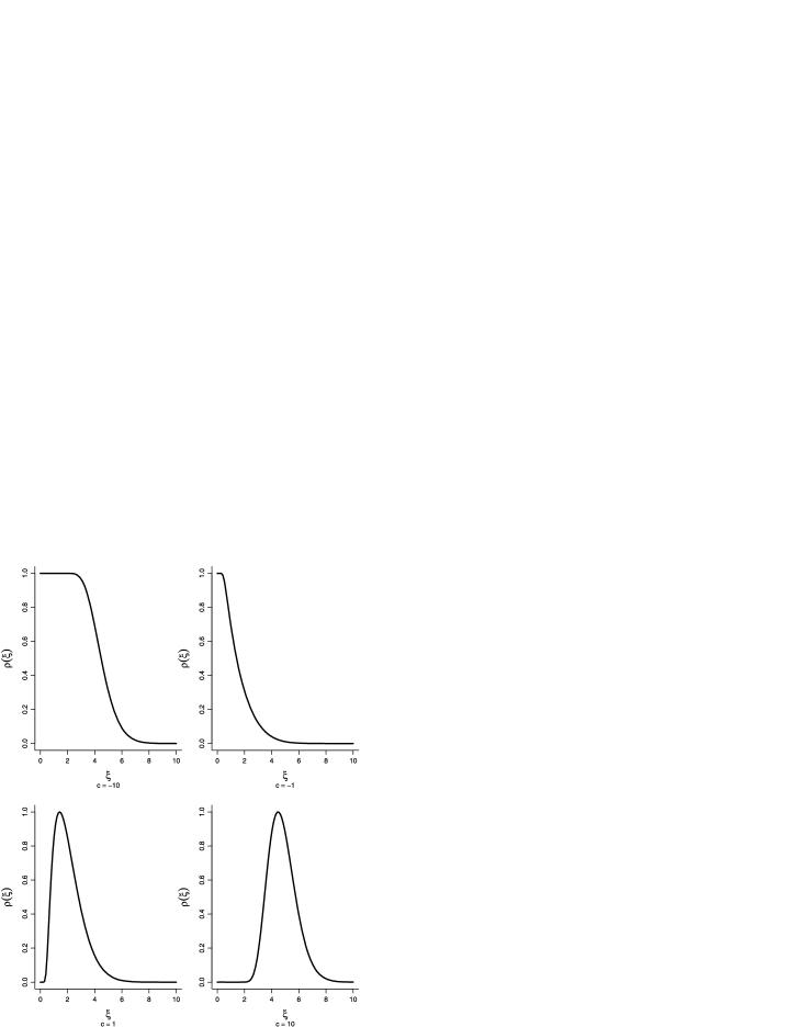
Figure 2: Optimal weight function $\rho_{c}(\xi)$ for various $c$. In each case $m=1000$ and $\alpha=0.05$. The functions are normalized to have maximum 1.

In the following theorem we see that the set of optimal weight functions form a one parameter family indexed by a constant $c$.

Theorem 3.1

Given $\theta=(\xi_{1},\ldots,\xi_{m})$, the optimal weight vector $w=(w_{1},\ldots,w_{m})$ that maximizes the average power subject to $w_{j}\geq 0$ and $\overline{w}=1$ is $w=(\rho_{c}(\xi_{1}),\ldots,\rho_{c}(\xi_{m}))$, where

$$\rho_{c}(\xi)=\biggl{(}\frac{m}{\alpha}\biggr{)}\overline{\Phi}\biggl{(}\frac{\xi}{2}+\frac{c}{\xi}\biggr{)}I(\xi>0),$$ (3)

and $c\equiv c(\theta)$ is defined by the condition

$$\frac{1}{m}\sum_{j=1}^{m}\rho_{c}(\xi_{j})=1.$$ (4)

The proof, essentially a special case of Spjøtvoll (1972), is in the Appendix. Figure 2 displays the function $\rho_{c}(\xi)$ for various values of $c$ (the function is normalized to have maximum 1 for easier visualization). The result generalizes to the case where the alternative means are random variables with distribution $Q$ in which case $c$ is defined by $\int\rho_{c}(\xi)\,dQ(\xi)=1$.

From (3) and (3) we have immediately:

Lemma 3.2

The power at an alternative with mean $\xi$ under optimal weights is $\overline{\Phi}(c/\xi-\xi/2)$. The average power under optimal weights, which we call the oracle power, is

$$\frac{1}{m_{1}}\sum_{j=1}^{m}\overline{\Phi}\biggl{(}\frac{c}{\xi_{j}}-\frac{\xi_{j}}{2}\biggr{)}I(\xi_{j}>0),$$

where $m_{1}=\sum_{j}I(\xi_{j}>0)$.

The oracle power is not attainable since the optimal weights depend on $\theta=(\xi_{1},\ldots,\xi_{m})$. In practice, the weights will either be chosen by prior information or by estimating the $\xi$’s. This raises the following question: how sensitive is the power to correct specification of the weights? Now we show that the power is very robust to weight misspecification.

Sparse weights (minimum weight close to 1) are highly robust. If most weights are less than 1 and the minimum weight is close to 1, then correct specification (large weights on alternatives) leads to large power gains but incorrect specification (large weights on nulls) leads to little power loss.

Worst case analysis. Weighted hypothesis testing, even with poorly chosen weights, typically does as well or better than Bonferroni except when the the alternative means are large, in which both have high power.

Let us now make these statements precise. Also, see Genovese, Roeder and Wasserman (2006) and Roeder et al. (2006) for other results on the effect of weight misspecification.

Property I. Consider first the case where the weights take two distinct values and the alternatives have a common mean $\xi$. Let $\varepsilon$ denote the fraction of hypotheses given the larger of the two values of the weights $B$. Then, the weight vector $w$ is proportional to

$$(\underbrace{B,\ldots,B}_{k\ \mathrm{terms}},\underbrace{1,\ldots,1}_{m-k\ \mathrm{terms}}),$$

where $k=\varepsilon m$ and $B>1,$ and, hence, the normalized weights are

$$w=(\underbrace{w_{1},\ldots,w_{1}}_{k\ \mathrm{terms}},\underbrace{w_{0},\ldots,w_{0}}_{m-k\ \mathrm{terms}}),$$

where

$$w_{1}=\frac{B}{\varepsilon B+(1-\varepsilon)},\quad w_{0}=\frac{1}{\varepsilon B+(1-\varepsilon)}.$$

We say that the weights are sparse if $\varepsilon$ is small. Provided $B$ is considerably less than $1/\varepsilon$, most weights are near 1 in the sparse case.

Rather than investigate the average power, we focus on a single alternative with mean $\xi$. The power gain by up-weighting this hypothesis is the power under weight $w_{1}$ minus the unweighted power$\pi(\xi,w_{1})-\pi(\xi,1)$. Similarly, the power loss for down-weighting is $\pi(\xi,1)-\pi(\xi,w_{0})$. The gain minus the loss, which we call the robustness function, is

$$R(B,\varepsilon) \equiv \bigl{(}\pi(\xi,w_{1})-\pi(\xi,1)\bigr{)}$$

$${}+\bigl{(}\pi(\xi,1)-\pi(\xi,w_{0})\bigr{)}$$

$$= \overline{\Phi}(z_{\alpha w_{1}/m}-\xi)+\overline{\Phi}(z_{\alpha w_{0}/m}-\xi)$$

$${}-2\overline{\Phi}(z_{\alpha/m}-\xi).$$

The gain outweighs the loss if and only if $R(B,\varepsilon)>0$ (Figure 3).

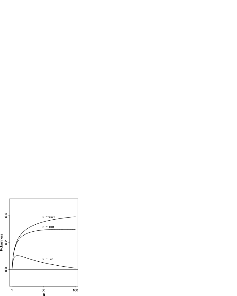
Figure 3: Robustness function for $m=1000$. In this example, $\xi=z_{\alpha/m}$ which has power 1$/$2 without weighting. The gain of correct weighting far outweighs the loss for incorrect weighting as long as the fraction of large weights $\varepsilon$ is small.

In the sparse weighting scenario $k$ is small and $w_{0}\approx 1$ by assumption, consequently, an analysis of $R(B,\varepsilon)$ sheds light on the effect of weighting on power, without the added complications involved in a full analysis of average power.

Theorem 3.3

Fix $B>1$. Then, $\lim_{\varepsilon\to 0}R(B,\break\varepsilon)>0$. Moreover, there exists $\varepsilon^{*}(B)>0$ such that $R(B,\varepsilon)>0$ for all $\varepsilon<\varepsilon^{*}(B)$.

We can generalize this beyond the two-valued case as follows. Let $w$ be any weight vector such that $\overline{w}=1$. Now define the (worst case) robustness function

$$R(\xi) \equiv \min_{\{j:w_{j}>1,H_{j}=1\}}\{\pi(\xi,w_{j})-\pi(\xi,1)\}$$

$${}-\max_{\{j:w_{j}<1,H_{j}=1\}}\{\pi(\xi,1)-\pi(\xi,w_{j})\}.$$

We will see that $R(\xi)>0$ under weak conditions and that the maximal robustness is obtained for $\xi$ near the Bonferroni cutoff $z_{\alpha/m}$.

Theorem 3.4

A necessary and sufficient condition for $R(\xi)>0$ is

$$R_{b,B}(\xi) \equiv {\Phi}(z_{\alpha B/m}-\xi)+{\Phi}(z_{\alpha b/m}-\xi)$$

$${}-2{\Phi}(z_{\alpha/m}-\xi)\leq 0,$$

where $B=\min\{w_{j}:w_{j}>1\}$, $b=\min\{w_{j}\}$. Moreover,

$$R_{b,B}(\xi)=-\Delta(\xi)+O(1-b),$$

where

$$\Delta(\xi)=\bigl{(}{\Phi}(z_{\alpha/m}-\xi)-{\Phi}(z_{\alpha B/m}-\xi)\bigr{)}>0$$

and, as $b\to 1$, $\mu(\{\xi\dvtx R(\xi)<0\})\to 0$ and$\inf_{\xi}R(\xi)\to 0$.

Based on the theorem, we see that there is overwhelming robustness as long as the minimum weight is near 1. Even in the extreme case $b=0$, there is still a safe zone, an interval of values of $\xi$ over which $R(\xi)>0$.

Lemma 3.5

Suppose that $B\geq 2$. Then there exists $\xi_{*}>0$ such that $R_{B,b}(\xi)>0$ for all $0\leq\xi\leq\xi_{*}$ and all $b$. An upper bound on $\xi_{*}$ is $z_{\alpha/m}-1/(z_{\alpha/m}-z_{B\alpha/m})$.

Property II. Even if the weights are not sparse, the power of the weighted test tends to be acceptable.

The result holds even though the weights themselves can be very sensitive to changes in $\theta$. Consider the following example. Suppose that $\theta=(\xi_{1},\ldots,\xi_{m})$ where each $\xi$ is equal to either 0 or some fixed number $\xi$. The empirical distribution of the $\xi_{j}$’s is thus $Q=(1-a)\delta_{0}+a\delta_{\xi}$, where $\delta$ denotes a point mass and $a$ is the fraction of nonzero means. The optimal weights are $0$ for $\xi_{j}=0$ and $1/a$ for $\xi_{j}=\xi$. Let $\tilde{Q}=(1-a-\gamma)\delta_{0}+\gamma\delta_{u}+a\delta_{\xi}$, where $u$ is a small positive number. Since we have only moved the mass at 0 to $u$, and $u$ is small, we would hope that $w(\xi)$ will not change much. But this is not the case. Set $\xi=A+\sqrt{A2-2c}$, $u=B-\sqrt{B2-2c}$, where

$$A = \overline{\Phi}^{-1}\biggl{(}\frac{\alpha}{(m(\gamma K+a))}\biggr{)},$$

$$B = \overline{\Phi}^{-1}\biggl{(}\frac{K\alpha}{(m(\gamma K+a))}\biggr{)}.$$

This arrangement yields weights $w_{0}$ and $w_{1}$ on $u$ and $\xi$ such that $w_{0}/w_{1}=K$. For example, if $m=1000$, $\alpha=0.05$, $a=0.1$, $\gamma=0.1$, $K=1000$ and $c=0.1$, then $u=0.03$ and $\xi=9.8$. The optimal weight on $\xi$ under $Q$ is 10 but under $\tilde{Q}$ it is $0.00999$ and so is reduced by a factor of 1001. More generally, we have the following result which shows that the weights are, in a certain sense, a discontinuous function of $\theta$.

Lemma 3.6

Fix $\alpha$ and $m$. For any $\delta>0$ and $\varepsilon>0$ there exists $Q=(1-a)\delta_{0}+a\delta_{\xi}$ and $\tilde{Q}=(1-a-\gamma)\delta_{0}+\gamma\delta_{u}+a\delta_{\xi}$ such that $d(Q,\tilde{Q})<\delta$, and$\tilde{\rho}(\xi)/\rho(\xi)<\varepsilon$, where $a=\alpha/4$, $d(Q,\tilde{Q})=\break\sup_{\xi}|Q(-\infty,\xi],\tilde{Q}(-\infty,\xi]|$ is the Kolmogorov–Smnirnov distance, $\rho$ is the optimal weight function for $Q$ and $\tilde{\rho}$ is the optimal weight function for $\tilde{Q}$.

Fortunately, this feature of the weight function does not pose a serious hurdle in practice because it is possible to have high power even with poor weights. In Figure 4 the plots on the left show the power as a function of the alternative mean $\xi$. The dark solid line shows the lowest possible power assuming the weights were estimated as poorly as possible (under conditions specified below). The lighter solid line is the power of the unweighted (Bonferroni) method. The dotted line shows the power under theoretically optimal weights. The worst case weighted power is typically close to or larger than the Bonferroni power except for large $\xi$ when they are both large.

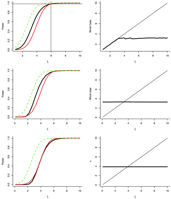
Figure 4: Power as a function of the alternative mean $\xi$. In these plots, $a=0.01$, $m=1000$ and $\alpha=0.05$. There are $(1-a)m$ nulls and $ma$ alternatives with mean $\xi$. The left plots show what happens when the weights are incorrectly computed assuming that a fraction $\gamma$ of nulls are actually alternatives with mean $u$. In the top plot, we restrict $0<u<\xi$. In the second and third plots, no restriction is placed on $u$. The top and middle plots have $\gamma=0.1,$ while the third plot has $\gamma=1-a$ (all nulls misspecified as alternatives). The dark solid line shows the lowest possible power assuming the weights were estimated as poorly as possible. The lighter solid line is the power of the unweighted (Bonferroni) method. The dotted line is the power under the optimal weights. The vertical line in the top plot is at $\xi_{*}$. The weighted method beats unweighted for all $\xi<\xi_{*}$. The right plot shows the least favorable $u$ as a function of $\xi$. That is, mistaking $\gamma m$ nulls for alternatives with mean $u$ leads to the worst power. Also shown is the line $u=\xi$.

To begin formal analysis, assume that each mean is either equal to $0$ or $\xi$ for some fixed $\xi>0$. Thus, the empirical distribution is $Q=(1-a)\delta_{0}+a\delta_{\xi}$, where $\delta$ denotes a point mass and $a$ is the fraction of nonzero $\xi_{j}$’s. The optimal weights are $1/a$ for hypotheses whose mean is $\xi$. To study the effect of misspecification error, consider the case where $\gamma m$ nulls are mistaken for alternatives with mean $u>0$. This corresponds to misspecifying $Q$ to be $\tilde{Q}=(1-a-\gamma)\delta_{0}+\gamma\delta_{u}+a\delta_{\xi}$. We will study the effect of varying $u$, so let $\pi(u)$ denote the power at the true alternative $\xi$ as a function of $u$. Also, let $\pi_{\rm Bonf}$ denote the power using equal weights (Bonferroni). Note that changing $Q=(1-a)\delta_{0}+a\delta_{\xi}$ to $Q=(1-a)\delta_{0}+a\delta_{\xi^{\prime}}$ for $\xi^{\prime}\neq\xi$ does not change the weights.

As the weights are a function of $c$, we first need to find $c$ as a function of $u$. The normalization condition (4) reduces to

$$\gamma\overline{\Phi}\biggl{(}\frac{u}{2}+\frac{c}{u}\biggr{)}+a\overline{\Phi}\biggl{(}\frac{\xi}{2}+\frac{c}{\xi}\biggr{)}=\frac{\alpha}{m},$$ (6)

which implicitly defines the function $c(u)$. First we consider what happens when $u$ is restricted to be less than $\xi$.

Theorem 3.7

Assume that $\alpha/m\leq\gamma+a\leq 1$. Let $Q=(1-a)\delta_{0}+a\delta_{\xi}$ and $\tilde{Q}=(1-a-\gamma)\delta_{0}+\gamma\delta_{u}+a\delta_{\xi}$ with $0\leq u\leq\xi$. Let $C(\xi)=\sup_{0\leq u\leq\xi}c(u)$ and define $\xi_{0}=z_{\alpha/(m(\gamma+a))}$:

1. For $\xi\leq\xi_{0}$, $C(\xi)=\xi\xi_{0}-\xi^{2}/2$. For $\xi>\xi_{0}$, $C(\xi)$ is the solution to

   $$\gamma\overline{\Phi}\bigl{(}\sqrt{2c}\bigr{)}+a\overline{\Phi}\biggl{(}\frac{c}{\xi}+\frac{\xi}{2}\biggr{)}=\frac{\alpha}{m}.$$

   In this case, $C(\xi)=z^{2}_{\alpha/(m\gamma)}/2+O(a)$.

2. Let $\xi_{*}=z_{\alpha/m}+\sqrt{z_{\alpha/m}^{2}-z_{q}^{2}}$, where $q=\alpha(1-a)/(m\gamma)$. For $\xi<\xi_{*}$,

   $$\inf_{0<u<\xi}\pi(u)\geq\pi_{\rm Bonf}.$$ (7)

   For $\xi\geq\xi_{*}$ we have

   $$\hskip 25.0pt\inf_{0<u<\xi}\pi(u) \geq \overline{\Phi}\biggl{(}\frac{z^{2}_{\alpha/(m\gamma)}-\xi_{*}^{2}}{2\xi_{*}}\biggr{)}-O(a)$$ (8)

   $$\approx 1-\overline{\Phi}\Biggl{(}\sqrt{2\log\frac{1-a}{\gamma}}\Biggr{)}-O(a)$$ (9)

   $$\geq 1-\frac{\gamma}{1-a}-O(a).$$ (10)

The factor $\overline{\Phi}(\sqrt{2\log(1-a)/\gamma})\approx\gamma/(1-a)$ is the worst case power deficit due to misspecification. Now we drop the assumption that $u\leq\xi$.

Theorem 3.8

Let $Q=(1-a)\delta_{0}+a\delta_{\xi}$ and let $Q_{u}\equiv(1-a-\gamma)\delta_{0}+\gamma\delta_{u}+a\delta_{\xi}$. Let $\pi_{u}$ denote the power at $\xi$ using the weights computed under $Q_{u}$.

1. The least favorable $u$ is $u_{*}\equiv\mathop{\arg\min}_{u\geq 0}\pi_{u}=\break\sqrt{2c_{*}}=z_{\alpha/(m\gamma)}+O(a)$, where $c_{*}$ solves

   $$\gamma\overline{\Phi}\bigl{(}\sqrt{2c_{*}}\bigr{)}+a\overline{\Phi}\biggl{(}\frac{\xi}{2}+\frac{c_{*}}{\xi}\biggr{)}=\frac{\alpha}{m}$$

   and $c_{*}=z^{2}_{\alpha/(m\gamma)}/2+O(a)$.

2. The minimal power is

   $$\inf_{u}\pi_{u}=\overline{\Phi}\biggl{(}\frac{c_{*}}{\xi}-\frac{\xi}{2}\biggr{)}=\overline{\Phi}\biggl{(}\frac{z_{\alpha/(m\gamma)}^{2}-\xi^{2}}{2\xi}\biggr{)}+O(a).$$

3. A sufficient condition for $\inf_{u}\pi_{u}$ to be larger than the power of the Bonferroni method is $\xi\geq z_{\alpha/m}+\sqrt{z^{2}_{\alpha/m}-z^{2}_{\alpha/(m\gamma)}}+O(a)$.

4 Choosing External Weights

Figure 5: Top plot: turnaround point $B_{0}(\varepsilon)$ versus $\varepsilon$. Bottom plot shows the robustness function $R(B,0.1)$ versus $B$. The turnaround point $B_{0}(\varepsilon)$ is shown with a vertical dotted line.

One approach to choosing external weights (or test statistic cutoffs) is to use empirical Bayes methods to model prior information while being careful to preserve error control as in Westfall and Soper (2001), for example. Here we consider a simplemethod that takes advantage of the robustness properties we have discussed. We will focus here on the two-valued case. Thus,

$$w=(\underbrace{w_{1},\ldots,w_{1}}_{k\ \mathrm{terms}},\underbrace{w_{0},\ldots,w_{0}}_{m-k\ \mathrm{terms}}),$$

where $k=\varepsilon m$, $w_{1}=B/(\varepsilon B+(1-\varepsilon))$ and $w_{0}=1/(\varepsilon B+(1-\varepsilon))$. In practice, we would typically have a fixed fraction of hypotheses $\varepsilon$ that we want to give more weight to. The question is how to choose $B$. We will focus on choosing $B$ to produce weights with good properties at interesting values of $\xi$. Now large values of $\xi$ already have high power. Very small values of $\xi$ have extremely low power and benefit little by weighting. This leads us to focus on constructing weights that are useful for a marginal effect, defined as the alternative $\xi_{0}$ that has power 1$/$2 when given weight 1. Thus, the marginal effect is $\xi_{0}=z_{\alpha/m}$. In the rest of this section then we assume that all nonzero $\xi_{j}$’s are equal to $\xi_{0}$. Of course, the validity of the procedure does not depend on this assumption being true.

Fix $0<\varepsilon<1$ and vary $B$. As we increase $B$, we will eventually reach a point $B_{0}(\varepsilon)$ where $R(B,\varepsilon)<0$, which we call the turnaround point. Formally, $B_{0}(\varepsilon)=\sup\{B{}\dvtx{}R(B,\varepsilon)>0\}$. The top panel in Figure 5 shows $B_{0}(\varepsilon)$ versus $\varepsilon$, which shows that for small $\varepsilon$ we can choose $B$ large without loss of power. The bottom panel shows $R(B,\varepsilon)$ for $\varepsilon=0.1$. Ideally, for a given $\varepsilon,$ one chooses $B$ near $B_{*}(\varepsilon)$, the value of $B$ that maximizes $R(B,\varepsilon)$.

Theorem 4.1

Fix $0<\varepsilon<1$. As a function of $B$, $R(B,\varepsilon)$ is unimodal and satisfies $R(1,\varepsilon)=1$, $R^{\prime}(1,\varepsilon)>0$ and $R(\infty,\varepsilon)<0$. Hence, $B_{0}(\varepsilon)$ exists and is unique. Also, $R(B,\varepsilon)$ has a unique maximum at some point $B^{*}(\varepsilon)$ and $R(B^{*}(\varepsilon),\varepsilon)>0$.

When $\varepsilon$ is very small, $B$ can be large, provided $w_{0}\approx 1$. For example, suppose we want to increase the chance of rejecting one particular hypothesis so that $\varepsilon=1/m$. Then,

$$w_{1}=\frac{mB}{B+m-1}\approx B,\quad w_{0}=\frac{1}{B+m-1}\approx 1$$

and

$$\lim_{m\to\infty}\lim_{B\to\infty}\pi(\xi_{j},w_{1})=1,$$

$$\eqntext{\displaystyle\mbox{while}\lim_{m\to\infty}\lim_{B\to\infty}\pi(\xi_{j},w_{0})=\frac{1}{2}.}$$ (11)

The next results show that binary weighting schemes are optimal in a certain sense. Suppose we want to have at least a fraction $\varepsilon$ with high power $1-\beta$ and otherwise we want to maximize the minimum power.

Theorem 4.2

Consider the following optimization problem: Given $0<\varepsilon<1$ and $0<\beta<1/2$, find a vector $w=(w_{1},\ldots,w_{m})$ that maximizes $\min_{j}\pi(\xi_{m},\break w_{j})$ subject $\overline{w}=1$, and $\#\{j{}\dvtx{}\pi(w_{j},\xi_{m})\geq 1-\beta\}/m\geq\varepsilon$. The solution is given by $c=\overline{\Phi}(z_{\alpha/m}+z_{1-\beta})$, $B=cm(1-\varepsilon)/(\alpha-\varepsilon cm)$, $w_{1}=B/(\varepsilon B+(1-\varepsilon))$, $w_{0}=1/(\varepsilon B+(1-\varepsilon))$ and $k=\varepsilon m$.

If our goal is to maximize the number of alternatives with high power while maintaining a minimum power loss, the solution is given as follows.

Theorem 4.3

Consider the following optimization problem: Given $0<\beta<1/2$, find a vector $w=(w_{1},\ldots,w_{m})$ that maximizes $\#\{j{}\dvtx{}\pi(w_{j},\xi_{m})\geq 1-\beta\}$ subject to $\overline{w}=1,\mbox{ and }\min_{j}\pi(w_{j},\xi_{m})\geq\delta$. The solution is

$$w_{1} = \frac{m}{\alpha}\overline{\Phi}(z_{\alpha/m}+z_{1-\beta}),\quad w_{0}=\frac{m}{\alpha}\overline{\Phi}(z_{\alpha/m}+z_{\delta}),$$

$$\varepsilon = \frac{1-w_{0}}{w_{1}-w_{0}}$$

and $k=m\varepsilon$.

A special case that falls under this theorem permits the minimum power to be 0. In this case $w_{0}=0$ and $\varepsilon=1/w_{1}$.

5 Estimated Weights

In practice, $\xi_{j}$ is not known, so it must be estimated to utilize the weight function. A natural choice is to build on the two stage experimental design (Satagopan and Elston, 2003; Wang et al., 2006) and split the data into subsets, using one subset to estimate $\xi_{i}$, and hence $w(\xi_{i})$, and the second to conduct a weighted test of the hypothesis (Rubin, Dudoit and van der Laan, 2006). This approach would arise naturally in an association test conducted in stages. It does lead to a gain in power relative to unweighted testing of stage 2 data; however, it is not better than simply using the full data set without weights for the analysis (Rubin, Dudoit and van der Laan, 2006). These results are corroborated by Skol et al. (2006) in a related context. They showed that it is better to use stages 1 and 2 jointly, rather than using stage 2 as an independent replication of stage 1.

To gain a strong advantage with data-based weights, prior information is needed. One option is to order the tests (Rubin, Dudoit and van der Laan, 2006), but with a large number of tests this can be challenging. The type of prior information readily available to investigators is often nonspecific. For instance, SNPs might naturally be grouped, based on features that make various candidates more promising for this disease under investigation. For a brain-disorder phenotype we might cross-classify SNPs by categorical variables such as functionality, brain expression and so forth. The SNPs in one group may seem most promising, a priori, while those in another seem least promising. Intermediate groups may be somewhat ambiguous. It is easy to imagine additional variables that further partition the SNPs into various classes that help to separate the more promising SNPs from the others. While this type of information lends itself to grouping SNPs, it does not lead directly to weights for the groups. Indeed, it might not even be possible to choose a natural ordering of the groups. What is needed is a way to use the data to determine the weights, once the groups are formed.

Until recently, methods for weighted multiple-testing required that prior weights be developed independently of the data under investigation (Genovese, Roeder and Wasserman, 2006; Roeder, Wasserman and Devlin, 2007). Here we provide a data-based estimate of weights based on results of grouped analysis. One way to implement this approach is to follow these steps: [1.]

Partition the tests into subsets $\mathcal{G}_{1},\ldots,\mathcal{G}_{K}$, with the $k$th group containing $r_{k}$ elements, ensuring that $r_{k}$ is at least 20–30.

Calculate the sample mean $Y_{k}$ and variance $S_{k}^{2}$ for the test statistics in each group.

Label the $i$th test in group $k$, $T_{ik}$. At best, only a fraction of the elements in each group will have a signal, hence, we assume that for $i=1,\ldots,r_{k}$ the distribution of the test statistics is approximated by a mixture model

$$T_{ik}\sim(1-\pi_{k})N(0,1)+\pi_{k}N(\xi_{k},1)$$

or

$$T_{ik}\sim(1-\pi_{k})\chi_{1}^{2}(0)+\pi_{k}\chi_{1}^{2}(\xi_{k}^{2}),$$

where $\xi_{k}$ is the signal size for those tests with a signal in the $k$th group. This is an approximation because the signal is likely to vary across tests. The mixture of normals is only appropriate when the tests are one-sided. For two-sided alternatives, the $\chi^{2}$ is the natural approach. This test squares the noncentrality parameter, effectively removing any ambiguity about the direction of the associations.

Estimate $(\pi_{k},\xi_{k})$ using the method of moments estimator (for details see the Appendix). Because $\xi_{k}$ has no meaning when $\pi_{k}=0$, the $\hat{\xi}_{k}$ is set to 0 when $\hat{\pi}_{k}$ is close to zero. For the normal model the estimators are

$$\hat{\pi}_{k}=Y_{k}^{2}/(Y_{k}^{2}+S_{k}^{2}-1),\quad\hat{\xi}_{k}=Y_{k}/\pi_{k},$$ (12)

provided $\hat{\pi}_{k}>1/r_{k}$; otherwise $\hat{\xi}_{k}=0$.

For the $\chi^{2}$ model they are

$$\hat{\xi}^{2}=\frac{(S_{k}^{2}+Y_{k}^{2}+3)}{Y_{k}-1},\quad\hat{\pi}_{k}=\frac{Y_{k}-1}{\hat{\xi}_{k}^{2}},$$ (13)

provided $Y_{k}>1$ and $1/r_{k}<\hat{\pi}_{k}<(r_{k}-1)/r_{k}$; otherwise $\hat{\xi}_{k}=0$.

For each of the $k$ groups, construct weights $w(\hat{\xi}_{k})$. It is apparent in Figure 1 that if $|\hat{\xi}_{k}|<\delta$, for $\delta$ near 0, then $w(\hat{\xi}_{k})\approx 0$ and it is unlikely that any tests in the $k$th group will be significant, regardless of the $p$-value. The stochastic quantity $\delta$ depends upon the relative values of $(\hat{\xi}_{1},\ldots,\hat{\xi}_{K})$, and the number of elements in each group. For this reason we have found that smoothing the weights generally improves the power of the procedure. We suggest using a linear combination such as

$$\hat{w}_{k}=(1-\gamma)w(\hat{\xi}_{k})+\gamma K^{-1}\sum_{k}w(\hat{\xi}_{k}),$$

with $\gamma=$ 0.01 or 0.05. The larger the choice of $\gamma$, the more evenly distributed the weights across groups. Alternatively, one could smooth the weights by using a Stein shrinkage estimator or bagging procedure to obtain a more robust estimator of $(\xi_{1},\ldots,\xi_{K})$ (Hastie, Tibshirani and Friedman, 2001). Regardless of how the weights are smoothed, one should renorm them to ensure the weights sum to $m$. Each test in group $k$ receives the weight $\hat{w}_{k}$. Another effect of the smoothing is to ensure that each group gets a weight greater than 0.

This weighting scheme relies on data-based estimators of the optimal weights, but with a partition of the data sufficiently crude to preserve the control of family-wise error rate. The approach is an example of the “sieve principle” (Bickel et al., 1993). The sieve principle works because the number of parameters estimated is far less than the number of observations. Thus, many observations are used to estimate each parameter. Consequently, parameters are estimated with substantially less variability than if they were estimated using only the test statistics from the particular gene under investigation. Because the weights are determined by the size of the tests in the entire cluster, the probability of upweighting simply because a single test is large, due to chance, is small.

6 Examples

6.1 Binary Weights

In a study of nicotine dependence, Saccone et al. (2007) used binary weights in a candidate gene study. Their study involved 3713 genetic variants (single nucleotide polymorphisms or SNPs) encompassing 348 genes. The genes were divided into two types: 52 nicoinic and dopaminergic receptor genes; and 296 other candidate genes. Each SNP associated with a gene in the first group was allocated ten times the weight of a gene in the other category. Using a generous false discovery rate ($\alpha=0.4$), they identified 39 SNPs; 78% of these were nicotine receptors, in contrast to the fraction of nicotine receptors overall (15%).

6.2 Independent Data Weights

For family-based study designs, tests of association are based on transmission data. In these studies, data are available from which one can compute the potential power to detect a signal at each SNP tested; see Ionita-Laza et al. (2007) for a detailed explanation of this unique feature of family-based data. Because the data used to calculate the power are independent of the test statistics for association, these data are available for construction of the weights. Motivated by this possibility, Ionita-Laza et al. (2007) developed a weighting scheme. Using independent data, they ranked the SNPs from most to least promising, in terms of power. They then constructed an exponential weighting scheme, based on simulations of genetic models. The scheme results in a small number of SNPs receiving a top weight, successively more SNPs receiving correspondingly lower weights, and finally a large number receiving the lowest weight. In their simulations they found that the power of the test can often be doubled using this procedure. Using the FHS data, they apply the technique to a genome-wide association study with 116,204 SNPs and 923 participants. The phenotype of interest is height. Using their weighting scheme, they obtained one significant result with weights and none without weights.

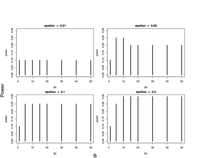
Figure 6: Power as a function of B and $\varepsilon$.

6.3 Linkage Weights

Finding variation in the genetic code that increases the risk for complex diseases, such as Type II diabetes and schizophrenia, is critically important to the advancement of genetic epidemiology. In theIntroduction we describe a means by which weights could be extracted from linkage data. Here we illustrate the idea with both data and simulations.

In the analysis of 955 cases and 1498 controls enrolled in a genome-wide association study, McQueen and colleagues (2008) used weights derived from published linkage results. They combined results from 11 linkage studies on bipolar disorder to obtain $Z$ scores corresponding to the locations of each association test. From the linkage results they computed weighted $p$-values using the cummulative normal weight function (Roeder et al., 2006). Although none of their results were genome-wide significant, they obtained promising results in four regions. Three of these are obtained due to strong $p$-values in combination with a linkage peak. One signal did not correspond to a linkage peak, but continued to be in the top tier of $p$-values, after weights were applied.

To illustrate how binary weights could be derived from such linkage data, we present a realistic synthetic example. Using the methods described inRoeder et al. (2006), we create a linkage trace that captures many of the features found in actual linkage traces. In this simulation we generate a full genome (23 chromosomes) and place 20 disease variants at random, one per chromosome. The signals from these variants were designed to yield weak signals with broad peaks. Next, we simulated 100,000 normally distributed association test statistics mapped to the same genome. Again, 20 of these tests were generated under the alternative hypothesis of association. These signals were also weak.

To illustrate the synthetic data, six typical chromosomes are displayed in Figure 1. Each displayed chromosome has one true signal, with the association test statistic at that location indicated by an upspike; none of the association tests generated under the null hypothesis are plotted. Without weights, only 2 of the 20 signals could be detected using a Bonferonni correction. Using binary weights, as described above, with $\varepsilon=0.05$ and $B=10$, we discover 5 of the 20 signals. In the left column of the figure all three signals were discovered, while in the right column none were discovered (indicated by presence of a down-spike). Comparing the top row, we see that both signals were up-weighted in the correct location, but the association signal was not strong enough in the top right chromosome to achieve significance. Alternatively, in the bottom left panel the association statistic was substantial enough to reject the null hypothesis without the benefit of up-weighting.

To examine the robustness of the procedure to choice of weights, we tried 4 choices of $\varepsilon$ (0.01, 0.05, 0.1, 0.2) with $1\leq B\leq 50$. We made no false discoveries with any of these choices. The power is displayed in Figure 6. To assist in the choice of parameters, we have found it helpful to examine the number of discoveries for each choice. In this example, the number of discoveries varied between 2 (unweighted, i.e., $B=1$) to 6 ($\varepsilon=0.2$, $B\geq 10$). Five discoveries were made for a broad range of choices. In principle, choosing $(\varepsilon,B)$ to maximize the number of discoveries can inflate the error rate. In our simulations we have found that searching within the family of weights defined by 1 or 2 parameters, such as this binary weight system based upon a linkage trace, tends to provide very close to nominal protection against false discoveries.

7 Discussion

Several authors have explored the effect of weights on the power of multiple testing procedures [e.g., Westfall, Kropf and Finos (2004)]. These investigations show that the power of multiple testing procedures can be increased by using weighted $p$-values. Here we derive the optimal weights for a commonly used family of tests and show that the power is remarkably robust to misspecification of these weights.

The same ideas used here can be applied to other testing methods to improve power. In particular,weights can be added to the FDR method, Holm’s stepdown test, and the Donoho and Jin (2004) method. Weighting ideas can also be used for confidence intervals. Another open question is the connection with Bayesian methods which have already been developed to some extent in Efron et al. (2001).

GWAS for some phenotypes such as Type 1 diabetes have yielded exciting results (Todd et al., 2007), while results for other complex diseases have been much less successful. Presumably, many studies do not have sufficient power to detect the genetic variants associated with the phenotypes, even though thousands of cases and controls have been genotyped. To bolster power, we recommend up-weighting and down-weighting hypotheses, based on prior likelihood of association with the phenotype. For instance, Wang, Li and Bucan (2007) describe pathway-based approaches for the analysis of GWAS.

Multiple testing arises in GWAS analyses in other contexts as well. Frequently, multiple tests, assuming different genetic models, are applied to each genetic marker. Multiple markers in a neighborhood can be analyzed simultaneously to increase the signal, using haplotypes, multivariate models and fine-mapping techniques. Data are often collected in multiple stages of the experiment, and at each stage promising markers are tested for association. In summary, many questions concerning multiple testing remain open in the context of GWAS.

Appendix

Proof of Lemma 2.1 The familywise error is

$$\mathbb{P}\bigl{(}(\mathcal{R}\cap\mathcal{H}_{0})>0\bigr{)} = \mathbb{P}\biggl{(}P_{j}\leq\frac{\alpha w_{j}}{m}\mbox{ for some }j\in\mathcal{H}_{0}\biggr{)}$$

$$\leq \sum_{j\in\mathcal{H}_{0}}\mathbb{P}\biggl{(}P_{j}\leq\frac{\alpha w_{j}}{m}\biggr{)}=\frac{\alpha}{m}\sum_{j\in\mathcal{H}_{0}}w_{j}$$

$$\leq \alpha\overline{w}=\alpha.$$

Proof of Lemma 2.2 The familywise error is

$$\mathbb{P}\bigl{(}(\mathcal{R}\cap\mathcal{H}_{0})>0\bigr{)}$$

$$\quad=\mathbb{P}\biggl{(}P_{j}\leq\frac{\alpha W_{j}}{m}\mbox{ for some }j\in\mathcal{H}_{0}\biggr{)}$$

$$\quad\leq\sum_{j\in\mathcal{H}_{0}}\mathbb{P}\biggl{(}P_{j}\leq\frac{\alpha W_{j}}{m}\biggr{)}$$

$$\quad=\sum_{j\in\mathcal{H}_{0}}\mathbb{E}_{H}\biggl{(}\mathbb{P}\biggl{(}P_{j}\leq\frac{\alpha w_{j}}{m}\Bigm{|}W_{j}=w_{j}\biggr{)}\biggr{)}$$

$$\quad=\sum_{j\in\mathcal{H}_{0}}\mathbb{E}_{H}(\alpha W_{j}/m)=\frac{\alpha}{m}\sum_{j\in\mathcal{H}_{0}}\mathbb{E}_{H}(W_{j})$$

$$\quad\leq\frac{m_{0}\alpha}{m}\leq\alpha.$$

Proof of Theorem 3.1 Let $C$ denote the set of hypotheses with $\xi_{j}>0$. Power is optimized if $w_{j}=0$ for $j\notin C$. The average power is

$$\frac{1}{m_{1}}\sum_{j\in C}{\overline{\Phi}}\biggl{(}{\overline{\Phi}^{-1}}\biggl{(}\frac{\alpha w_{j}}{m}\biggr{)}-\xi_{j}\biggr{)},$$

with constraint

$$\sum w_{j}=m.$$

Choose $\underline{w}$ to maximize

$$\pi=\frac{1}{m_{1}}\sum_{j\in C}{\overline{\Phi}}\biggl{(}{\overline{\Phi}^{-1}}\biggl{(}\frac{\alpha w_{j}}{m}\biggr{)}-\xi_{j}\biggr{)}-\lambda\Bigl{(}{m-\sum w_{i}}\Bigr{)}$$

by setting the derivative to zero

$$\frac{\partial}{\partial w_{i}}\pi = -\lambda+\frac{\phi({\overline{\Phi}^{-1}}(\alpha w_{j}/m)-\xi_{j})}{\phi({\overline{\Phi}^{-1}}(\alpha w_{j}/m))}\frac{\alpha}{m}=0,$$

$$\frac{m\lambda}{\alpha} = \frac{\phi({\overline{\Phi}^{-1}}(\alpha w_{j}/m)-\xi_{j})}{\phi({\overline{\Phi}^{-1}}(\alpha w_{j}/m))}.$$

The $\underline{w}$ that solves these equations is given in (3). Finally, solve for $c$ such that $\sum_{i}w_{i}=m$.

Proof of Theorem 3.4 The first statement follows easily by noting that the worst case corresponds to choosing weight $B$ in the first term in $R(\xi)$ and choosing weight $b$ in the second term in $R(\xi)$. The rest follows by Taylor expanding $R_{b,B}(\xi)$ around $b=1$.

Proof of Lemma 3.5 With $b=0$, $R_{b,B}(\xi)\geq 0$ when

$$\overline{\Phi}(z_{B\alpha/m}-\xi)-2\overline{\Phi}(z_{\alpha/m}-\xi)\geq 0.$$ (14)

With $B\geq 2$, (14) holds at $\xi=0$. The left-hand side is increasing in $\xi$ for $\xi$ near 0, but (14) does not hold at $\xi=z_{\alpha/m}$. So (14) must hold in the interval $[0,\xi_{*}]$. Rewrite (14) as $\overline{\Phi}(z_{B\alpha/m}-\xi)-\overline{\Phi}(z_{\alpha/m}-\xi)\geq\overline{\Phi}(z_{\alpha/m}-\xi)$. We lower bound the left-hand side and upper bound the right-hand side. The left-hand side is $\overline{\Phi}(z_{B\alpha/m}-\xi)-\overline{\Phi}(z_{\alpha/m}-\xi)=\int_{z_{B\alpha/m}-\xi}^{z_{\alpha/m}-\xi}\phi(u)\,du\geq(z_{\alpha/m}-z_{B\alpha/m})\phi(z_{\alpha/m}-\xi)$. The right-hand side can be bounded using Mill’s ratio: $\overline{\Phi}(z_{\alpha/m}-\xi)\leq\break\phi(z_{\alpha/m}-\xi)/(z_{\alpha/m}-\xi)$. Set the lower bound greater than the upper bound to obtain the stated result.

Proof of Lemma 3.6 Choose $K>1$ such that $1/(K+1)<1/a-\varepsilon$. Choose $1>\gamma>(2\alpha-a)/K$. Choose a small $c>0$. Let $\xi=A+\sqrt{A^{2}-2c}$ and $u=B-\sqrt{B^{2}-2c}$, where

$$A=\overline{\Phi}^{-1}\biggl{(}\frac{\alpha}{(m(\gamma K+a))}\biggr{)},$$

$$B=\overline{\Phi}^{-1}\biggl{(}\frac{K\alpha}{(m(\gamma K+a))}\biggr{)}.$$

Then $\rho(\xi)=1/a$ and $\tilde{\rho}(\xi)=1/(K+1)$. Now $d(Q,\break\tilde{Q})=\gamma$. Taking $K$ sufficiently large and $\gamma$ sufficiently close to $(2\alpha-a)/K$ makes $\gamma<\delta$.

It is convenient to prove Theorem 3.8 before proving Theorem 3.7.

Proof of Theorem 3.8 Let $c_{*}$ solve

$$\gamma\overline{\Phi}\bigl{(}\sqrt{2c_{*}}\bigr{)}+a\overline{\Phi}\biggl{(}\frac{\xi}{2}+\frac{c_{*}}{\xi}\biggr{)}=\frac{\alpha}{m}.$$ (15)

We claim first that, for any $c>c_{*}$, there is no $u$ such that the weights average to 1. Fix $c>c_{*}$. The weights average to 1 if and only if

$$\gamma\overline{\Phi}\biggl{(}\frac{c}{u}+\frac{u}{2}\biggr{)}+a\overline{\Phi}\biggl{(}\frac{\xi}{2}+\frac{c}{\xi}\biggr{)}=\frac{\alpha}{m}.$$ (16)

Since $c>c_{*}$ and since the second term is decreasing in $c$, we must have

$$\overline{\Phi}\biggl{(}\frac{c}{u}+\frac{u}{2}\biggr{)}>\overline{\Phi}\bigl{(}\sqrt{2c_{*}}\bigr{)}.$$

The function $r(u)=\overline{\Phi}(c/u+u/2)$ is maximized at $u=\sqrt{2c}$. So $r(\sqrt{2c})\geq r(u)$. But $r(\sqrt{2c})=\overline{\Phi}(\sqrt{2c})$. Hence, $\overline{\Phi}(\sqrt{2c})\geq r(u)\geq\overline{\Phi}(\sqrt{2c_{*}})$. This implies $c<c_{*}$, which is a contradiction. This establishes that $\sup_{u}c(u)\leq c_{*}$. On the other hand, taking $c=c_{*}$ and $u=\sqrt{2c_{*}}$ solves equation (16). Thus, $c_{*}$ is indeed the largest $c$ that solves the equation which establishes the first claim. The second claim follows by noting that

$$\gamma\overline{\Phi}\bigl{(}\sqrt{2c_{*}}\bigr{)}+a\overline{\Phi}\biggl{(}\frac{\xi}{2}+\frac{c_{*}}{\xi}\biggr{)}=\gamma\overline{\Phi}\bigl{(}\sqrt{2c_{*}}\bigr{)}+O(a).$$

Now set this expression equal to $\alpha/m$ and solve.

Proof of Theorem 3.7 Define $c_{*}$ as in (15). If $u_{*}=\sqrt{2c_{*}}\leq\xi$, then the the proof proceeds as in the previous proof. So we first need to establish for which values of $\xi$ is this true. Let $r(c)=\gamma\overline{\Phi}(\sqrt{2c})+a\overline{\Phi}(\xi/2+c/\xi)$. We want to find out when the solution of $r(c)=\alpha/m$ is such that $\sqrt{2c}\leq\xi$, or, equivalently, $c\leq\xi^{2}/2$. Now $r$ is decreasing in $c$. Since $\gamma+a\geq\alpha/m$, $r(-\infty)\geq\alpha/m$. Hence, there is a solution with $c\leq\xi^{2}/2$ if and only if $r(\xi^{2}/2)\leq\alpha/m$. But $r(\xi^{2}/2)=(\gamma+a)\overline{\Phi}(\xi),$ so we conclude that there is such a solution if and only if $(\gamma+a)\overline{\Phi}(\xi)\leq\alpha/m$, that is, $\xi\geq z_{\alpha/(m(\gamma+a))}=\xi_{0}$.

Now suppose that $\xi<\xi_{0}$. We need to find $u\leq\xi$ to make $c$ as large as possible in the equation $v(u,c)\equiv\gamma\overline{\Phi}(u/2+c/u)+a\overline{\Phi}(\xi/2+c/\xi)=\alpha/m$. Let $u_{*}=\xi$ and $c_{*}=\xi z_{\alpha/(m(\gamma+a))}-\xi^{2}/2$. By direct substitution, $v(u_{*},c_{*})=\alpha/m$ for this choice of $u$ and $c$ and, clearly, $u_{*}\leq\xi$ as required. We claim that this is the largest possible $c_{*}$. To see this, note that $v(u,c)<v(u,c_{*})$. For $\xi\leq\xi_{0}$, $v(u,c_{*})$ is a decreasing function of $u$. Hence, $v(u,c)<v(u,c_{*})\leq v(u_{*},c_{*})=\alpha/m$. This contradicts the fact that $v(u,c)=\alpha/m$.

For the second claim, note that the power of the weighted test beats the power of Bonferroni if and only if the weight $w=(m/\alpha)\overline{\Phi}(\xi/2+C(\xi)/2)\geq 1$, which is equivalent to

$$C(\xi)\leq\xi z_{\alpha/m}-\xi^{2}/2.$$ (17)

When $\xi\leq\xi_{0}$, $C(\xi)=\xi\xi_{0}-\xi^{2}/2$. By assumption, $\gamma+a\leq 1$ so that $z_{\alpha/(m(\gamma+a))}\leq z_{\alpha/m}$ and now suppose that $\xi_{0}<\xi\leq\xi_{*}$. Then $C(\xi)$ is the solution to $r(c)=\gamma\overline{\Phi}(\sqrt{2c})+a\overline{\Phi}(\xi/2+c/\xi)=\alpha/m$. We claim that (17) still holds. Suppose not. Then, since $r(c)$ is decreasing in $c$, $r(\xi z_{\alpha/m}-\xi^{2}/2)>r(C(\xi))=\alpha/m$. But, by direct calculation, $r(\xi z_{\alpha/m}-\xi^{2}/2)>\alpha/m$ implies that $\xi>\xi_{*}$, which is a contradiction. Thus, (7) holds.

Finally, we turn to (8). In this case, $C(\xi)=z^{2}_{\alpha/(m\gamma)}/\break 2+O(a)$. The worst case power is $\overline{\Phi}(C(\xi)/\xi-\xi/2)=\overline{\Phi}(z^{2}_{\alpha/(m\gamma)}/(2\xi)-\xi/2)+O(a)$. The latter is increasing in $\xi$ and so is at least $\overline{\Phi}(z^{2}_{\alpha/(m\gamma)}/(2\xi_{*})-\xi_{*}/2)+O(a)=\overline{\Phi}((z^{2}_{\alpha/(m\gamma)}/(2\xi_{*})-\xi_{*}^{2})/(2\xi_{*}))+O(a)$, asclaimed. The next two equations follow from standard tail approximations for Gaussians. Specifically, a Gaussian quantile $z_{\beta/m}$ can be written as $z_{\beta/m}=\sqrt{2\log(mL_{m}/\beta)}$, where $L_{m}=c\log^{a}(m)$ for constants $a$ and $c$ [Donoho and Jin (2004)]. Inserting this into the previous expression yields the final expression.

Proof of Theorem 4.2 Setting $\pi(w,\xi_{m})=\overline{\Phi}(\overline{\Phi}^{-1}(w\alpha/m)-\xi_{m})$ equal to $1-\beta$ implies $w=(m/\alpha)\overline{\Phi}(z_{1-\beta}+z_{\alpha/m})$, which is equal to $w_{1}$ as stated in the theorem. The stated form of $w_{0}$ implies that the weights average to 1. The stated solution thus satisfies the restriction that a fraction $\varepsilon$ have power at least $1-\beta$. Increasing the weight of any hypothesis whose weight is $w_{0}$ necessitates reducing the weight of another hypothesis. This either reduces the minimum power or forces a hypothesis with power $1-\beta$ to fall below $1-\beta$. Hence, the stated solution does in fact maximize the minimum power.

References

- Benjamini and Hochberg (1995) Benjamini, Y. and Hochberg, Y. (1995). Controlling the false discovery rate: A practical and powerful approach to multiple testing. J. Roy. Statist. Soc. Ser. B 57 289–300. \MR1325392
- Benjamini and Hochberg (1997) Benjamini, Y. and Hochberg, Y. (1997). Multiple hypotheses testing with weights. Scand. J. Statist. 24 407–418. \MR1481424
- Benjamini, Krieger and Yekutieli (2006) Benjamini, Y., Krieger, A. M. and Yekutieli, D. (2006). Adaptive linear step-up procedures that control the false discovery rate. Biometrika 93 491–507. \MR2261438
- Benjamini and Yekutieli (2001) Benjamini, Y. and Yekutieli, D. (2001). The control of the false discovery rate in multiple testing under dependency. Ann. Statist. 29 1165–1188. \MR1869245
- Bickel et al. (1993) Bickel, P., Klaassen, C., Ritov, Y. and Wellner, J. (1993). Efficient and adaptive estimation for semiparametric models. Technical report, Johns Hopkins Series in the Mathematical Statistics, Baltimore, Maryand. \MR1245941
- Blanchard and Roquain (2008) Blanchard, G. and Roquain, E. (2008). Two simple sufficient conditions for FDR control. Electron. J. Stat. 2 963–992. \MR2448601
- Blanchard and Roquain (2009) Blanchard, G. and Roquain, E. (2009). Adaptive FDR control under independence and dependence. J. Mach. Learn. Res. To appear.
- Chen et al. (2000) Chen, J. J., Lin, K. K., Huque, M. and Arani, R. B. (2000). Weighted -value adjustments for animal carcinogenicity trend test. Biometrics 56 586–592.
- Donoho and Jin (2004) Donoho, D. and Jin, J. (2004). Higher criticism for detecting sparse heterogeneous mixtures. Ann. Statist. 32 962–994. \MR2065195
- Efron (2007) Efron, B. (2007). Simultaneous inference: When should hypothesis testing problems be combined? Ann. Appl. Statist. 2 197–223. \MR2415600
- Efron et al. (2001) Efron, B., Tibshirani, R., Storey, J. D. and Tusher, V. (2001). Empirical Bayes analysis of a microarray experiment. J. Amer. Statist. Assoc. 96 1151–1160. \MR1946571
- Genovese and Wasserman (2002) Genovese, C. and Wasserman, L. (2002). Operating characteristics and extensions of the false discovery rate procedure. J. R. Stat. Soc. Ser. B Stat. Methodol. 64 499–517. \MR1924303