ITFA-2010-05

The Volume Conjecture,
Perturbative Knot Invariants,
and
Recursion Relations for Topological Strings

Robbert Dijkgraaf¹, Hiroyuki Fuji² and Masahide Manabe³

¹ Institute for Theoretical Physics $\&$ KdV Institute for Mathematics
University of Amsterdam, Spui 21, 1012 WX Amsterdam, The Netherlands
² Department of Physics, Nagoya University, Nagoya 464-8602, Japan
³ Graduate School of Mathematics, Nagoya University, Nagoya 464-8602, Japan

Abstract

We study the relation between perturbative knot invariants and the free energies defined by topological string theory on the character variety of the knot. Such a correspondence between $SL(2;\mathbb{C})$ Chern-Simons gauge theory and the topological open string theory was proposed earlier on the basis of the volume conjecture and AJ conjecture. In this paper we discuss this correspondence beyond the subleading order in the perturbative expansion on both sides. In the computation of the perturbative invariants for the hyperbolic 3-manifold, we adopt the state integral model for the hyperbolic knots, and the factorized AJ conjecture for the torus knots. On the other hand, we iteratively compute the free energies on the character variety using the Eynard-Orantin topological recursion relation. We check the correspondence for the figure eight knot complement and the once punctured torus bundle over $\mathbb{S}^{1}$ with the holonomy $L^{2}R$ up to the fourth order. For the torus knots, we find trivial the recursion relations on both sides.

1 Introduction

Three-dimensional Chern-Simons gauge theory is one of the most widely studied topological quantum field theories. It has found many applications in physics and mathematics. In the celebrated paper by Witten [1] a relation between the Chern-Simons gauge theory and knot invariants was discovered, and it was shown that the expectation value of the Wilson loop operator along the knot on 3-sphere $\mathbb{S}^{3}$ and the colored Jones polynomial are equivalent.

Another remarkable aspect of the Chern-Simons gauge theory is its relation with theories of three-dimensional quantum gravity [2]. When gravity in three dimensions is reformulated in the first order formalism, it also yields a Chern-Simons gauge theory. In particular, in this approach $SL(2;\mathbb{C})$ Chern-Simons gauge theory becomes equivalent to the Euclidean signature quantum gravity with a negative cosmological constant. In the classical limit this corresponds to the study of the hyperbolic structures. Connecting these two aspects of the Chern-Simons gauge theory, led to the volume conjecture as originally proposed by Kashaev [3].

The volume conjecture concerns the asymptotic behavior of the colored Jones polynomial [4]. Let $J_{n}(K;q)$ be the $n$-colored Jones polynomial for a hyperbolic knot $K$. The claim of the volume conjecture is [3, 4]:

$$\frac{1}{\pi}\lim_{n\to\infty}\frac{|\log J_{n}(K;q=e^{2\pi i/n})|}{n}={\rm Vol}(\mathbb{S}^{3}\backslash K),$$ (1.1)

where ${\rm Vol}(\mathbb{S}^{3}\backslash K)$ is the hyperbolic volume of the knot complement. The volume conjecture has been extended to the complexified version [4], and further generalized to knot complements with the deformed hyperbolic structure [5]. The volume conjecture beyond the leading order was discussed firstly in [6]. The subleading term in the asymptotic expansion of the colored Jones polynomial coincides with the Reidemeister torsion [7].

In previous work [8], two of the authors proposed a correspondence between $SL(2;\mathbb{C})$ Chern-Simons gauge theory and the topological open string theory. This correspondence was suggested by a similar set-up in the two problems. Let us briefly review this argument.

If $M$ is the three-manifold obtained by removing a tubular neighbourhood of the knot $K$, then any quantum field theory on $M$ will produce a quantum state $Z(M)$ in the Hilbert space associated to the boundary $\partial M$ of $M$. In the case of a knot complement, the boundary has the topology $\partial M\cong\mathbb{T}^{2}$. Semi-classically, the state $Z(M)$ is described by a Lagrangian sub-manifold in the phase space associated to the boundary. For $SL(2;\mathbb{C})$ Chern-Simons gauge theory the classical phase space can be identified with the space of gauge equivalence classes of the flat $SL(2;\mathbb{C})$ connections on $\mathbb{T}^{2}$. The Lagrangian corresponding to $M$ is the character variety $\cal C$ of the knot $K$, defined as the set of connections on $\mathbb{T}^{2}$ that extend as flat connections over $M$ [9]. The character variety is an algebraic curve in (a quotient of) $\mathbb{C}^{*}\times\mathbb{C}^{*}$ equipped with its canonical symplectic structure. We can pick a local coordinate $u$ on the curve $\cal C$, which can be identified with the free monodromy around the meridian of the knot. The full CS partition function or knot invariant now corresponds to the full quantum wave function $Z(M;u)$.

This set-up of an algebraic curve $\cal{C}\subset\mathbb{C}^{*}\times\mathbb{C}^{*}$ appears also in the topological string theory. In this case we considered the toric Calabi-Yau 3-fold $X$ which can be regarded as a fibration over the character variety of the knot. In this case the Riemann surface is usually called the spectral curve. If we add a topological D-brane in this CY variety, the open string partition function will also be a wave function $Z(X;u)$. So, in both the Chern-Simons gauge theory and the topological string theory we quantize the character variety. The conjecture that we study further in this paper is that, with a suitable identification, these quantizations are equivalent, i.e., we have

$$Z(M;u)=Z(X;u).$$ (1.2)

This correspondence is summarized in more detail in the following table. The various notations that we use here, will become clear in the subsequent.

3D Chern-Simons	Topological Open String
$u=2\pi i\left(\frac{n}{k}-1\right)$: Meridian holonomy	$u$: Area of holomorphic disk
$q=e^{2\pi i/k}$	$q=e^{g_{s}}$
Vol+$i$CS	Disk free energy ${\cal F}^{(0,1)}$
Reidemeister torsion	Annulus free energy ${\cal F}^{(0,2)}$
AJ conjecture	Quantum Riemann Surface
${A}_{K}(\hat{m},\hat{\ell};q)J_{n}(K;q)=0$	$\hat{H}(e^{-u-g_{s}/2},e^{g_{s}\partial_{u}};q)Z_{\rm open}(u;q)=0$
$\hat{m}\hat{\ell}=q^{1/2}\hat{\ell}\hat{m}$	$e^{-u-g_{s}/2}e^{g_{s}\partial_{u}}=q^{1/2}e^{g_{s}\partial_{u}}e^{-u-g_{s}/2}$

This correspondence is checked explicitly for two examples, the figure eight knot complement and the once punctured torus bundle over $\mathbb{S}^{2}$ with the holonomy $L^{2}R$, which is isomorphic to the SnapPea census manifold $m009$ [10], which is the complement of a knot in a three-manifold of different topology than the three-sphere [11, 12, 13]. Up to subleading order, one can find coincidence for these examples.

On the other hand, in [14, 15] it is conjectured that the free energies of the topological (A-type) open string theory on toric Calabi-Yau 3-folds with toric branes are iteratively obtained by the Eynard-Orantin topological recursion relation [16]. The recursion relation is applicable for any complex plane curve, and in the topological string theory, via the mirror symmetry, the open string moduli are described by the mirror curve which is a complex plane curve in ${\mathbb{C}}^{*}\times{\mathbb{C}}^{*}$. These recursions can be derived as the Schwinger-Dyson equations in two dimensional Kodaira-Spencer theory, the theory of a chiral boson on the mirror curve [17]. The techniques of the computation are developed in [18, 19, 20]. In this paper, we discuss our correspondence to the higher orders beyond the subleading order in the topological expansion of the free energies of the topological open string theory. To this end we define the BKMP’s free energies according to remodeling the B-model [14, 15], and compute them for the character variety of the hyperbolic manifold up to the fifth order in the recursions, in the case of the above two examples.

On the Chern-Simons gauge theory side, the higher order perturbative invariants are computed in [21, 22]. For the figure eight knot complement we can compute the perturbative invariant from the colored Jones polynomial. But for the once punctured torus bundle the complete form of the colored Jones polynomial is not known. To analyze such manifolds, we adopt the state integral model which is constructed in [23, 24, 25, 21]. The partition function of the state integral model for a simplicially decomposed hyperbolic 3-manifold gives topological invariants like the Ponzano-Regge [26] and the Turaev-Viro models [27]. In this paper, we compute the perturbative invariants from the state integral model, and compare them with the free energy on the character variety.

As a result of these computations, we find some discrepancies between the perturbative invariants and the BKMP’s free energy of the topological string in the higher order. These discrepancies may come from the choice of the integration path in the computation of the free energy in the B-model or ${\cal O}(g_{s})$ modification of the Calabi-Yau geometry [28, 29, 30]. To remedy this point, we consider some regularization for the constant $G$ which appears in the Bergman kernel, because the constant $G$ changes under the monodromy transformation of the genus one character variety. Although the regularization would be ad-hoc, we find the regularization rules for $G^{n}$ terms in the recursions up to the fourth order. After the regularization, we recover the perturbative invariants of the state integral model for the above two examples non-trivially.

For the case of torus knots, the colored Jones polynomial is well-studied. We can extract the perturbative invariants adopting the $q$-difference equation which is called the AJ conjecture [31, 32, 33, 34, 35]. Compared to the state integral model, there exist two branches which correspond to abelian and non-abelian representations of the $PSL(2;\mathbb{C})$ holonomy along the meridian for the colored Jones polynomial. In this paper we will compare the perturbative invariants for the non-abelian branch and the BKMP’s free energy on the character variety. In this class of knots we find that the perturbative invariants and BKMP’s free energies are trivial as the $u$-dependent functions, and we can check our correspondence to all orders in the perturbative expansion.

The organization of this paper is as follows. In section 2, after a short summary of the state integral model, we show the explicit computation for the figure eight knot complement and the once punctured torus bundle over $\mathbb{S}^{1}$ with the holonomy $L^{2}R$. The computation of the figure eight knot complement was already given in [21], and the second example is novel. In section 3, we turn to the computation of the BKMP’s free energies on the character variety. In this section, we firstly derive the general solution of the topological recursion relations for the two branched plane curve with genus one up to the fourth order. And then we apply the formula to the character varieties for the figure eight knot complement and the once punctured torus bundle over $\mathbb{S}^{1}$ with the holonomy $L^{2}R$. The correspondence for the torus knots is discussed in section 4. In appendix A, we discuss the AJ conjecture. We explicitly see the factorization of the $q$-difference equation for the figure eight knot, and summarize the computation of the perturbative invariants for some torus knots in the abelian branch. In appendix B, we summarize the details of the derivations of the general formula for the fourth order terms $W^{(0,4)}$ and $W^{(1,2)}$. In appendix C, we show the computation on the annulus free energy ${\cal F}_{1}(p)$. In appendix D, the computational result of the fifth order free energy ${\cal F}_{4}(p)$ is summarized.

2 Asymptotic expansion for the state integral model

The volume conjecture describes the asymptotic behavior of the colored Jones polynomial. To evaluate the saddle point value perturbatively, the information of the cyclotomic expansion of the colored Jones polynomial is necessary because we use a $q$-difference equation in the analysis. In general it is not an easy task to obtain such an expansion. In particular for the once punctured torus bundle over $\mathbb{S}^{1}$, the original colored Jones polynomial can not be found, although the simplicial decomposition is realized explicitly.

The partition function of the state integral model [23, 24, 25] on the hyperbolic $3$-manifold gives the topological invariant. The asymptotic expansion of the partition function is computable only from the information of the simplicial decomposition via ideal tetrahedra. For the figure eight knot, the asymptotic expansions of the partition function of the state integral model and the colored Jones polynomial are computed thoroughly in [21], and both of them give the same expansions. In this section, we evaluate the asymptotic expansion of the state integral model based on the method which is developed in [21].

2.1 State integral model

Here we briefly summarize about the state integral model. For a hyperbolic knot complement, the simplicial decomposition with the ideal tetrahedra can be performed [36]. There are two kinds of ideal tetrahedra with an orientation $\varepsilon=\pm 1$. For each face of the tetrahedron, a vector space $V$ or its dual $V^{*}$ is assigned corresponding to the orientation. The vector space $V$ is the Hilbert space of the Heisenberg algebra with continuum eigenvalue for the momentum operator:

$$[\hat{q},\hat{p}]=2\hbar,$$ (2.1)

$$\hat{p}|p\rangle=p|p\rangle,\quad|p\rangle\in V.$$ (2.2)

Thus a tensor product of the vector spaces $V\otimes V\otimes V^{*}\otimes V^{*}$ is assigned for an ideal tetrahedron.

As a weight of the state integral model, one can choose the matrix element of the operator ${\bf S}\in{\rm Hom}_{\mathbb{C}}(V\otimes V,V\otimes V)$. To acquire topological invariance for the partition function, the operator should satisfy the pentagon relation on $V_{1}\otimes V_{2}\otimes V_{3}$:

$${\bf S}_{2,3}{\bf S}_{1,2}={\bf S}_{1,2}{\bf S}_{1,3}{\bf S}_{2,3},$$ (2.3)

where ${\bf S}_{i,j}$ acts on $V_{i}\otimes V_{j}$. In state integral model [23, 25], the operator ${\bf S}$ which satisfy the above pentagon relation on the infinite dimensional momentum space $|p\rangle$ is defined on $V_{1}\otimes V_{2}$ as:

$${\bf S}_{1,2}=e^{\hat{q}_{1}\hat{p}_{1}/2\hbar}\Phi_{\hbar}(\hat{p}_{1}+\hat{q}_{2}-\hat{p}_{2}),$$ (2.4)

where $\Phi_{\hbar}(p)$ is the quantum dilogarithm function. For $i\hbar\in\mathbb{R}$ and $|{\rm Im}\;p|<\pi$, the function $\Phi_{\hbar}(p)$ is given by the Faddeev’s integral formula [37]:

$$\Phi_{\hbar}(p)=\exp\left[\frac{1}{4}\int_{\mathbb{R}+i0}\frac{dx}{x}\frac{e^{-ipx}}{\sinh(i\hbar x)\sinh(\pi x)}\right].$$ (2.5)

Because this Faddeev integral fulfills the pentagon relation:

$$\Phi_{\hbar}(\hat{p})\Phi_{\hbar}(\hat{q})=\Phi_{\hbar}(\hat{q})\Phi_{\hbar}(\hat{p}+\hat{q})\Phi_{\hbar}(\hat{p}),$$ (2.6)

the pentagon relation (2.3) for ${\bf S}$ operators is implied.

The ${\bf S}$-matrix elements for the ideal tetrahedra of $\varepsilon=\pm 1$ as in Fig.1 are obtained as follows:

$$\langle p_{1}^{(-)},p_{2}^{(-)}|{\bf S}|p_{1}^{(+)},p_{2}^{(+)}\rangle = \frac{\delta\big{(}p_{1}^{(-)}+p_{2}^{(-)}-p_{1}^{(+)}\big{)}}{\sqrt{4\pi\hbar/i}}\Phi_{\hbar}(p_{2}^{(+)}-p_{2}^{(-)}+i\pi+\hbar)$$ (2.7)

$$\times e^{\frac{1}{2\hbar}\left[p_{1}^{(-)}(p_{2}^{(+)}-p_{2}^{(-)})+\frac{i\pi\hbar}{2}-\frac{\pi^{2}-\hbar^{2}}{6}\right]},$$

$$\langle p_{1}^{(-)},p_{2}^{(-)}|{\bf S}^{-1}|p_{1}^{(+)},p_{2}^{(+)}\rangle = \frac{\delta\big{(}p_{1}^{(-)}-p_{1}^{(+)}-p_{2}^{(+)}\big{)}}{\sqrt{4\pi\hbar/i}}\frac{1}{\Phi_{\hbar}(p_{2}^{(-)}-p_{2}^{(+)}-i\pi-\hbar)}$$ (2.8)

$$\times e^{\frac{1}{2\hbar}\left[-p_{1}^{(+)}(p_{2}^{(-)}-p_{2}^{(+)})-\frac{i\pi\hbar}{2}+\frac{\pi^{2}-\hbar^{2}}{6}\right]}.$$

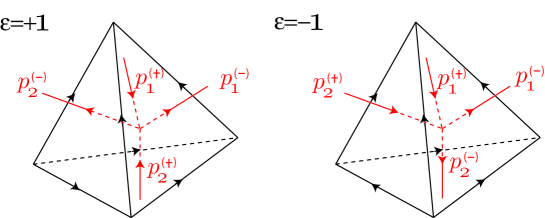
Figure 1: Ideal tetrahedra of different orientation

The partition function for the state integral model on a 3-manifold $M$ with the complete hyperbolic structure is defined by

$$Z_{\hbar}(M;\hbar,0)=\sqrt{2}\int d{\bf p}\delta_{C}({\bf p})\delta_{G}({\bf p})\prod_{i=1}^{N}\langle p_{2i-1}^{(-)},p_{2i}^{(-)}|{\bf S}^{\varepsilon_{i}}|p_{2i-1}^{(+)},p_{2i}^{(+)}\rangle,$$ (2.9)

where ${\bf p}$ is a set of $(p_{2i-1}^{(\varepsilon_{i})},p_{2i}^{(\varepsilon_{i})})$. The delta functions $\delta_{G}({\bf p}):=\prod\delta\big{(}p_{j}^{(-)}-p_{k}^{(+)}\big{)}$ and $\delta_{C}({\bf p})$ imply the gluing condition for the faces and the complete gluing condition for the triangles on the boundary $\partial M\simeq\mathbb{T}^{2}$ respectively. The asymptotic behavior of this invariant is studied for various knot complements [23, 25].

The partition function for the 3-manifold with the deformed complete structure is also considered [21]. The deformation of the completeness condition changes one of the delta functions in $\delta_{C}({\bf p})$ with $\delta(\sum p_{i}=2u)$. In this delta function, the sum is taken for the momenta which appear in the shape parameters $z_{i}=e^{p_{2i}^{(+)}-p_{2i-1}^{(-)}}$ of the ideal tetrahedra along the meridian of the boundary torus [24]. As a result of this deformation, one finds a holonomy representation along the meridian $\mu$:

$$\rho(\mu)=\left(\begin{array}[]{cc}m&*{}\\ 0&m^{-1}\end{array}\right),\quad m=e^{u}.$$ (2.12)

Under this deformation, the partition function yields

$$Z_{\hbar}(M;\hbar,u) = \sqrt{2}e^{-u}\int d{\bf p}\delta_{C}({\bf p};u)\delta_{G}({\bf p})\prod_{i=1}^{N}\langle p_{2i-1}^{(-)},p_{2i}^{(-)}|{\bf S}^{\varepsilon_{i}}|p_{2i-1}^{(+)},p_{2i}^{(+)}\rangle$$ (2.13)

$$= \sqrt{2}\int\prod_{j=1}^{N-1}\frac{dp_{j}}{\sqrt{4\pi\hbar}}\prod_{i=1}^{N}\Phi_{\hbar}\left(g_{i}({\bf p},2u)+\varepsilon_{i}(i\pi+\hbar)\right)^{\varepsilon_{i}}e^{\frac{1}{2\hbar}f({\bf p},2u,\hbar)-u},$$

where $g_{i}({\bf p},2u)$ is a linear function of ${\bf p}$, and $f({\bf p},2u,\hbar)$ is a quadratic polynomial.

Although the contour of the integrations of the partition function is not defined explicitly, the WKB expansion around the saddle point is computable [21]. In the limit $\hbar\to 0$, the partition function (2.13) is approximated by

$$Z_{\hbar}(M;\hbar,u)\sim\int d{\bf p}\;e^{\frac{1}{\hbar}V({\bf p},u)},\quad\hbar\to 0,$$ (2.14)

$$V({\bf p},u)=\frac{1}{2}\sum_{i=1}^{N}\varepsilon_{i}{\rm Li}_{2}\left(-\exp(g_{i}({\bf p},2u)+i\pi\varepsilon_{i})\right)+\frac{1}{2}f({\bf p},2u,\hbar=0).$$ (2.15)

The saddle point conditions

$$\frac{\partial V({\bf p},u)}{\partial p_{j}}=0$$ (2.16)

for all $j$ specify the saddle point ${\bf p}$. There may exist several saddle points for a hyperbolic 3-manifold $M$, and the value of the partition function may differ for each branch. In the following, we discuss only the geometric branch. For the general saddle point values, the face angles of the ideal tetrahedra which is determined by a shape parameters may become non-geometric [36, 38]. In the geometric branch, all of the ideal tetrahedra in the simplicial decomposition are geometric and completely glued. The saddle point value of the potential $V({\bf p},u)$ will satisfy $V({\bf p}_{0},u=0)=i{\rm Vol}(M)-{\rm CS}(M)$. This property is the same as the volume conjecture [3, 4], and it is expected that the perturbative invariants for the state integral model will coincide with those of colored Jones polynomial.

In [25] it is proposed that the potential function $V({\bf p}_{0},u)$ is identified with the Neumann-Zagier potential [39]. The Neumann-Zagier potential satisfies a relation:

$$\frac{\partial}{\partial u}V({\bf p}_{0},u)=v,$$ (2.17)

where $l:=e^{v}$ is an eigenvalue of the holonomy representation $\rho(\nu)$ along the longitude $\nu$ of the boundary $\partial M$. This condition imposes a non-trivial constraint on $(l,m)\in\mathbb{C}^{*}\times\mathbb{C}^{*}$. By the saddle point equation (2.16) one can eliminate ${\bf p}$ and find an algebraic equation:

$$A_{K}(l,m)=0.$$ (2.18)

The polynomial $A_{K}(l,m)$ coincides with the A-polynomial which is reciprocal $A_{K}(l,m)=l^{a}m^{b}A_{K}(l^{-1},m^{-1})$. Then the saddle point value of the potential $V({\bf p},u)$ will satisfy the generalized volume conjecture $V({\bf p}_{0},u)=i{\rm Vol}(M,u)-{\rm CS}(M,u)$ [5].

The higher order terms in the expansion around the saddle point is evaluated by the following expansion of the quantum dilogarithm function:

$$\Phi_{\hbar}(p_{0}+p) = \exp\bigg{[}\sum_{n=0}^{\infty}B_{n}\Big{(}\frac{p}{2\hbar}+\frac{1}{2}\Big{)}{\rm Li}_{2-n}(-e^{p_{0}})\frac{(2\hbar)^{n-1}}{n!}\bigg{]},$$ (2.19)

where the Bernoulli polynomial $B_{n}(x)=\sum_{k=0}^{n}{}_{n}C_{k}B_{k}x^{n-k}$ satisfies $B_{n}^{\prime}(x)=nB_{n-1}(x)$. Plugging this expansion into (2.13), one can expand the partition function $Z_{\hbar}(M;\hbar,u)$ around the saddle point ${\bf p}_{0}$ as:

$$Z_{\hbar}(M;\hbar,u)=\exp\bigg{[}\frac{1}{\hbar}S_{0}(u)+\sum_{n=0}^{\infty}S_{n+1}(u)\hbar^{n}\bigg{]},\quad S_{0}(u)=V({\bf p}_{0},u).$$ (2.20)

In the following, we will compute the higher order terms in the saddle point approximation for the figure eight knot complement [21] and the once puncture torus bundle over $\mathbb{S}^{1}$ with the holonomy $L^{2}R$.

2.2 Perturbative expansion for figure eight knot complement

As the first example we summarize the computation for the figure eight knot complement [25, 21]. The figure eight knot complement can be decomposed into two ideal tetrahedra with the different orientations [36]. The partition function for the state integral model yields

$$Z_{\hbar}(\mathbb{S}^{3}\backslash{\bf 4_{1}};\hbar,u)=\sqrt{2}e^{-u}\int d{\bf p}\delta_{C}({\bf p},u)\langle p_{1},p_{2}|S|p_{3},p_{4}\rangle\langle p_{4},p_{3}|S^{-1}|p_{2},p_{1}\rangle.$$ (2.21)

The shape parameters $z_{1}=e^{p_{4}-p_{2}}$ and $z_{2}=e^{p_{1}-p_{3}}$ satisfies the meridian condition $z_{1}z_{2}^{-1}=e^{-2u}$, and the delta function $\delta_{C}({\bf p};u)$ has the support on

$$p_{4}-p_{2}-(p_{1}-p_{3})=-2u.$$ (2.22)

Evaluating some of the integrals in (2.21) one obtains

$$Z_{\hbar}(\mathbb{S}^{3}\backslash{\bf 4_{1}};\hbar,u)=\frac{1}{\sqrt{2\pi\hbar}}\int_{C}dp\frac{\Phi_{\hbar}(p+i\pi+\hbar)}{\Phi_{\hbar}(-p-2u-i\pi-\hbar)}e^{-\frac{2}{\hbar}u(u+p)-u}.$$ (2.23)

Since the figure eight knot is fully amphichiral, the term $i\pi+\hbar$ in the argument of the quantum dilogarithm can be removed by shifting $p\to p-u-i\pi-\hbar$. This shift of the variable changes the integration path ${C}$. Although such shift gives rise to the corrections of order $e^{-{\rm const}/\hbar}$ to $Z_{\hbar}$, the higher order terms $S_{n}$ ($n=1,\ldots$) are not affected.

Under the shift of the variable $p\to p-u-i\pi-\hbar$, the partition function of the state integral model simplifies

$$Z(\mathbb{S}^{3}\backslash{\bf 4_{1}};\hbar,u) = \frac{1}{\sqrt{2\pi\hbar}}e^{\frac{2\pi iu}{\hbar}+u}\int_{C}dp\frac{\Phi_{\hbar}(p-u)}{\Phi_{\hbar}(-p-u)}$$ (2.24)

$$= \frac{1}{\sqrt{2\pi\hbar}}e^{\frac{2\pi iu}{\hbar}+u}\int_{C}dp\;e^{\Upsilon(\hbar,p,u)},$$

where one can compute the expansion of the function $\Upsilon(\hbar,p,u)$ adopting (2.19) as:

$$\Upsilon(\hbar,p_{0}+p,u)=\sum_{j=0}^{\infty}\sum_{k=-1}^{\infty}\Upsilon_{j,k}(p,u)p^{j}\hbar^{k},$$ (2.25)

$$\Upsilon_{j,k}=\frac{B_{k+1}(1/2)2^{k}}{(k+1)!j!}\left[{\rm Li}_{1-j-k}(-e^{p-u})-(-1)^{j}{\rm Li}_{1-j-k}(-e^{-p-u})\right].$$ (2.26)

In the following, we will evaluate $Z(\mathbb{S}^{3}\backslash{\bf 4_{1}};\hbar,u)$ on the geometric branch. In this branch, the saddle point value of $p_{0}$ is

$$p_{0}=p^{({\rm geom})}(u)=\log\bigg{[}\frac{1-m^{2}-m^{4}-m^{2}\Delta(m)}{2m^{3}}\bigg{]},$$ (2.27)

$$\Delta(m)=\sqrt{m^{-4}-2m^{-2}-1-2m^{2}+m^{4}}.$$ (2.28)

The perturbative invariants $S_{n}(u)$ are computed systematically by evaluating the Gaussian integrals,

$$Z_{\hbar}(\mathbb{S}^{3}\setminus{\bf 4_{1}};\hbar,u)=\frac{e^{u+\frac{1}{\hbar}V(u)}}{\sqrt{2\hbar}}\int_{C}dp\;e^{-\frac{b(u)}{2\hbar}p^{2}}\exp\bigg{[}\frac{1}{\hbar}\sum_{j=3}^{\infty}\Upsilon_{j,-1}p^{j}+\sum_{j=0}^{\infty}\sum_{k=1}^{\infty}\Upsilon_{j,k}\hbar^{k}p^{j}\bigg{]}.$$ (2.29)

In the geometric branch, the first two terms yield

$$S_{0}=V(u)=\frac{1}{2}\Big{[}{\rm Li}_{2}(-e^{p^{({\rm geom})}-u})-{\rm Li}_{2}(-e^{-p^{({\rm geom})}-u})-4p^{({\rm geom})}u+4\pi iu\Big{]},$$ (2.30)

$$S_{1}=-\frac{1}{2}\log\frac{b(u)}{m^{2}}=-\frac{1}{2}\log[i\Delta(m)/2],$$ (2.31)

The result $S_{1}(u)$ is consistent with the Reidemeister torsion of $\mathbb{S}^{3}\backslash{\bf 4_{1}}$ [7, 6]. The A-polynomial is computed from the equations (2.16) and (2.17) with $S_{0}(u)=V(u)$,

$$A_{\bf 4_{1}}(l,m)=-m^{4}+l(1-m^{2}-2m^{4}-m^{6}+m^{8})-l^{2}m^{4}.$$ (2.32)

The higher order terms are computed in the same way:

$$S_{2}=\frac{15}{2b^{3}}\Upsilon_{3,-1}^{2}+\frac{3}{b^{2}}\Upsilon_{4,-1}+\Upsilon_{0,1},$$ (2.33)

$$S_{3}=\frac{3465}{8b^{6}}\Upsilon_{3,-1}^{4}+\frac{945}{2b^{5}}\Upsilon_{3,-1}^{2}\Upsilon_{4,-1}+\frac{105}{2b^{4}}\left(2\Upsilon_{3,-1}\Upsilon_{5,-1}+\Upsilon_{4,-1}^{2}\right)$$

$$\hskip 28.45274pt+\frac{15}{2b^{3}}\left(2\Upsilon_{6,-1}+\Upsilon_{0,1}\Upsilon_{3,-1}^{2}\right)+\frac{3}{b^{2}}\left(\Upsilon_{0,1}\Upsilon_{4,-1}+\Upsilon_{1,1}\Upsilon_{3,-1}\right)$$

$$\hskip 28.45274pt+\frac{1}{b}\Upsilon_{2,1}+\Upsilon_{0,2}+\frac{1}{2}\Upsilon_{0,1}^{2}-\frac{S_{2}^{2}}{2},$$ (2.34)

$$S_{4}=\frac{1}{24b^{7}}\left(810810\Upsilon_{3,-1}^{2}\Upsilon_{4,-1}^{2}+540540\Upsilon_{3,-1}^{3}\Upsilon_{5,-1}\right)$$

$$\hskip 28.45274pt+\frac{3465}{8b^{6}}\left(\Upsilon_{0,1}\Upsilon_{3,-1}^{4}+4\Upsilon_{4,-1}^{3}+24\Upsilon_{3,-1}\Upsilon_{4,-1}\Upsilon_{5,-1}+12\Upsilon_{3,-1}^{2}\Upsilon_{6,-1}\right)$$

$$\hskip 28.45274pt+\frac{315}{2b^{5}}\left(\Upsilon_{1,1}\Upsilon_{3,-1}^{3}+3\Upsilon_{0,1}\Upsilon_{3,-1}^{2}\Upsilon_{4,-1}+3\Upsilon_{5,-1}^{2}+6\Upsilon_{4,-1}\Upsilon_{6,-1}+6\Upsilon_{3,-1}\Upsilon_{7,-1}\right)$$

$$\hskip 28.45274pt+\frac{105}{2b^{4}}\left(\Upsilon_{2,1}\Upsilon_{3,-1}^{2}+2\Upsilon_{1,1}\Upsilon_{3,-1}\Upsilon_{4,-1}+\Upsilon_{0,1}\Upsilon_{4,-1}^{2}+2\Upsilon_{0,1}\Upsilon_{3,-1}\Upsilon_{5,-1}+2\Upsilon_{8,-1}\right)$$

$$\hskip 28.45274pt+\frac{15}{4b^{3}}\left(\Upsilon_{0,1}^{2}\Upsilon_{3,-1}^{2}+2\Upsilon_{0,2}\Upsilon_{3,-1}^{2}+4\Upsilon_{3,-1}\Upsilon_{3,1}+4\Upsilon_{2,1}\Upsilon_{4,1}+4\Upsilon_{1,1}\Upsilon_{5,-1}+4\Upsilon_{0,1}\Upsilon_{6,-1}\right)$$

$$\hskip 28.45274pt+\frac{3}{2b^{2}}\left(2\Upsilon_{0,1}\Upsilon_{1,1}\Upsilon_{3,-1}+2\Upsilon_{1,2}\Upsilon_{3,-1}+\Upsilon_{0,1}^{2}\Upsilon_{4,-1}+2\Upsilon_{0,2}\Upsilon_{4,-1}+2\Upsilon_{4,1}\right)$$

$$\hskip 28.45274pt+\frac{1}{b}\left(\Upsilon_{1,1}^{2}+2\Upsilon_{0,1}\Upsilon_{2,1}+2\Upsilon_{2,2}\right)+\frac{1}{6}\left(\Upsilon_{0,1}^{3}+6\Upsilon_{0,1}\Upsilon_{0,2}+6\Upsilon_{0,3}\right)-\frac{S_{2}^{3}}{6}-S_{2}S_{3}.$$ (2.35)

Applying this expansion, one finds the perturbative invariants in the geometric branch yields

$$S_{2}(u) = \frac{-1}{12\Delta^{3}m^{6}}(1-m^{2}-2m^{4}+15m^{6}-2m^{8}-m^{10}+m^{12}),$$ (2.36)

$$S_{3}(u) = \frac{2}{\Delta^{6}m^{6}}(1-m^{2}-2m^{4}+5m^{6}-2m^{8}-m^{10}+m^{12}),$$ (2.37)

$$S_{4}(u) = \frac{1}{90\Delta^{9}m^{16}}(1-4m^{2}-128m^{4}+36m^{6}+1074m^{8}-5630m^{10}+5782m^{12}$$ (2.38)

$$+7484m^{14}-18311m^{16}+7484m^{18}+5782m^{20}-5630m^{22}+1074m^{24}$$

$$+36m^{26}-128m^{28}-4m^{30}+m^{32}).$$

In [21] the perturbative invariants are computed up to the eighth order.

2.3 Perturbative expansion for once punctured torus bundle over $\mathbb{S}^{1}$ with holonomy $L^{2}R$

The next example is the once punctured torus bundle over $\mathbb{S}^{1}$. This class of manifolds is studied in the Jorgensen’s theory on the space of quasifuchsian (once) punctured torus groups from the view point of their Ford fundamental domains [40, 41]. In particular, the complete hyperbolic structure of this class of manifolds is studied well, and the ideal triangulation is found explicitly [42].

Let $T_{\varphi}$ be a once punctured torus bundle over $\mathbb{S}^{1}$ [40]:

$$T_{\varphi}=F\times I/\sim,$$ (2.39)

$$F=\mathbb{T}^{2}\backslash\{0\},\quad I=[0,1],\quad(x,0)\sim(\varphi(x),1),$$

where $T_{\varphi}$ admits a hyperbolic structure, if the monodromy matrix $\varphi$ has two distinct eigenvalues [43, 44]. Such a monodromy matrix is specified by a sequence of $2p$ positive integers $(a_{1},b_{1},a_{2},b_{2},\ldots a_{p},b_{p})$ and two basis matrices $L$ and $R$ as:

$$\varphi=L^{a_{1}}R^{b_{1}}L^{a_{2}}R^{b_{2}}\cdots L^{a_{p}}R^{b_{p}},$$ (2.40)

$$L=\left(\begin{array}[]{cc}1&1\\ 0&1\end{array}\right),\quad R=\left(\begin{array}[]{cc}1&0\\ 1&1\end{array}\right).$$ (2.45)

For the simplest choice $\varphi=LR$, the manifold $T_{LR}$ is isomorphic to the figure eight knot complement.

The next simplest choice is $\varphi=L^{2}R$. The manifold $T_{L^{2}R}$ appears in the table of the SnapPea census manifolds as $m009$ [10, 12, 13]. $m009$ is also described as an arithmetic knot complement in $\mathbb{RP}^{3}$ [11]. $T_{L^{2}R}$ can be decomposed into three ideal tetrahedra. The partition function of the state integral model is [25]

$$Z_{\hbar}(T_{L^{2}R};\hbar,u)=\sqrt{2}e^{-u}\int d{\bf p}\delta_{C}({\bf p};u)\langle p_{1},p_{5}|{\bf S}^{-1}|p_{6},p_{3}\rangle\langle p_{6},p_{4}|{\bf S}^{-1}|p_{2},p_{5}\rangle\langle p_{3},p_{2}|{\bf S}|p_{4},p_{1}\rangle.$$ (2.46)

The shape parameters for each tetrahedra are $z_{1}=e^{p_{3}-p_{5}}$, $z_{2}=e^{p_{5}-p_{4}}$ and $z_{3}=e^{p_{1}-p_{2}}$, and the meridian condition is given by

$$p_{3}-p_{4}-p_{1}+p_{2}=2u.$$ (2.47)

Integrating out the extra parameters, one obtains the partition function for $T_{L^{2}R}$ with an incomplete structure:

$$Z_{\hbar}(T_{L^{2}R};\hbar,u) = \frac{\sqrt{2}}{4\pi\hbar}\int_{{\cal C}}dp_{1}dp_{2}\frac{\Phi_{\hbar}(-p_{1}-2u+i\pi+\hbar)}{\Phi_{\hbar}(-p_{1}-p_{2}-2u-i\pi-\hbar)\Phi_{\hbar}(2p_{1}+p_{2}+2u-i\pi-\hbar)}$$ (2.48)

$$\hskip 65.44142pt\times e^{-\frac{2}{\hbar}\left[u(u+p_{1}+p_{2})+\frac{1}{2}(p_{1}+\frac{1}{2}p_{2})^{2}-\frac{\pi^{2}}{12}-\frac{\hbar^{2}}{12}-\frac{\pi}{4}\hbar\right]-u}.$$

In this case the term $i\pi+\hbar$ in the argument of the quantum dilogarithm functions cannot be removed by the shift of the parameters as the figure eight knot case.

Expanding the integrand as above one obtains

$$Z_{\hbar}(T_{L^{2}R};\hbar,u) = \frac{\sqrt{2}}{4\pi\hbar}\int_{C}dp_{1}dp_{2}\;e^{\Upsilon(\hbar,p_{1},p_{2},u)},$$ (2.49)

$$\Upsilon(\hbar,p_{1},p_{2},u) = \sum_{n=0}^{\infty}\Big{[}B_{n}(\frac{1}{2}+\frac{-p_{1}-\hbar}{2\hbar}){\rm Li}_{2-n}(\frac{1}{m^{2}x})-B_{n}(\frac{1}{2}+\frac{-p_{1}-p_{2}+\hbar}{2\hbar}){\rm Li}_{2-n}(\frac{1}{m^{2}xy})$$ (2.50)

$$\hskip 22.76228pt-B_{n}(\frac{1}{2}+\frac{2p_{1}+p_{2}+\hbar}{2\hbar}){\rm Li}_{2-n}(m^{2}x^{2}y)\Big{]}\frac{(2\hbar)^{n-1}}{n!}$$

$$-\frac{1}{2\hbar}\log(m^{2})[\log(m^{2}x^{2}y^{2})+2p_{1}+2p_{2}]-\frac{1}{\hbar}\Big{[}\log(xy^{1/2})+p_{1}+\frac{1}{2}p_{2}\Big{]}^{2}-u$$

$$= \sum_{k=-1}^{\infty}\sum_{i=0}^{\infty}\sum_{j=0}^{\infty}\Upsilon_{i,j,k}(x,y,m)p_{1}^{i}p_{2}^{j}\hbar^{k},$$

where $(x,y)=(e^{p_{1}},e^{p_{2}})$. At the critical point $(e^{p_{10}},e^{p_{20}})=(x(u),y(u))$, the coefficients $\Upsilon_{1,0,-1}$ and $\Upsilon_{0,1,-1}$ vanishes. The solution for $\Upsilon_{1,0,-1}=0$ and $\Upsilon_{0,1,-1}=0$ which corresponds to the geometric branch is

$$x(u) = \frac{-1+m^{2}+m^{4}-\sqrt{1-2m^{2}-5m^{4}-2m^{6}+m^{8}}}{2(m^{2}+m^{4})},$$ (2.51)

$$y(u) = \frac{2m^{2}(1+2m^{2}+m^{4}-\sqrt{1-2m^{2}-5m^{4}-2m^{6}+m^{8}})}{(-1+m^{2}+m^{4}-\sqrt{1-2m^{2}-5m^{4}-2m^{6}+m^{8}})^{2}}.$$ (2.52)

Around the critical point, $Z_{\hbar}(T_{L^{2}R};\hbar,u)$ is expanded as:

$$Z_{\hbar}(T_{L^{2}R};\hbar,u) = \frac{e^{u+\frac{1}{\hbar}V(u)}}{2\sqrt{2}\pi\hbar}\int_{C}dp_{1}dp_{2}\;e^{-\frac{b_{11}(u)p_{1}^{2}+b_{22}(u)p_{2}^{2}+b_{12}(u)p_{1}p_{2}}{2\hbar}}$$ (2.53)

$$\hskip 28.45274pt\times\exp\bigg{[}\frac{1}{\hbar}\sum_{i+j=3}^{\infty}\Upsilon_{i,j,-1}p_{1}^{i}p_{2}^{j}+\sum_{i,j=0}^{\infty}\sum_{k=0}^{\infty}\Upsilon_{i,j,k}p_{1}^{i}p_{2}^{j}\hbar^{k}\bigg{]},$$

$$V(u) = {\rm Li}_{2}\Big{(}\frac{1}{m^{2}x}\Big{)}-{\rm Li}_{2}\Big{(}\frac{1}{m^{2}xy}\Big{)}-{\rm Li}_{2}(m^{2}x^{2}y)$$ (2.54)

$$-\log(m^{2})\log(m^{2}x^{2}y^{2})-2[\log(xy^{1/2})]^{2}+\frac{\pi^{2}}{6}.$$

From the equations (2.16) and (2.17) the A-polynomial [46]:

$$A_{T_{L^{2}R}}(l,m)=m^{2}+l(-1+2m^{2}+2m^{4}-m^{6})+m^{4}l^{2}$$ (2.55)

is found from the above potential $V(u)$.

In the geometric branch, the coefficients $b_{\alpha\beta}$ of the quadratic term yield

$$b_{11} = \frac{1}{16m^{2}}\Big{[}8-9m^{2}+7m^{4}+m^{6}-(8+3m^{2})\sqrt{1-2m^{2}-5m^{4}-2m^{6}+m^{8}}\Big{]},$$

$$b_{22} = -\frac{1+m^{2}}{8m^{2}}\Big{[}-1+m^{2}-m^{4}-\sqrt{1-2m^{2}-5m^{4}-2m^{6}+m^{8}}\Big{]},$$

$$b_{12} = -\frac{2+m^{2}+m^{4}+m^{6}-(2+m^{2})\sqrt{1-2m^{2}-5m^{4}-2m^{6}+m^{8}}}{4m^{2}}.$$ (2.56)

The constant term $\Upsilon_{0,0,0}$ is

$$e^{\Upsilon_{0,0,0}}=\sqrt{\frac{(1+m^{2}+m^{4}-\sqrt{1-2m^{2}-5m^{4}-2m^{6}+m^{8}})}{2}}.$$ (2.57)

Then the 1-loop term $S_{1}(u)$ obeys

$$\exp[S_{1}(u)]=\frac{1}{\sqrt{2(b_{11}b_{22}-b_{12}^{2}/4)}}e^{u+\Upsilon_{0,0,0}}=\frac{im^{2}}{2}\Delta(m),$$ (2.59)

$$\Delta(m)=\sqrt{1-2m^{2}-5m^{4}-2m^{6}+m^{8}},$$

and this result coincides with the Reidemeister torsion [7, 8].

The higher order terms are obtained iteratively by expanding (2.54) and adopting a formula for the Gaussian integral

$$\int f(\vec{x})e^{-\frac{1}{2}A_{ij}x^{i}x^{j}}d^{n}x=\sqrt{(2\pi)^{n}\over\det{A}}\left.\exp\left({1\over 2}(A^{-1})^{ij}{\partial\over\partial x^{i}}{\partial\over\partial x^{j}}\right)f(\vec{x})\right|_{\vec{x}=0}.$$ (2.60)

After some computations, one obtains the perturbative invariant $S_{2}(u)$:

$$S_{2}(u) = \Upsilon_{0,0,1}$$ (2.61)

$$+\frac{1}{b_{0}}[b_{11}\Upsilon_{0,1,0}^{2}+2b_{11}^{(\alpha)}\Upsilon_{0,2,0}+b_{22}\Upsilon_{1,0,0}^{2}+2b_{22}^{(\alpha)}\Upsilon_{2,0,0}-b_{12}\Upsilon_{0,1,0}\Upsilon_{1,0,0}-b_{12}\Upsilon_{1,1,0}]$$

$$+\frac{1}{b_{0}^{2}}[12b_{11}^{2}(\Upsilon_{0,1,0}\Upsilon_{0,3,-1}+\Upsilon_{0,4,-1})+12b_{22}^{2}(\Upsilon_{1,0,0}\Upsilon_{3,0,-1}+\Upsilon_{4,0,-1})$$

$$-6b_{11}b_{12}(\Upsilon_{0,3,-1}\Upsilon_{1,0,0}+\Upsilon_{0,3,-1}\Upsilon_{1,0,0}+\Upsilon_{0,1,0}\Upsilon_{1,2,-1}+\Upsilon_{1,3,-1})$$

$$-6b_{22}b_{12}(\Upsilon_{3,0,-1}\Upsilon_{0,1,0}+\Upsilon_{3,0,-1}\Upsilon_{0,1,0}+\Upsilon_{1,0,0}\Upsilon_{2,1,-1}+\Upsilon_{3,1,-1})$$

$$+2(2b_{11}b_{22}+b_{12}^{2})(\Upsilon_{1,0,0}\Upsilon_{1,2,-1}+\Upsilon_{0,1,0}\Upsilon_{2,1,-1}+\Upsilon_{2,2,-1})]$$

$$+\frac{1}{b_{0}^{3}}[60b_{11}^{3}(\Upsilon_{0,3,-1}^{2}-\Upsilon_{0,3,-1}\Upsilon_{1,2,-1})+60b_{22}^{3}(\Upsilon_{3,0,-1}^{2}-\Upsilon_{3,0,-1}\Upsilon_{2,1,-1})$$

$$+12(b_{11}^{2}b_{22}+b_{11}b_{12}^{2})(\Upsilon_{1,2,-1}^{2}+2\Upsilon_{0,3,-1}\Upsilon_{2,1,-1})$$

$$+12(b_{22}^{2}b_{11}+b_{22}b_{12}^{2})(\Upsilon_{2,1,-1}^{2}+2\Upsilon_{3,0,-1}\Upsilon_{1,2,-1})$$

$$+(36b_{11}b_{22}b_{12}+6b_{12}^{3})(\Upsilon_{1,2,-1}\Upsilon_{2,1,-1}+\Upsilon_{0,3,-1}\Upsilon_{3,0,-1})],$$

where $b_{0}=4b_{11}b_{22}-b_{12}^{2}$. Plugging the explicit form of $\Upsilon_{i,j,k}$ in the geometric branch, one finds

$$S_{2}(u)=-\frac{5-11m^{2}+22m^{4}+105m^{6}+22m^{8}-11m^{10}+5m^{12}}{48(1-2m^{2}-5m^{4}-2m^{6}+m^{8})^{3/2}}+\frac{1}{16},$$ (2.62)

where in this case $S_{2}(u=\pi i)$ has real and imaginary part.

The further higher order terms $S_{3}(u)$, $S_{4}(u)$, and $S_{5}(u)$ are also computed in the same manner. Plugging the explicit form of $\Upsilon_{i,j,k}(x,y,m)$ for the geometric branch into this expansion, one finds

$$S_{3}(u)=\frac{m^{4}(1-m^{2}+m^{4})(1+9m^{2}+4m^{4}-9m^{6}+4m^{8}+9m^{10}+m^{12})}{2(1-2m^{2}-5m^{4}-2m^{6}+m^{8})^{3}},$$ (2.63)

$$S_{4}(u)=m^{2}(1-68m^{2}-3770m^{4}+137m^{6}-30073m^{8}-58605m^{10}+104390m^{12}+20753m^{14}$$

$$\quad\quad\quad\quad\quad-222062m^{16}+20753m^{18}+104390m^{20}-58605m^{22}-30073m^{24}+137m^{26}$$

$$\quad\quad\quad\quad\quad-3770m^{28}-68m^{30}+m^{32})/(720(1-2m^{2}-5m^{4}-2m^{6}+m^{8})^{9/2}),$$ (2.64)

$$S_{5}(u)=m^{4}(1+86m^{2}+179m^{4}+3870m^{6}+7447m^{8}-7820m^{10}+51914m^{12}+60396m^{14}$$

$$\quad\quad\quad\quad\quad-183475m^{16}-25486m^{18}+311325m^{20}-25486m^{22}-183475m^{24}+60396m^{26}$$

$$\quad\quad\quad\quad\quad+51914m^{28}-7820m^{30}+7447m^{32}+3870m^{34}+179m^{36}+86m^{38}+m^{40})$$

$$\quad\quad\quad\quad/(24(1-2m^{2}-5m^{4}-2m^{6}+m^{8})^{6}).$$ (2.65)

3 Free energy on character variety via topological recursion relations

In [16] Eynard and Orantin defined a collection of symplectic invariants ${\cal F}^{(g,0)}$, $g\in{\mathbb{N}}\cup\{0\}$ for any complex plane curve by means of a set of topological recursion relations. In the context of matrix models, the complex plane curve is the spectral curve, and the symplectic invariant ${\cal F}^{(g,0)}$ is the free energy for genus $g$ [47, 48]. In this section using the recursion relations, we define free energies ${\cal F}^{(g,h)}$ (for genus $g$ with $h$ boundaries in “world sheet language”) on the character variety:

$${\cal C}=\left\{x,l\in{\mathbb{C}}^{*}~{}|~{}A(l,x)=0\right\}~{}\subset{\mathbb{C}}^{*}\times{\mathbb{C}}^{*}$$ (3.1)

defined as the zero locus of the A-polynomial $A_{K}(l,m)$ reviewed in section 2, where we redefined the parameters as $A_{K}(l,m)=A(l,m^{2})=A(l,x)$. The topological recursion relations iteratively determine the free energies ${\cal F}^{(g,h)}$ (order by order in the Euler number $\chi=2-2g-h$ in world sheet language). We compute the free energies up to $\chi=-2$ for the two concrete examples described in section 2.2 and 2.3, and compare the computation of the perturbative CS expansion for them (see appendix D for the computation of the free energy with $\chi=-3$).

3.1 Eynard-Orantin topological recursion relation

In this subsection we summarize the Eynard-Orantin topological recursion relation, and its computation. Assuming that the branching number at each ramification point $q_{i}$, $i=1,\ldots,n$ on the character variety ${\cal C}$ is one, and then on neighborhood of $q_{i}$, one finds two distinct points $q,{\bar{q}}\in{\cal C}$ such that $x(q)=x(\bar{q})$ on the projected coordinate. The multilinear meromorphic differentials $W^{(g,h)}(p_{1},\ldots,p_{h})$ on ${\cal C}$ are defined by the Eynard-Orantin topological recursion relation:

$$W^{(0,1)}(p):=0,\quad W^{(0,2)}(p,q):=B(p,q),\hskip 195.00029pt$$

$$W^{(g,h+1)}(p,p_{1},\ldots,p_{h}):=\sum_{q_{i}\in{\cal C}}\mathop{\mbox{Res}}_{q=q_{i}}\frac{dE_{q,\bar{q}}(p)}{\omega(q)-\omega(\bar{q})}\Bigl{\{}W^{(g-1,h+2)}(q,\bar{q},p_{1},\ldots,p_{h})$$

$$\hskip 130.0002pt+\sum_{\ell=0}^{g}\sum_{J\subset H}W^{(g-\ell,|J|+1)}(q,p_{J})W^{(\ell,|H|-|J|+1)}(\bar{q},p_{H\backslash J})\Bigr{\}},$$ (3.2)

where $\omega(p)=\log l(p)dx(p)/x(p)$, and $H=\{1,\ldots,h\},~{}J=\{i_{1},\ldots,i_{j}\}\subset H,~{}p_{J}=\{p_{i_{1}},\ldots,p_{i_{j}}\}$. The Bergman kernel $B(p,q)$, which should be a planar two-point function of a chiral boson on ${\cal C}$ as [17], is defined by the conditions:

$$\bullet~{}~{}B(p,q)\mathop{\sim}_{p\to q}\frac{dpdq}{(p-q)^{2}}+\mbox{finite}.\quad\quad\bullet~{}~{}\mbox{Holomorpic except}~{}p=q.$$

$$\bullet~{}~{}\oint_{A_{i}}B(p,q)=0,\quad i=1,\ldots,{\overline{g}}=\mbox{the genus of ${\cal C}$},$$ (3.3)

where $A_{i}$ are the $A$-cycles in a canonical basis $(A_{i},B^{i})$ of one-cycles on ${\cal C}$, and $dE_{q,\bar{q}}(p)$ is the third type differential which is a one-form on $p$ and a multivalued function on $q$ defined by the conditions:

$$\bullet~{}~{}dE_{q,\bar{q}}(p)\mathop{\sim}_{p\to q}-\frac{dp}{2(p-q)}+\mbox{finite}.\quad\bullet~{}~{}dE_{q,\bar{q}}(p)\mathop{\sim}_{p\to{\bar{q}}}\frac{dp}{2(p-q)}+\mbox{finite}.\quad\bullet~{}~{}\oint_{A_{i}}dE_{q}(p)=0.$$ (3.4)

The topological recursion relation (3.2) is diagrammatically described as in Fig.2.

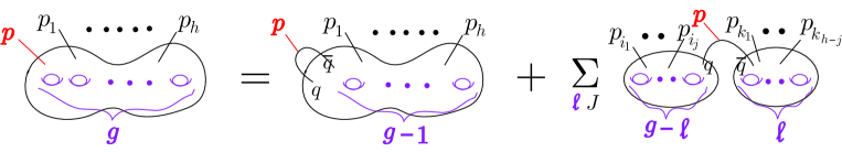
Figure 2: Structure of the Eynard-Orantin topological recursion relation (3.2)

In the following we consider the case that the character variety ${\cal C}$ is a genus ${\overline{g}}$ (distinguished from the genus $g$ of the world sheet) curve with two sheets. From the one-form $\omega(p)=\log l(p)dx(p)/x(p)$, one defines $y(p)dp=(\omega(p)-\omega({\bar{p}}))/2$ as proposed in [14, 15]:

$$y(p)=M(p)\sqrt{\sigma(p)},\quad\sigma(p)=\prod_{i=1}^{2{\overline{g}}+2}(p-q_{i}),\quad M(p)=\frac{1}{p\sqrt{\sigma(p)}}\tanh^{-1}\Big{[}\frac{\sqrt{\sigma(p)}}{f(p)}\Big{]},$$ (3.5)

where $\mbox{Re}(q_{1})\leq\mbox{Re}(q_{2})\leq\ldots\leq\mbox{Re}(q_{2{\overline{g}}+2})$, $f(p)$ is a rational function in $p$, and $M(p)$ is called the moment function in the context of matrix models [47, 48]. In this case in [49] it is found that the third type differential $dE_{q,\bar{q}}(p)$ has the form:

$$dE_{q,\bar{q}}(p)=-\frac{\sqrt{\sigma(q)}}{2\sqrt{\sigma(p)}}\Big{(}\frac{1}{p-q}-\sum_{i=1}^{{\overline{g}}}C_{i}(q)L_{i}(p)\Big{)}dp,\quad C_{i}(q)=\frac{1}{2\pi i}\oint_{q\not\in A_{i}}\frac{dp}{(p-q)\sqrt{\sigma(p)}},$$ (3.6)

where we introduced the (normalized) basis of the holomorphic differentials $L_{i}(p)dp/\sqrt{\sigma(p)}$ on ${\cal C}$ by

$$\oint_{A_{j}}\frac{L_{i}(q)}{\sqrt{\sigma(q)}}dq=2\pi i\delta_{i,j},\quad L_{i}(q)=\sum_{j=1}^{{\overline{g}}}L_{j,i}q^{j-1},\quad i=1,\ldots,{\overline{g}}.$$ (3.7)

Note that when $q$ approaches a branch point $q_{i}$, (3.6) cannot be used, i.e. if a contour $A_{i}$ contains the point $q$, instead one must replace $C_{j}(q)$ with $C_{j}(q)+\delta_{j,i}/\sqrt{\sigma(q)}$. Using the relation

$$B(p,q)=dq\frac{\partial}{\partial q}\Big{(}\frac{dp}{2(p-q)}-dE_{q,\bar{q}}(p)\Big{)},$$ (3.8)

between the Bergman kernel $B(p,q)$ and the third type differential $dE_{q,\bar{q}}(p)$, one finds that the Bergman kernel has the form:

$$B(p,q)=\frac{dpdq}{\sqrt{\sigma(p)\sigma(q)}}\Big{(}\frac{\sqrt{\sigma(p)\sigma(q)}+F(p,q)}{2(p-q)^{2}}+\frac{H(p,q)}{4}\Big{)},$$ (3.10)

$$F(p,q):=\frac{1}{2}\bigl{(}\sigma(p)+\sigma(q)\bigr{)}-\frac{p-q}{4}\bigl{(}\partial_{p}\sigma(p)-\partial_{q}\sigma(q)\bigr{)},$$

where $H(p,q)$ is a symmetric polynomial in $p$ and $q$ [49].

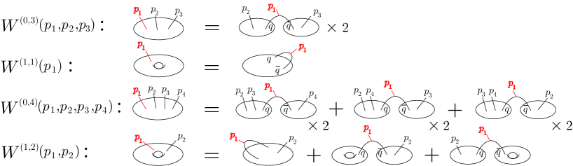
Figure 3: Diagrammatic representation of (3.11), (3.1), (LABEL:eqn:3.13), and (3.14)

Let us compute the multilinear meromorphic differentials $\widetilde{W}^{(g,h)}(p_{1},\ldots,p_{h})$ up to the Euler number $\chi=-2$ using the topological recursion relation (3.2):

$$W^{(0,3)}(p_{1},p_{2},p_{3})=\sum_{q_{i}\in{\cal C}}\mathop{\mbox{Res}}_{q=q_{i}}\frac{2dE_{q,\bar{q}}(p_{1})}{\omega(q)-\omega(\bar{q})}B(p_{2},q)B(p_{3},{\bar{q}}),$$ (3.11)

$$W^{(1,1)}(p_{1})=\sum_{q_{i}\in{\cal C}}\mathop{\mbox{Res}}_{q=q_{i}}\frac{dE_{q,\bar{q}}(p_{1})}{\omega(q)-\omega(\bar{q})}B(q,{\bar{q}}),$$

$$W^{(0,4)}(p_{1},p_{2},p_{3},p_{4})=\sum_{q_{i}\in{\cal C}}\mathop{\mbox{Res}}_{q=q_{i}}\frac{2dE_{q,\bar{q}}(p_{1})}{\omega(q)-\omega(\bar{q})}\left\{B(p_{2},\bar{q})W^{(0,3)}(p_{3},p_{4},q)+\mbox{perm}(p_{2},p_{3},p_{4})\right\},$$

$$W^{(1,2)}(p_{1},p_{2})=\sum_{q_{i}\in{\cal C}}\mathop{\mbox{Res}}_{q=q_{i}}\frac{dE_{q,\bar{q}}(p_{1})}{\omega(q)-\omega(\bar{q})}\left\{W^{(0,3)}(p_{2},q,\bar{q})+2W^{(1,1)}(q)B(p_{2},{\bar{q}})\right\},$$ (3.14)

where these differentials are represented in Fig.3. One can expand these differentials by the kernel differentials [15],

$$\chi_{i}^{(n)}(p): = \mathop{\mbox{Res}}_{q=q_{i}}\Big{(}-\frac{dE_{q,\bar{q}}(p)}{y(q)}\frac{1}{(q-q_{i})^{n}}\Big{)}$$ (3.15)

$$= \frac{dp}{2(n-1)!\sqrt{\sigma(p)}}\frac{\partial^{n-1}}{\partial q^{n-1}}\Big{\arrowvert}_{q=q_{i}}\frac{1}{M(q)}\Big{(}\frac{1}{p-q}-\sum_{i=1}^{{\overline{g}}}C_{i}(q)L_{i}(p)\Big{)},$$

where in the second equality (3.6) is utilized. Using the relation (3.8), one can expand $B(p,q)$ around $s^{2}=q-q_{i}=0$ as

$$B(p,q)\simeq M_{i}\sqrt{\sigma_{i}^{\prime}}ds\Bigl{\{}\chi_{i}^{(1)}(p)+3s^{2}\Bigl{(}\chi_{i}^{(2)}(p)+\Bigl{(}\frac{M_{i}^{\prime}}{M_{i}}+\frac{\sigma_{i}^{\prime\prime}}{4\sigma_{i}^{\prime}}\Bigr{)}\chi_{i}^{(1)}(p)\Bigr{)}$$

$$+5s^{4}\Bigl{(}\chi_{i}^{(3)}(p)+\Bigl{(}\frac{M_{i}^{\prime}}{M_{i}}+\frac{\sigma_{i}^{\prime\prime}}{4\sigma_{i}^{\prime}}\Bigr{)}\chi_{i}^{(2)}(p)+\frac{1}{2}\Bigl{(}\frac{M_{i}^{\prime\prime}}{M_{i}}+\frac{M_{i}^{\prime}\sigma_{i}^{\prime\prime}}{2M_{i}\sigma_{i}^{\prime}}+\frac{\sigma_{i}^{\prime\prime\prime}}{6\sigma_{i}^{\prime}}-\frac{\sigma_{i}^{\prime\prime 2}}{16\sigma_{i}^{\prime 2}}\Bigr{)}\chi_{i}^{(1)}(p)\Bigr{)}+{\cal{O}}(s^{6})\Bigr{\}},$$

(3.16)

where $M_{i}:=M(q_{i}),~{}\sigma_{i}^{\prime}:=\sigma^{\prime}(q_{i})$ etc., and the odd terms in $s$ are ignored because these terms are irrelevant in the computation of the topological recursion (3.2). Therefore from (3.11) one obtains [15],

$$W^{(0,3)}(p_{1},p_{2},p_{3})=\frac{1}{2}\sum_{i}M_{i}^{2}\sigma_{i}^{\prime}\chi_{i}^{(1)}(p_{1})\chi_{i}^{(1)}(p_{2})\chi_{i}^{(1)}(p_{3}).$$ (3.17)

When $q={\bar{p}}$ the Bergman kernel (3.10) yields

$$B(p,{\bar{p}})=\lim_{q\to p}\frac{dpdp}{2(p-q)^{2}}\Big{(}1-\frac{F(p,q)}{\sqrt{\sigma(p)\sigma(q)}}\Big{)}-\frac{H(p)dpdp}{4\sigma(p)}=\frac{dpdp}{4}\Big{(}\frac{\sigma^{\prime\prime}(p)}{2\sigma(p)}-\frac{\sigma^{\prime}(p)^{2}}{4\sigma(p)^{2}}-\frac{H(p)}{\sigma(p)}\Big{)},$$ (3.18)

where $H(p):=H(p,p)$, and then this can be expanded around a branch point $p=q_{i}$ as:

$$B(p,{\bar{p}})\simeq-\frac{dpdp}{4(p-q_{i})}\Big{\{}\frac{1}{4(p-q_{i})}+\Big{(}\frac{H(q_{i})}{\sigma^{\prime}(q_{i})}-\frac{\sigma^{\prime\prime}(q_{i})}{4\sigma^{\prime}(q_{i})}\Big{)}+{\cal O}(p-q_{i})\Big{\}}.$$ (3.19)

Using this expansion, from (3.1) one finds [15]:

$$W^{(1,1)}(p_{1})=\frac{1}{16}\sum_{i}\chi_{i}^{(2)}(p_{1})+\frac{1}{4}\sum_{i}\Big{(}\frac{H(q_{i})}{\sigma_{i}^{\prime}}-\frac{\sigma_{i}^{\prime\prime}}{4\sigma_{i}^{\prime}}\Big{)}\chi_{i}^{(1)}(p_{1}).$$ (3.20)

To compute (LABEL:eqn:3.13) and (3.14) let us write the kernel differentials in terms of the polynomials $F(p,q)$ and $H(p,q)$ by comparing the expansion (3.16) with the expansion of (3.10) around $s^{2}=q-q_{i}=0$,

$$B(p,q) = \frac{dpdq}{4s\sqrt{\sigma(p)}}V(p,q;q_{i}),\quad V(p,q;q_{i}):=\frac{1}{\sqrt{\sigma(q;q_{i})}}\Bigl{(}H(p,q)+\frac{2F(p,q)}{(p-q)^{2}}\Bigr{)},\hskip 16.00008pt$$ (3.21)

$$\simeq \frac{dpdq}{4s\sqrt{\sigma(p)}}\Big{\{}V(p,q_{i};q_{i})+s^{2}\partial_{q}V(p,q_{i};q_{i})+\frac{s^{4}}{2}\partial_{q}^{2}V(p,q_{i};q_{i})+{\cal{O}}(s^{6})\Big{\}},$$

where $\sigma(q;q_{i}):=\sigma(q)/(q-q_{i})$, and we have removed the term $dpdq/2(p-q)^{2}$ in the expansion which is irrelevant in the computation of the topological recursion (3.2). Some of the kernel differentials are

$$\chi_{i}^{(1)}(p) = \frac{dp}{2M_{i}\sigma_{i}^{\prime}\sqrt{\sigma(p)}}{\widetilde{V}}(p,q_{i}),\quad{\widetilde{V}}(p,q):=H(p,q)+\frac{2F(p,q)}{(p-q)^{2}},$$ (3.22)

$$\chi_{i}^{(2)}(p) = \frac{dp}{6M_{i}\sigma_{i}^{\prime}\sqrt{\sigma(p)}}\partial_{q}{\widetilde{V}}(p,q_{i})-\Big{(}\frac{M_{i}^{\prime}}{M_{i}}+\frac{\sigma_{i}^{\prime\prime}}{3\sigma_{i}^{\prime}}\Big{)}\chi_{i}^{(1)}(p),$$ (3.23)

$$\chi_{i}^{(3)}(p) = \frac{dp}{20M_{i}\sigma_{i}^{\prime}\sqrt{\sigma(p)}}\partial_{q}^{2}{\widetilde{V}}(p,q_{i})$$

$$-\Big{(}\frac{M_{i}^{\prime\prime}}{2M_{i}}+\frac{2M_{i}^{\prime}\sigma_{i}^{\prime\prime}}{5M_{i}\sigma_{i}^{\prime}}+\frac{\sigma_{i}^{\prime\prime\prime}}{10\sigma_{i}^{\prime}}\Big{)}\chi_{i}^{(1)}(p)-\Big{(}\frac{M_{i}^{\prime}}{M_{i}}+\frac{2\sigma_{i}^{\prime\prime}}{5\sigma_{i}^{\prime}}\Big{)}\chi_{i}^{(2)}(p).$$ (3.24)

In the following for simplicity we only discuss the cases of ${\overline{g}}=1$. In this case the Bergman kernel is concretely given by the Akemann’s formula [48, 18]:

$$B(p,q)=\frac{dpdq}{\sqrt{\sigma(p)\sigma(q)}}\Big{(}\frac{\sqrt{\sigma(p)\sigma(q)}+f(p,q)}{2(p-q)^{2}}+\frac{G(k)}{4}\Big{)},$$ (3.25)

$$f(p,q):=p^{2}q^{2}-\frac{1}{2}pq(p+q)S_{1}+\frac{1}{6}(p^{2}+4pq+q^{2})S_{2}-\frac{1}{2}(p+q)S_{3}+S_{4},$$ (3.26)

$$G(k):=-\frac{1}{3}S_{2}+(q_{1}q_{2}+q_{3}q_{4})-\frac{E(k)}{K(k)}(q_{1}-q_{3})(q_{2}-q_{4}),$$ (3.28)

$$K(k)=\int_{0}^{1}\frac{dt}{\sqrt{(1-t^{2})(1-k^{2}t^{2})}},~{}E(k)=\int_{0}^{1}dt\sqrt{\frac{1-k^{2}t^{2}}{1-t^{2}}},$$

where $K(k)$, (resp. $E(k)$) is the complete elliptic integral of the first, (resp. second) kind with the modulus $k^{2}=\frac{(q_{1}-q_{2})(q_{3}-q_{4})}{(q_{1}-q_{3})(q_{2}-q_{4})}$, and $S_{k}=\sum_{1\leq j_{1}<j_{2}<\ldots<j_{k}\leq 4}q_{j_{1}}q_{j_{2}}\cdots q_{j_{k}}$, $k=1,\ldots,4$ are the elementary symmetric polynomials of the branch points $q_{i}$. By comparing (3.10) with (3.25), we see that ${\widetilde{V}}(p,q)$ in the kernel differentials is given by

$${\widetilde{V}}(p,q)=G(k)+\frac{2f(p,q)}{(p-q)^{2}}.$$ (3.29)

After some computation, (LABEL:eqn:3.13) and (3.14) are expanded by the kernel differentials (see appendix B for the detailed derivation), and we summarize the results as follows:

$$W^{(0,3)}(p_{1},p_{2},p_{3})=\frac{1}{2}\sum_{i}M_{i}^{2}\sigma_{i}^{\prime}\chi_{i}^{(1)}(p_{1})\chi_{i}^{(1)}(p_{2})\chi_{i}^{(1)}(p_{3}),$$ (3.30)

$$W^{(1,1)}(p_{1})=\frac{1}{16}\sum_{i}\chi_{i}^{(2)}(p_{1})+\frac{1}{4}\sum_{i}\Big{(}\frac{G}{\sigma_{i}^{\prime}}-\frac{\sigma_{i}^{\prime\prime}}{12\sigma_{i}^{\prime}}\Big{)}\chi_{i}^{(1)}(p_{1}),$$

$$W^{(0,4)}(p_{1},p_{2},p_{3},p_{4})=\frac{1}{4}\sum_{i}\Big{\{}3M_{i}^{2}\Bigl{(}G+\frac{2}{3}\sigma_{i}^{\prime\prime}+3\sigma_{i}^{\prime}\frac{M_{i}^{\prime}}{M_{i}}\Bigr{)}\chi_{i}^{(1)}(p_{1})\chi_{i}^{(1)}(p_{2})\chi_{i}^{(1)}(p_{3})\chi_{i}^{(1)}(p_{4})$$

$$\quad~{}+\sum_{j\neq i}M_{i}M_{j}\Bigl{(}G+\frac{2f(q_{i},q_{j})}{(q_{i}-q_{j})^{2}}\Bigr{)}\Bigl{(}\chi_{i}^{(1)}(p_{1})\chi_{i}^{(1)}(p_{2})\chi_{j}^{(1)}(p_{3})\chi_{j}^{(1)}(p_{4})+\mbox{perm}(p_{2},p_{3},p_{4})\Bigr{)}$$

$$\quad~{}+3M_{i}^{2}\sigma_{i}^{\prime}\Bigl{(}\chi_{i}^{(1)}(p_{1})\chi_{i}^{(1)}(p_{2})\chi_{i}^{(1)}(p_{3})\chi_{i}^{(2)}(p_{4})+\mbox{perm}(p_{1},p_{2},p_{3},p_{4})\Bigr{)}\Big{\}},$$ (3.33)

$$W^{(1,2)}(p_{1},p_{2})$$

$$\quad~{}=\frac{1}{32}\sum_{i}\Big{\{}\Big{\{}\frac{8G^{2}}{\sigma_{i}^{\prime 2}}-\Bigl{(}\frac{2\sigma_{i}^{\prime\prime}}{3\sigma_{i}^{\prime 2}}-\frac{11M_{i}^{\prime}}{\sigma_{i}^{\prime}M_{i}}\Bigr{)}G-\frac{\sigma_{i}^{\prime\prime 2}}{12\sigma_{i}^{\prime 2}}-\frac{5\sigma_{i}^{\prime\prime\prime}}{18\sigma_{i}^{\prime}}-\frac{7\sigma_{i}^{\prime\prime}M_{i}^{\prime}}{6\sigma_{i}^{\prime}M_{i}}+\frac{5M_{i}^{\prime\prime}}{2M_{i}}-\frac{3M_{i}^{\prime 2}}{M_{i}^{2}}$$

$$\quad~{}+\sum_{j\neq i}\frac{M_{i}}{M_{j}\sigma_{j}^{\prime 2}}\Big{[}\Bigl{(}4G-\frac{2}{3}\sigma_{j}^{\prime\prime}-\sigma_{j}^{\prime}\frac{M_{j}^{\prime}}{M_{j}}\Bigr{)}\Bigl{(}G+\frac{2f(q_{i},q_{j})}{(q_{i}-q_{j})^{2}}\Bigr{)}-\frac{\sigma_{i}^{\prime}\sigma_{j}^{\prime}}{3(q_{i}-q_{j})^{2}}\Big{]}\Big{\}}\chi_{i}^{(1)}(p_{1})\chi_{i}^{(1)}(p_{2})$$

$$\quad~{}+\sum_{j\neq i}\frac{4}{\sigma_{i}^{\prime}\sigma_{j}^{\prime}}\Big{(}G+\frac{2f(q_{i},q_{j})}{(q_{i}-q_{j})^{2}}\Big{)}^{2}\chi_{i}^{(1)}(p_{1})\chi_{j}^{(1)}(p_{2})+5\Big{(}\chi_{i}^{(1)}(p_{1})\chi_{i}^{(3)}(p_{2})+(p_{1}\leftrightarrow p_{2})\Big{)}$$

$$\quad~{}+\Bigl{(}\frac{12G}{\sigma_{i}^{\prime}}-\frac{\sigma_{i}^{\prime\prime}}{2\sigma_{i}^{\prime}}+\frac{2M_{i}^{\prime}}{M_{i}}\Bigr{)}\left(\chi_{i}^{(1)}(p_{1})\chi_{i}^{(2)}(p_{2})+(p_{1}\leftrightarrow p_{2})\right)+3\chi_{i}^{(2)}(p_{1})\chi_{i}^{(2)}(p_{2})\Big{\}}.$$

In the following, we define free energies on character variety, and compute them using the above results for two concrete examples described in section 2.2 and 2.3 where the character varieties are reduced to genus one curve with two sheets on the geometric branch.

3.2 Free energy on character variety

Let us concentrate on the genus one case in (3.5):

$$y(p)=M(p)\sqrt{\sigma(p)},\quad\sigma(p)=\prod_{i=1}^{4}(p-q_{i})=p^{4}-S_{1}p^{3}+S_{2}p^{2}-S_{3}p+S_{4},$$

$$M(p)=\frac{1}{p\sqrt{\sigma(p)}}\tanh^{-1}\Big{[}\frac{\sqrt{\sigma(p)}}{f(p)}\Big{]}=\frac{1}{2p\sqrt{\sigma(p)}}\log\frac{f(p)+\sqrt{\sigma(p)}}{f(p)-\sqrt{\sigma(p)}}.$$ (3.34)

In the following by taking the reciprocality of the A-polynomial into consideration, we assume that

$$S_{1}=S_{3},\quad S_{4}=1,\quad q_{2}=q_{1}^{-1},\quad q_{4}=q_{3}^{-1}.$$ (3.35)

The free energy $\widetilde{\cal F}^{(g,h)}(p_{1},\ldots,p_{h})$ is defined by [14, 15]:

$$\widetilde{\cal F}^{(g,h)}(p_{1},\ldots,p_{h})=\int^{p_{1}}\cdots\int^{p_{h}}W^{(g,h)}(p_{1},\ldots,p_{h}).$$ (3.36)

This free energy is related to the open topological string amplitude $F(V)$ in the A-model on the local toric Calabi-Yau 3-fold $X$ whose mirror curve is the spectral curve in the Eynard-Orantin topological recursion relation [14]:

$$F(V)=\log Z(V),\quad Z(V)=\frac{1}{Z_{\rm closed}(X)}\sum_{R}Z_{R}(X){\rm Tr}_{R}V,$$ (3.37)

$$V={\rm diag}(\xi_{1},\xi_{2},\ldots,\xi_{n}),$$ (3.38)

where $\xi_{i}$ ($i=1,\ldots,n$) denotes the location of the D-branes in the toric Calabi-Yau 3-fold $X$.

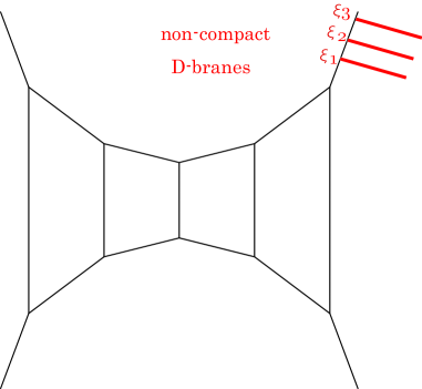
Figure 4: Toric branes inserted on the local Calabi-Yau $3$-fold

$Z_{R}(X)$ is the topological vertex amplitude on $X$ where the representation $R$ is assigned to the external leg that the D-brane is inserted.

The functional $F(V)$ is expanded as follows:

$$F(V) = \sum_{g=0}^{\infty}\sum_{h=1}^{\infty}\sum_{w_{1},\ldots,w_{h}}\frac{1}{h!}g_{s}^{2g-2+h}F_{\{w\},g}{\rm Tr}V^{w_{1}}\cdots{\rm Tr}V^{w_{h}}.$$ (3.39)

After identifying

$${\rm Tr}V^{w_{1}}\cdots{\rm Tr}V^{w_{h}}\quad\longleftrightarrow\quad p_{1}^{w_{1}}\cdots p_{h}^{w_{h}},$$ (3.40)

the functional $F(V)$ is related to the free energy $\widetilde{\cal F}^{(g,h)}$:

$$F(V)\quad\longleftrightarrow\quad\sum_{g=0}^{\infty}\sum_{h=1}^{\infty}g_{s}^{2g-2+h}\widetilde{\cal F}^{(g,h)}(p_{1},\ldots,p_{h}).$$ (3.41)

As an assumption of our proposal, we introduce the D-branes whose locations are specified formally by

$$V=\left(\begin{array}[]{cc}p&0\\ 0&p^{-1}\end{array}\right).$$ (3.44)

This choice of $V$ is nothing but the $PSL(2;\mathbb{C})$ holonomy representation matrix $\rho(\mu)$ along the meridian cycle $\mu$, and this free energy respects the reciprocality of the character variety as was considered in [8]. Actually we see that the free energy ${\cal F}(p)$ is obtained from the free energy $\widetilde{\cal F}(p)$ for one brane at a point $p$ by ${\cal F}(p)=\widetilde{\cal F}(p+p^{-1})$. Because the multilinear meromorphic differentials $W^{(g,h)}(p_{1},\ldots,p_{h})$ can be expanded in terms of the kernel differentials (3.15) as in (3.30) - (3.33), it is convenient to introduce averaged kernel differentials:

$$\widetilde{\chi}_{i}^{(n)}(p): = \chi_{i}^{(n)}(p)+\chi_{i}^{(n)}(p^{-1})=\frac{dp}{2(n-1)!\sqrt{\sigma(p)}}\frac{\partial^{n-1}}{\partial q^{n-1}}\Big{\arrowvert}_{q=q_{i}}\frac{1}{M(q)}\Big{(}\frac{1}{p-q}-\frac{1}{p^{-1}-q}\Big{)}$$ (3.45)

$$= \frac{dw}{2(n-1)!\sqrt{\widetilde{\sigma}(w)}}\frac{\partial^{n-1}}{\partial q^{n-1}}\Big{\arrowvert}_{q=q_{i}}\frac{1}{qM(q)}\frac{1}{w-\alpha},$$

where $w=(p+p^{-1})/2$, $\alpha=(q+q^{-1})/2$. We have defined

$$\widetilde{\sigma}(w):=\frac{\sigma(p)}{p^{2}}=4w^{2}-2S_{1}w+(S_{2}-2)=4(w-\alpha_{1})(w-\alpha_{2}),$$ (3.46)

where $\alpha_{1}=(q_{1}+q_{1}^{-1})/2=(q_{2}+q_{2}^{-1})/2$ and $\alpha_{2}=(q_{3}+q_{3}^{-1})/2=(q_{4}+q_{4}^{-1})/2$. Using (3.45) by replacing $\chi_{i}^{(n)}(p)$ with $\widetilde{\chi}_{i}^{(n)}(p)$, we define averaged multilinear meromorphic differentials $\widetilde{W}^{(g,h)}(p_{1},\ldots,p_{h})$ for $(g,h)\neq(0,1),(0,2)$, and define free energies ${\cal F}^{(g,h)}(p)$ (according to remodeling the B-model [14, 15]) for the two toric branes on the character variety ${\cal C}$ as:

$${\cal F}^{(g,h)}(p):=\frac{1}{h!}{\cal F}^{(g,h)}(p,\ldots,p),$$ (3.47)

$${\cal F}^{(g,h)}(p_{1},\ldots,p_{h}):=\int^{p_{1}}\int^{p_{2}}\cdots\int^{p_{h}}{\overline{W}}^{(g,h)}(p_{1}^{\prime},\ldots,p_{h}^{\prime}),$$ (3.48)

$${\overline{W}}^{(0,1)}(p):=\omega(p)+\omega(p^{-1}):=\log l(p)\frac{dp}{p}+\log l(p^{-1})\frac{dp^{-1}}{p^{-1}},$$ (3.49)

$${\overline{W}}^{(0,2)}(p_{1},p_{2}):=2B(p_{1},p_{2})+2B(p_{1},p_{2}^{-1})-\frac{2dw_{1}dw_{2}}{(w_{1}-w_{2})^{2}},\quad w_{i}=\frac{p_{i}+p_{i}^{-1}}{2},$$ (3.50)

$${\overline{W}}^{(g,h)}(p_{1},\ldots,p_{h}):=\widetilde{W}^{(g,h)}(p_{1},\ldots,p_{h})~{}\mbox{for}~{}(g,h)\neq(0,1),(0,2),$$ (3.51)

where the factor $h!$ in (3.47) is the symmetric factor. In (3.50) the factor $2$ comes from $B(p^{-1}_{1},p^{-1}_{2})+B(p^{-1}_{1},p_{2})$ where $B(p_{1},p_{2})=B(p^{-1}_{1},p^{-1}_{2})$, and the term $dw_{1}dw_{2}/(w_{1}-w_{2})^{2}$ needs for the regularization (exclusion of the double pole) of the Bergman kernel at $p_{1}=p_{2}$. By introducing a coupling constant $g_{s}$, we define

$${\cal F}(p):=\frac{1}{2}\sum_{g=0,h=1}^{\infty}g_{s}^{2g-2+h}{\cal F}^{(g,h)}(p)=\sum_{n=0}^{\infty}{\tilde{\hbar}}^{n-1}{\cal F}_{n}(p)$$ (3.52)

on the character variety ${\cal C}$, where to express “chiral part” of the free energy we insist the necessity of the factor $1/2$. We also introduced a new coupling constant ${\tilde{\hbar}}=g_{s}/2$ for a consistency with the coupling constant $\hbar$ in the Chern-Simons gauge theory.

Note that in the definition (3.48), there are ambiguities of the integration constants. In this paper we claim that, by taking the universal part which does not depend on the choice of the integration constants, we obtain

$${\cal F}_{n}(p)\simeq S_{n}^{({\rm geom})}(u),\quad p=m^{2}=e^{2u}.$$ (3.53)

Here $S_{n}^{({\rm geom})}(u)$ is the perturbative invariant on the geometric branch discussed in section 2. In this claim we neglect the constant term in $S_{n}^{({\rm geom})}(u)$ which does not depend on $u$. In the left hand side of the above claim, regularizations of $G(k)^{n}$ in (3.28), as explained in the following, are needed.

In the rest of this section, to check this claim we compute

$${\cal F}_{2}(p)={\cal F}^{(0,3)}(p)+{\cal F}^{(1,1)}(p),$$ (3.54)

$${\cal F}_{3}(p)=2{\cal F}^{(0,4)}(p)+2{\cal F}^{(1,2)}(p),$$ (3.55)

for the two examples of section 2.2 and 2.3, and find that the different regularizations for $G(k)$ in the Bergman Kernel (3.25), and its square $G(k)^{2}$ are needed as:

$$G(k)=-\frac{1}{3}S_{2}+2-\frac{E(k)}{K(k)}(q_{1}-q_{3})(q_{2}-q_{4})~{}\Rightarrow~{}G_{1}:=-\frac{1}{3}S_{2}+2,\hskip 50.00008pt$$ (3.56)

$$G(k)^{2}~{}\Rightarrow~{}G_{2}:=G_{1}^{2}-(1-k^{2})(q_{1}-q_{3})^{2}(q_{2}-q_{4})^{2}=G_{1}^{2}-\big{(}S_{1}^{2}-4(S_{2}-2)\big{)},$$ (3.57)

for the examples, where $k$ is the modulus of the elliptic integrals $K(k)$ and $E(k)$ defined in (3.28). The constant $G$ is determined uniquely by imposing zero A-period condition. But we have to impose some ad-hoc regularizations to $G^{n}$ terms in the free energy. This regularization may be compensating the some subtleties of the correspondence in the higher order terms of $\hbar$ expansion. The subtleties may come from the choice of the integration contour for the BKMP’s free energy or ${\cal O}(\hbar/2)$ shift of the moduli of the A-polynomial. Although we do not know the general rule for this regularizations, we heuristically find the rules which are applicable to some lower order terms in the WKB expansion. In appendix D we compute the free energy ${\cal F}_{4}(p)$, and for the figure eight knot complement we find that different regularizations for $G(k)$ in ${\cal F}^{(1,3)}(p)$ and in ${\cal F}^{(2,1)}(p)$ are needed as in (D.10).

The leading term in the correspondence (3.53) is understood as follows. By the reciprocality of the A-polynomial, the character variety has the property $l(p)l(p^{-1})=1$. Therefore we obtain

$${\cal F}_{0}(p)=\frac{1}{4}{\cal F}^{(0,1)}(p)=\frac{1}{2}\int^{p}\log l(p)\frac{dp}{p}=\int^{m}\log l(m)\frac{dm}{m},$$ (3.58)

and this is nothing but $S_{0}^{({\rm geom})}(u)$, where $p=m^{2}$, except a constant shift [39, 50]. The subleading term ${\cal F}_{1}(p)={\cal F}^{(0,2)}(p)/2$ is discussed in [8] (see also appendix C). In the rest of this section we check the above claim for two concrete examples in section 2.

3.3 Figure eight knot complement

As the first example, from the A-polynomial (2.32) of the figure eight knot, we obtain the data of the curve:

$$\sigma(p)=p^{4}-2p^{3}-p^{2}-2p+1,\quad\widetilde{\sigma}(w)=4w^{2}-4w-3,$$ (3.59)

$$f(p)=\frac{p^{4}-p^{3}-2p^{2}-p+1}{p^{2}-1},$$ (3.60)

where $w=(p+p^{-1})/2$, and $\widetilde{\sigma}(w)=\sigma(p)/p^{2}$.

The free energy ${\cal F}_{2}(p)$ defined in (3.54) is computed from (3.30) and (3.1):

$$\frac{\overline{W}^{(0,3)}(p_{1},p_{2},p_{3})}{dw_{1}dw_{2}dw_{3}}=\frac{8\big{[}(2w_{1}-3)(2w_{2}-3)(2w_{3}-3)+(2w_{1}+1)(2w_{2}+1)(2w_{3}+1)\big{]}}{\widetilde{\sigma}(w_{1})^{3/2}\widetilde{\sigma}(w_{2})^{3/2}\widetilde{\sigma}(w_{3})^{3/2}},$$

$$\frac{\overline{W}^{(1,1)}(p)}{dw}=\frac{-(2w-3)^{2}+(2w+1)^{2}}{4\widetilde{\sigma}(w)^{5/2}}+\frac{-5(3G+2)(2w-3)+3(3G-2)(2w+1)}{180\widetilde{\sigma}(w)^{3/2}}.$$

(3.62)

Thus from (3.47) and (3.54) we obtain

$${\cal F}^{(0,3)}(p)=-\frac{12w^{2}-12w+7}{12\widetilde{\sigma}(w)^{3/2}},$$ (3.63)

$${\cal F}^{(1,1)}(p)=-\frac{1}{3\widetilde{\sigma}(w)^{3/2}}-\frac{2(6G+1)w-9(G+1)}{180\widetilde{\sigma}(w)^{1/2}},$$ (3.64)

$${\cal F}_{2}(p)=-\frac{1}{12\widetilde{\sigma}(w)^{3/2}}\Big{\{}\frac{8(6G+1)}{15}w^{3}-\frac{4(21G-34)}{15}w^{2}-10w+\frac{9G+64}{5}\Big{\}}.$$ (3.65)

Using the regularization (3.56), by replacing $G$ with $G_{1}=7/3$ we get

$${\cal F}_{2}(p)=-\frac{1}{12\widetilde{\sigma}(w)^{3/2}}(8w^{3}-4w^{2}-10w+17).$$ (3.66)

This coincides with the perturbative invariant (2.36) by identifying the parameter $w=(m^{2}+m^{-2})/2$.

Next from (3.33) and (3.33) we compute the free energy ${\cal F}_{3}(p)$ defined in (3.55). As the result by (3.47) and (3.55) we obtain

$${\cal F}^{(0,4)}(p)=\frac{1}{\widetilde{\sigma}(w)^{3}}\Big{(}\frac{4}{3}w^{5}-\frac{8}{3}w^{4}+2w^{3}+\frac{11}{3}w^{2}-\frac{67}{12}w+\frac{25}{12}\Big{)},\hskip 75.0001pt$$ (3.67)

$${\cal F}^{(1,2)}(p)=\frac{1}{\widetilde{\sigma}(w)^{3}}\Big{(}\frac{16}{81}w^{6}-\frac{568}{405}w^{5}+\frac{821}{405}w^{4}+\frac{154}{45}w^{3}-\frac{83}{30}w^{2}-\frac{61}{15}w+\frac{859}{240}\Big{)}$$ (3.68)

$$\hskip 50.00008pt+\frac{G}{\widetilde{\sigma}(w)^{2}}\Big{(}\frac{8}{135}w^{4}-\frac{29}{135}w^{3}+\frac{13}{90}w^{2}+\frac{7}{20}w-\frac{9}{40}\Big{)}+\frac{G^{2}(4w-3)^{2}}{3600\widetilde{\sigma}(w)},$$

$${\cal F}_{3}(p)=\frac{2}{\widetilde{\sigma}(w)^{3}}\Big{(}\frac{16}{81}w^{6}-\frac{28}{405}w^{5}-\frac{259}{405}w^{4}+\frac{244}{45}w^{3}+\frac{9}{10}w^{2}-\frac{193}{20}w+\frac{453}{80}\Big{)}$$ (3.69)

$$\hskip 50.00008pt+\frac{2G}{\widetilde{\sigma}(w)^{2}}\Big{(}\frac{8}{135}w^{4}-\frac{29}{135}w^{3}+\frac{13}{90}w^{2}+\frac{7}{20}w-\frac{9}{40}\Big{)}+\frac{G^{2}(4w-3)^{2}}{1800\widetilde{\sigma}(w)},$$

and using the regularization (3.56) and (3.57), by replacing $G$ with $G_{1}=7/3$ and $G^{2}$ with $G_{2}=-95/9$ we get

$${\cal F}_{3}(p)=\frac{2}{\widetilde{\sigma}(w)^{3}}(8w^{3}-4w^{2}-10w+7).$$ (3.70)

This also coincides with the perturbative invariant (2.37).

3.4 Once punctured torus bundle over $\mathbb{S}^{1}$ with holonomy $L^{2}R$

As the second example, from the A-polynomial (2.55) of the once punctured torus bundle over $\mathbb{S}^{1}$ with holonomy $L^{2}R$, we obtain the data of the curve:

$$\sigma(p)=p^{4}-2p^{3}-5p^{2}-2p+1,\quad\widetilde{\sigma}(w)=4w^{2}-4w-7,$$ (3.71)

$$f(p)=\frac{p^{3}-2p^{2}-2p+1}{p-1},$$ (3.72)

where $\widetilde{\sigma}(w)=\sigma(p)/p^{2}$.

As same as the computation in section 3.3, the free energies ${\cal F}^{(0,3)}(p)$ and ${\cal F}^{(1,1)}(p)$ are obtained as:

$${\cal F}^{(0,3)}(p)=-\frac{8w^{3}+36w^{2}+6w+19}{48\widetilde{\sigma}(w)^{3/2}},\hskip 180.00027pt$$ (3.73)

$${\cal F}^{(1,1)}(p)=-\frac{(72G-40)w^{3}-(156G-12)w^{2}-(42G-210)w+147G+217}{336\widetilde{\sigma}(w)^{3/2}},$$ (3.74)

and using the regularization (3.56), by replacing $G$ with $G_{1}=11/3$ we find

$${\cal F}_{2}(p)=-\frac{1}{48\widetilde{\sigma}(w)^{3/2}}(40w^{3}-44w^{2}+14w+127).$$ (3.75)

This coincides with the perturbative invariant (2.62) by identifying the parameter $w=(m^{2}+m^{-2})/2$.

The free energies ${\cal F}^{(0,4)}(p)$ and ${\cal F}^{(1,2)}(p)$ are also computed. Using the regularization (3.56) and (3.57), by replacing $G$ with $G_{1}=11/3$ and $G^{2}$ with $G_{2}=-167/9$ we find

$${\cal F}_{3}(p)=-\frac{1}{128\widetilde{\sigma}(w)^{3}}(64w^{6}-192w^{5}-1168w^{4}-3488w^{3}+2300w^{2}+2996w-2071).$$ (3.76)

For the free energy ${\cal F}_{3}(p)$ we should consider an imaginary term corresponding to the Chern-Simons term of the partition function for the state integral model as in (2.62). Such the contribution, if we add a constant term $1/128$:

$${\cal F}_{3}(p)+\frac{1}{128}=\frac{1}{2\widetilde{\sigma}(w)^{3}}(16w^{4}+64w^{3}-32w^{2}-56w+27),$$ (3.77)

then this coincides with the perturbative invariant (2.63).

4 Torus knots

In this section, we will further discuss the correspondence for torus knots. The perturbative invariants $S_{k}(u)$ and the BKMP’s free energies ${\cal F}_{k}$ are computed exactly for this case. Although the results are rather trivial on both sides, we are able to check the correspondence exactly for this example.

4.1 Colored Jones polynomial for torus knots

A torus knot is described as a curve on a two-torus $\mathbb{T}^{2}$, and a pair of coprime integers $(p,q)$ specifies the number of windings around each cycle of $\mathbb{T}^{2}$. For the $(p,q)$ torus knot the colored Jones polynomial is found explicitly [51].

Although a torus knot does not admit a hyperbolic structure on the $\mathbb{S}^{3}$ complement, the asymptotic behavior of the the colored Jones polynomials is studied in the context of the Melvin-Morton-Rozansky conjecture [52, 51, 53, 54, 55] and the volume conjecture [56, 57, 58]. In the analysis of the volume conjecture, the volume of the torus knot complement vanishes but the Chern-Simons invariant [59] is realized as the asymptotic limit of the colored Jones polynomial around the exponential growth point.

Furthermore, the $q$-difference equation for the $(p,q)$ torus knots have been found explicitly [31, 32, 33, 34, 35]. Adopting the technique of [21], we will perform the WKB expansion iteratively from the $q$-difference equation.

4.2 AJ conjecture for torus knots

The $q$-difference equations for $(2,2\mathfrak{m}+1)$ torus knots $T_{2,2\mathfrak{m}+1}$ are found from the inhomogeneous difference equation [35]:

$$J_{n}({T_{2,2\mathfrak{m}+1}};q)=q^{\mathfrak{m}(n-1)}\frac{1-q^{2n-1}}{1-q^{n}}-q^{(2\mathfrak{m}+1)n-\mathfrak{m}}\frac{1-q^{n-1}}{1-q^{n}}J_{n-1}({T_{2,2\mathfrak{m}+1}};q),$$ (4.1)

$$J_{n}({T_{s,t}};q)=\frac{q^{\frac{1}{2}(s-1)(t-1)(n-1)}}{1-q^{n}}(1-q^{s(n-1)+1}-q^{t(n-1)+1}+q^{(s+t)(n-1)})$$

$$\quad\quad\quad\quad\quad\;\;+\frac{1-q^{n-2}}{1-q^{n}}q^{st(n-1)+1}J_{n-2}(T_{s,t};q).$$ (4.2)

As was firstly calculated in [31, 32], one can obtain the homogeneous $q$-difference equation from the inhomogeneous one by adopting Mathematica packages ‘qZeil.m’ and ‘qMultiSum.m’ developed by Paule and Riese [60].

For the trefoil knot ${\bf 3_{1}}$ the $q$-difference equation for the colored Jones polynomial is [34]:

$$P_{\bf 3_{1}}(E,Q)J_{n}({\bf 3_{1}};q)=0,$$ (4.3)

$$P_{\bf 3_{1}}(E,Q)=\frac{q^{2}Q^{2}(q^{2}-q^{2}Q)}{q^{3}-q^{4}Q^{2}}$$

$$\quad\quad\quad\quad\quad\quad+\frac{(q-q^{2}Q)(q+q^{2}Q)(q^{4}-q^{5}Q+q^{6}Q^{2}-q^{7}Q^{2}-q^{7}Q^{3}+q^{8}Q^{4})}{q^{2}Q(q-q^{4}Q^{2})(q^{3}-q^{4}Q^{2})}E$$

$$\quad\quad\quad\quad\quad\quad+\frac{-1+q^{2}Q}{Q(q-q^{4}Q^{2})}E^{2},$$ (4.4)

where

$$(Qf)(n)=q^{n}f(n),\quad(Ef)(n)=f(n+1),\quad q=e^{2\hbar}.$$ (4.5)

In $\hbar\to 0$ limit, the polynomial $P_{\bf 3_{1}}$ yields

$$P_{\bf 3_{1}}(L,M)=-\frac{(L-1)(L+M^{3})}{M(1+M)}.$$ (4.6)

The numerator of $P_{\bf 3_{1}}(L,M)$ is the A-polynomial for the trefoil knot.

The expectation value of the Wilson loop operator $W_{n}(K;q)$ is different from the colored Jones polynomial $J_{n}(K;q)$ by the unknot factor $J_{n}({\rm unknot};q)$. By factoring out $q^{j/2}Q-q^{-j/2}$ in the coefficient of $E^{j}$, one obtains the $q$-difference equation for $W_{n}(K;q)$. The Wilson loop expectation value $W_{n}(K;q)$ is identified with $Z(S^{3}\backslash K;\hbar,u)$ for $q=e^{2\hbar}$ and $m=q^{n/2}$, if $K$ is the hyperbolic knot.

We rewrite the $q$-difference equation for $W_{n}({\bf 3_{1}};q)$ following the notation of [21] as $Q=\hat{m}^{2}$:

$$\sum_{j=0}^{2}a_{j}(q^{n/2};q)W_{n+j}({\bf 3_{1}};q)=0,$$ (4.7)

$$a_{0}(\hat{m},q)=\frac{q^{2}\hat{m}^{4}}{q\hat{m}^{4}-1},$$

$$a_{1}(\hat{m},q)=-\frac{q^{1/2}(1+q\hat{m}^{2})[1-q\hat{m}^{2}-(q^{3}-q^{2})\hat{m}^{4}-q^{3}\hat{m}^{6}+q^{4}\hat{m}^{8}]}{\hat{m}^{2}(1-q^{3}\hat{m}^{4})(1-q\hat{m}^{4})},$$

$$a_{2}(\hat{m},q)=\frac{1}{\hat{m}^{2}(1-q^{3}\hat{m}^{4})}.$$

Furthermore $q$-difference operator $P_{\bf 3_{1}}$ is factorized:

$$\hat{m}^{2}(1-q\hat{m}^{4})(1-q^{3}\hat{m}^{4})P_{\bf 3_{1}}(\hat{l},\hat{m})$$

$$=(1-q\hat{m}^{4})\hat{l}^{2}-q^{1/2}(1-q^{3}\hat{m}^{4}-q^{4}\hat{m}^{6}+q^{5}\hat{m}^{10})-q^{2}(1-q^{3}\hat{m}^{4})\hat{m}^{6}$$

$$=\hat{l}(1-q^{-1}\hat{m}^{4})\hat{l}-q^{1/2}(1-q^{3}\hat{m}^{4})\hat{l}+q^{3/2}\hat{l}(1-q^{-1}\hat{m}^{4})\hat{m}^{6}-q^{2}(1-q^{3}\hat{m}^{4})\hat{m}^{6}$$

$$=\bigl{[}\hat{l}(1-q^{-1}\hat{m}^{4})-q^{1/2}(1-q^{3}\hat{m}^{4})\bigr{]}(\hat{l}+q^{3/2}\hat{m}^{6}).$$ (4.8)

There are two branches for the solution of this difference equation. One branch corresponds to the solution $l=-m^{6}$ for $P_{\bf 3_{1}}(l,m^{2})=0$ in $q\to 1$ limit, and we call this the non-abelian branch. Another branch corresponds to a solution $l=1$, and we call this the abelian branch. In the following, we will discuss the non-abelian branch for the trefoil knot. The results of abelian branch and the other torus knots are summarized in appendix A.

The perturbative invariants $S_{n}^{(\alpha)}(u)$ for the branch $\alpha$ are defined as follows:

$$W_{n}(K;q)=\exp\left[\frac{1}{\hbar}S_{0}^{(\alpha)}(u)-\frac{1}{2}\delta^{(\alpha)}\log\hbar+\sum_{n=0}^{\infty}S_{n+1}^{(\alpha)}(u)\hbar^{n}\right].$$ (4.9)

In the non-abelian branch $\alpha={\rm nab}$, the leading term yields [59, 61]

$$S_{0}^{\rm(nab)}(u) = {\rm CS}({\bf 3_{1}};0)-\int_{0}^{u}du\;v_{\rm nab}(u)+\pi iu$$ (4.10)

$$= 3\log^{2}m-\frac{\pi^{2}}{12}-2\pi^{2}s,\quad s\in\mathbb{Z},$$

$$l = -m^{6}.$$ (4.11)

The perturbative invariant for this branch satisfies the $q$-difference equation:

$$(\hat{l}+q^{3/2}\hat{m}^{6})W^{\rm(nab)}_{n}({\bf 3_{1}};q)=0.$$ (4.12)

From this $q$-difference equation, we obtain the perturbative invariants in the non-abelian branch:

$$S_{0}^{\rm(nab)\;\prime}(u)=6\log m,$$ (4.13)

$$S_{n}^{\rm(nab)}(u)={\rm constant},\quad n\geq 1.$$ (4.14)

Since the non-abelian branch corresponds to the geometric branch for the hyperbolic knots, we are able to compare our result with the BKMP’s free energy computed from the Eynard-Orantin topological recursion.

4.3 Free energies on the character variety for the $(p,q)$ torus knot

The character variety ${\cal C}^{(p,q)}$ corresponding to the non-abelian branch of the $(p,q)$ torus knot is given by

$${\cal C}^{(p,q)}=\left\{x,y\in{\mathbb{C}}^{*}~{}|~{}A(x,y)=y+x^{n}=0,~{}n:=pq\right\}.$$ (4.15)

By making use of the topological recursion relation (3.2), let us compute the free energies ${\cal F}^{(g,h)}(x_{1},\ldots,x_{h})$ defined in (3.48) on the character variety ${\cal C}^{(p,q)}$. In this appendix, for simplicity at first we do not introduce the averaged meromorphic differentials ${\widetilde{W}^{(g,h)}}(x_{1},\ldots,x_{h})$, instead we use $W^{(g,h)}(x_{1},\ldots,x_{h})$:

$${\cal F}^{(g,h)}(x_{1},\ldots,x_{h}):=\int^{x_{1}}\cdots\int^{x_{h}}{\widehat{W}}^{(g,h)}(x_{1}^{\prime},\ldots,x_{h}^{\prime}),\hskip 130.0002pt$$ (4.16)

$${\widehat{W}}^{(0,1)}(x):=\log y(x)\frac{dx}{x},\quad{\widehat{W}}^{(0,2)}(x_{1},x_{2}):=B(x_{1},x_{2})-\frac{dy_{1}dy_{2}}{(y_{1}-y_{2})^{2}},~{}y_{i}:=y(x_{i}),$$ (4.17)

$${\widehat{W}}^{(g,h)}(x_{1},\ldots,x_{h}):=W^{(g,h)}(x_{1},\ldots,x_{h})~{}\mbox{for}~{}(g,h)\neq(0,1),(0,2),$$ (4.18)

and after the computation we take the average. Here we treat $y(p)=y({\bar{p}})$ as the projected coordinate on ${\cal C}^{(p,q)}$. Since (4.15) has no ramification point, we introduce a free parameter $\mu$ as:

$${\widetilde{\cal C}}^{(p,q)}=\left\{x,y\in{\mathbb{C}}^{*}~{}|~{}{\widetilde{A}}(x,y)=y+x^{n}e^{n\mu x}=0,~{}n=pq\right\},$$ (4.19)

and from $\partial_{x}{\widetilde{A}}(x,y)=0$, we find that the deformed curve ${\widetilde{\cal C}}^{(p,q)}$ has one ramification point:

$$(x,y)=(-\mu^{-1},-(-\mu)^{-n}e^{-n}).$$ (4.20)

On the curve ${\widetilde{\cal C}}^{(p,q)}$, the Bergman kernel $B(x_{1},x_{2})$ and the third type differential $dE_{p,\bar{p}}(x_{1})$ are given by

$$B(x_{1},x_{2})=\frac{dx_{1}dx_{2}}{(x_{1}-x_{2})^{2}},$$ (4.21)

$$-dE_{p,\bar{p}}(x_{1})=\frac{1}{2}\int_{{\bar{p}}}^{p}B(x_{1},\xi)=\frac{dx_{1}}{2}\bigg{\{}\frac{1}{x_{1}-x(p)}-\frac{1}{x_{1}-x({\bar{p}})}\bigg{\}}.$$ (4.22)

To solve the recursion (3.2) we have to consider the expansion of $W^{(g,h)}(x_{1},\ldots,x_{h})$ around the ramification point (4.20), and for the purpose we introduce a parameter $p=\zeta$ near the ramification point as [15, 62]:

$$x(\zeta)=-\mu^{-1}+\zeta,\quad x({\bar{\zeta}})=-\mu^{-1}+S(\zeta),\quad S(\zeta):=-\zeta+\sum_{k=2}^{\infty}C_{k}\zeta^{k},$$ (4.23)

where $C_{k}$ are iteratively determined by the equation:

$$y(\zeta)=-x(\zeta)^{n}e^{n\mu x(\zeta)}=-x({\bar{\zeta}})^{n}e^{n\mu x({\bar{\zeta}})}=y({\bar{\zeta}}).$$ (4.24)

From this equation we obtain the algebraic equation for $C_{k}$:

$$(1-\mu\zeta)e^{\mu\zeta}=(1-\mu S(\zeta))e^{\mu S(\zeta)}.$$ (4.25)

Here we rescale the parameters $x$ and $\zeta$ as ${\widetilde{x}}:=\mu x$ and ${\widetilde{\zeta}}:=\mu\zeta$ respectively, and then from the equation (4.25) we find

$$-\zeta S(\zeta):=-{\widetilde{S}}({\widetilde{\zeta}})={\widetilde{\zeta}}+\frac{2}{3}{\widetilde{\zeta}}^{2}+\frac{4}{9}{\widetilde{\zeta}}^{3}+\frac{44}{135}{\widetilde{\zeta}}^{4}+\frac{104}{405}{\widetilde{\zeta}}^{5}+\frac{40}{189}{\widetilde{\zeta}}^{6}+\frac{7648}{42525}{\widetilde{\zeta}}^{7}+\cdots.$$ (4.26)

The annulus amplitude ${\cal F}^{(0,2)}(x_{1},x_{2})$ yields

$${\cal F}^{(0,2)}(x_{1},x_{2})=\int\int\frac{dx_{1}dx_{2}}{(x_{1}-x_{2})^{2}}-\frac{dy(x_{1})dy(x_{2})}{(y(x_{1})-y(x_{2}))^{2}}~{}\mathop{\longrightarrow}^{\mu\to 0}~{}\log\frac{-1}{\sum_{k=0}^{n-1}x_{1}^{n-1-k}x_{2}^{k}},\hskip 30.00005pt$$ (4.28)

$${\cal F}^{(0,2)}(x,x)~{}\mathop{\longrightarrow}^{\mu\to 0}~{}(1-n)\log x+\mbox{const.}$$

If we consider the averaged Bergman kernel as in (3.50), then the averaged annulus amplitude has the form ${\cal F}^{(0,2)}(x)=\log\frac{x-x^{-1}}{x^{n}-x^{-n}}$.

Next we compute the higher free energies by the recursions. Using

$$y(\zeta)\Big{(}\frac{dy(\zeta)}{d\zeta}\Big{)}^{-1}=y(\zeta)\Big{(}\frac{dy(x)}{dx}\frac{dx(\zeta)}{d\zeta}\Big{)}^{-1}=\frac{\zeta-\mu^{-1}}{n\mu\zeta},$$ (4.29)

and (4.25), we find

$$\frac{dE_{\zeta,\bar{\zeta}}(x_{1})}{\omega(\zeta)-\omega({\bar{\zeta}})}=\frac{({\widetilde{\zeta}}-1)d{\widetilde{x}}_{1}}{2n{\widetilde{\zeta}}({\widetilde{\zeta}}-{\widetilde{S}}({\widetilde{\zeta}}))d{\widetilde{\zeta}}}\Big{\{}\frac{1}{{\widetilde{x}}_{1}+1-{\widetilde{\zeta}}}-\frac{1}{{\widetilde{x}}_{1}+1-{\widetilde{S}}({\widetilde{\zeta}})}\Big{\}}.$$ (4.30)

Using (3.11) and (4.30), we can compute ${\cal F}^{(0,3)}(x_{1},x_{2},x_{3})$ as:

$${\cal F}^{(0,3)}(x_{1},x_{2},x_{3})$$ (4.31)

$$=\int\mathop{\mbox{Res}}_{{\widetilde{\zeta}}=0}\frac{({\widetilde{\zeta}}-1){\widetilde{S}}^{\prime}({\widetilde{\zeta}})d{\widetilde{\zeta}}d{\widetilde{x}}_{1}d{\widetilde{x}}_{2}d{\widetilde{x}}_{3}}{2n{\widetilde{\zeta}}({\widetilde{\zeta}}-{\widetilde{S}}({\widetilde{\zeta}}))({\widetilde{x}}_{2}+1-{\widetilde{\zeta}})^{2}({\widetilde{x}}_{3}+1-{\widetilde{S}}({\widetilde{\zeta}}))^{2}}\Big{\{}\frac{1}{{\widetilde{x}}_{1}+1-{\widetilde{\zeta}}}-\frac{1}{{\widetilde{x}}_{1}+1-{\widetilde{S}}({\widetilde{\zeta}})}\Big{\}}$$

$$=\int\frac{1}{n}\prod_{i=1}^{3}\frac{d{\widetilde{x}}_{i}}{({\widetilde{x}}_{i}+1)^{2}}=-\frac{1}{n}\prod_{i=1}^{3}\frac{1}{(\mu x_{i}+1)^{2}}\quad\mathop{\longrightarrow}^{\mu\to 0}\quad-\frac{1}{n},$$

and thus ${\cal F}^{(0,3)}(x_{1},x_{2},x_{3})$ is constant on ${\cal C}^{(p,q)}$. Using (3.1) and (4.30), we can also compute ${\cal F}^{(1,1)}(x_{1})$ as:

$${\cal F}^{(1,1)}(x_{1}) = \int\mathop{\mbox{Res}}_{{\widetilde{\zeta}}=0}\frac{({\widetilde{\zeta}}-1){\widetilde{S}}^{\prime}({\widetilde{\zeta}})}{2n{\widetilde{\zeta}}({\widetilde{\zeta}}-{\widetilde{S}}({\widetilde{\zeta}}))^{3}}\Big{\{}\frac{1}{{\widetilde{x}}_{1}+1-{\widetilde{\zeta}}}-\frac{1}{{\widetilde{x}}_{1}+1-{\widetilde{S}}({\widetilde{\zeta}})}\Big{\}}d{\widetilde{\zeta}}d{\widetilde{x}}_{1}$$ (4.32)

$$= -\frac{1}{24n}\int\frac{{\widetilde{x}}_{1}({\widetilde{x}}_{1}+4)}{({\widetilde{x}}_{1}+1)^{4}}d{\widetilde{x}}_{1}=\frac{1}{24n}\frac{\mu^{2}x_{1}^{2}+3\mu x_{1}+1}{(\mu x_{1}+1)^{3}}\quad\mathop{\longrightarrow}^{\mu\to 0}\quad\frac{1}{24n}.$$

We see that the free energy ${\cal F}^{(1,1)}(x_{1})$ is also constant on ${\cal C}^{(p,q)}$. In the same way, the free energies ${\cal F}^{(0,4)}(x_{1},x_{2},x_{3},x_{4})$ and ${\cal F}^{(1,2)}(x_{1},x_{2})$ on ${\widetilde{\cal C}}^{(p,q)}$ are computed by (LABEL:eqn:3.13) and (3.14), and we find ${\cal F}^{(0,4)}(x_{1},x_{2},x_{3},x_{4})={\cal F}^{(1,2)}(x_{1},x_{2})=0$ on ${\cal C}^{(p,q)}$. One can easily find that ${\widehat{W}}^{(g,h)}(x_{1},\ldots,x_{h})$ are expressed by the rescaled variables ${\widetilde{x}}_{i}$, and therefore we see that ${\cal F}^{(g,h)}(x_{1},\ldots,x_{h})$ are also constant on ${\cal C}^{(p,q)}$ after taking the average. This matches the result that the asymptotic expansion of the Wilson loop expectation value $W_{n}(K;q)$ along the $(p,q)$ torus knot is trivial on the non-abelian branch. The constants of the higher order terms $S^{({\rm nab})}_{n}$ $(n\geq 2)$ may also come from the end points of the integration of the BKMP’s free energies, although we do not know the correct prescription to determine them rigorously at present. In this computation, we found the triviality of the $u$-dependence of the perturbative invariants and BKMP’s free energy for the torus knot.

5 Conclusions and Discussions

In this paper, we have discussed the correspondence between the perturbative invariants of $SL(2;\mathbb{C})$ Chern-Simons gauge theory and the free energies of the topological string defined à la BKMP on the character variety for the figure eight knot complement, the once punctured torus bundle over $\mathbb{S}^{1}$ with the holonomy $L^{2}R$, and the $(p,q)$ torus knots. On the three dimensional geometry side, we computed the perturbative expansion of the partition function of the state integral model around the saddle point which corresponds to the geometric branch for the figure eight knot complement, the once punctured torus bundle over $\mathbb{S}^{1}$ with the holonomy $L^{2}R$. For the torus knots, we adopted the factorized $q$-difference equation for the colored Jones polynomial. On the character variety side, we computed the free energies on the basis of the Eynard-Orantin topological recursion. We found the coincidence to the fourth order on both sides under some particular regularization of $G^{n}$ in the Bergman kernel.

The most ambiguous point in our discussion is the regularization of the constants $G^{n}$ for each $n$ independently, although we found a nice presentation for the regularization. Without this regularization, we cannot establish an exact coincidence. But in the free energy computations, there exists an ambiguity of the choice of the integration path. In this paper we have picked-up the end points of the integrations and neglected the contribution from the reference points $(u_{*},v_{*})$. In the context of the volume conjecture, the analytic continuation is discussed in detail in the recent work [61]. The Stokes phenomenon is also applicable to determine the higher order terms in the WKB expansion, so further study along these lines may fix the ambiguity completely.

In [29], the relation between the Chern-Simons gauge theory on 3-manifold $M$ and the two dimensional ${\cal N}=(2,2)$ theory on $\mathbb{R}_{\hbar}$ is discussed via five dimensional ${\cal N}=2$ supersymmetric gauge theory. The analogous relation is discussed in the AGT correspondence which connects four dimensional ${\cal N}=2$ $SU(2)$ supersymmetric gauge theory and two dimensional Liouville field theory [64]. In the context of the AGT correspondence, the surface operator in the four dimensional ${\cal N}=2$ gauge theory can be realized by the non-compact toric brane in the geometric engineering [28, 29, 30]. There may exist some relations between the chiral boson theory [17] on the character variety and the two dimensional ${\cal N}=(2,2)$ [65].

Acknowledgements:

The authors would like to thank Andrea Brini, Sergio Cecotti, Tudor Dimofte, Sergei Gukov, Marcos Mariño, Masanori Morishita, Hitoshi Murakami, Yuji Terashima, and Cumrun Vafa for fruitful discussions and useful comments. R.D. wishes to thank the Simons Center for Geometry and Physics for providing a stimulating environment and generous hospitality, and the participants of the 2010 Simons Workshop in Mathematics and Physics for interesting discussions. Two of the authors (H.F. and R.D.) are also grateful to RIKEN and IPMU for warm hospitality. The work of H.F. and M.M. is supported by the Grant-in-Aid for Nagoya University Global COE Program, Quest for Fundamental Principles in the Universe: from Particles to the Solar System and the Cosmos. H.F. is also supported by Grant-in-Aid for Young Scientists (B) [#21740179] from the Japan Ministry of Education, Culture, Sports, Science and Technology. The research of R.D. is supported by a NWO Spinoza grant and the FOM program String Theory and Quantum Gravity.

Appendix A Perturbative invariants from AJ conjecture

In this appendix, we will summarize some computations on AJ conjecture.

A.1 Factorization of AJ conjecture

The AJ conjecture is the $q$-difference equation for the colored Jones polynomial. The factorization of the $q$-difference equation will occur for any knots [66]. In the following, we will see such factorization explicitly for the figure eight knot.

For the figure eight knot, the $q$-difference equation yields [33, 34]:

$$A_{q}(\hat{l},\hat{m})J_{n}(K;q)=0,\quad A_{q}(\hat{l},\hat{m})=\sum_{j=0}^{3}a_{j}(\hat{m};q)l^{j},$$ (A.1)

$$a_{0}(\hat{m};q)=\frac{q^{5}\hat{m}^{2}(-q^{3}+q^{3}\hat{m}^{2})}{(q^{2}+q^{3}\hat{m}^{2})(-q^{5}+q^{6}\hat{m}^{4})},$$

$$a_{1}(\hat{m};q)=-\frac{q^{2}-q^{3}\hat{m}^{2}}{q^{5}\hat{m}^{2}(q+q^{3}\hat{m}^{2})(q^{5}-q^{6}\hat{m}^{4})}$$

$$\hskip 56.9055pt\times(q^{8}-2q^{9}\hat{m}^{2}+q^{10}\hat{m}^{2}-q^{9}\hat{m}^{4}+q^{10}\hat{m}^{4}-q^{11}\hat{m}^{4}+q^{10}\hat{m}^{6}-2q^{11}\hat{m}^{6}+q^{12}\hat{m}^{8}),$$

$$a_{2}(\hat{m};q)=\frac{-q+q^{3}\hat{m}^{2}}{q^{4}\hat{m}^{2}(q^{2}+q^{3}\hat{m}^{2})(-q+q^{6}\hat{m}^{4})}$$

$$\hskip 56.9055pt\times(q^{4}+q^{5}\hat{m}^{2}-2q^{6}\hat{m}^{2}-q^{7}\hat{m}^{4}+q^{8}\hat{m}^{4}-q^{9}\hat{m}^{4}-2q^{10}\hat{m}^{6}+q^{11}\hat{m}^{6}+q^{12}\hat{m}^{8}),$$

$$a_{3}(\hat{m};q)=\frac{q^{4}\hat{m}^{2}(-1+q^{3}\hat{m}^{2})}{(q+q^{3}\hat{m}^{2})(q-q^{6}\hat{m}^{4})},$$

where $J_{n}(K;q)$ is the colored Jones polynomial. The $q$-Weyl operators $(\hat{m},\hat{l})$ satisfies

$$\hat{m}f(u)=e^{u}f(u),\quad\hat{l}f(u)=f(u+\hbar),$$ (A.2)

$$\hat{l}\hat{m}=q^{1/2}\hat{m}\hat{l},\quad q=e^{2\hbar}.$$ (A.3)

The Jones polynomial is normalized as $J({\rm unknot};q)=1$. Taking into account for the normalizations of the colored Jones polynomial and the $SL(2,\mathbb{C})$ Chern-Simons partition function, one finds the $q$-difference equation for the $SL(2,\mathbb{C})$ Chern-Simons partition function $Z_{\hbar}(M,u;q)$ as follows [21]:

$$\tilde{A}_{q}(\hat{l},\hat{m})Z_{\hbar}(M,u;q)=0,\quad\tilde{A}_{q}(\hat{l},\hat{m})=\sum_{j=0}^{3}\tilde{a}_{j}(\hat{m};q)l^{j},$$ (A.4)

$$\tilde{a}_{0}(\hat{m};q)=\frac{q\hat{m}^{2}}{(1+q\hat{m}^{2})(-1+q\hat{m}^{4})},$$

$$\tilde{a}_{1}(\hat{m};q)=\frac{1+(q^{2}-2q)\hat{m}^{2}-(q^{3}-q^{2}-q)\hat{m}^{4}-(2q^{3}-q^{2})\hat{m}^{6}+q^{4}\hat{m}^{8}}{q^{1/2}\hat{m}^{2}(1+q^{2}\hat{m}^{2}-q\hat{m}^{4}-q^{3}\hat{m}^{6})},$$

$$\tilde{a}_{2}(\hat{m};q)=-\frac{1-(2q^{2}-q)\hat{m}^{2}-(q^{5}-q^{4}-q^{3})\hat{m}^{4}+(q^{7}-2q^{6})\hat{m}^{6}+q^{8}\hat{m}^{8}}{q\hat{m}^{2}(1+q\hat{m}^{2}-q^{5}\hat{m}^{4}-q^{6}\hat{m}^{6})},$$

$$\tilde{a}_{0}(\hat{m};q)=-\frac{q^{4}\hat{m}^{2}}{q^{1/2}(1+q\hat{m}^{2})(-1+q^{5}\hat{m}^{4})}.$$

In $q\to 1$ limit, $\hat{A}_{q}(\hat{l},\hat{m})$ yields the A-polynomial. But the abelian part $(l-1)$ is included. We can show that this abelian part is factorizable even for the $q$-difference operator as:

$$\tilde{A}_{q}(\hat{l},\hat{m})=(q^{1/2}\hat{l}-1)\hat{A}_{q}(\hat{l},\hat{m}),$$ (A.5)

$$\hat{A}_{q}(\hat{l},\hat{m})=\frac{q\hat{m}^{2}}{(1+q\hat{m}^{2})(-1+q\hat{m}^{4})}-\frac{(-1+q\hat{m}^{2})(1-q\hat{m}^{2}-(q+q^{3})\hat{m}^{4}-q^{3}\hat{m}^{6}+q^{4}\hat{m}^{8})}{q^{1/2}\hat{m}^{2}(-1+q\hat{m}^{4})(-1+q^{3}\hat{m}^{4})}\hat{l}$$

$$\hskip 56.9055pt+\frac{q^{2}\hat{m}^{2}}{(1+q\hat{m}^{2})(-1+q^{3}\hat{m}^{4})}\hat{l}^{2}.$$ (A.6)

From this factorization, we expect that the AJ conjecture will imply the quantum Riemann surface structure in topological string theory [67, 68].

A.2 Abelian branch

We will discuss the perturbative invariants near the abelian branch from AJ conjecture. For the figure eight knot, the abelian branch is studied [21]. In particular for the torus knots, the abelian branch contains rich structure rather than the non-abelian branch. One of the outstanding properties of this branch will be the Melvin-Morton-Rozansky conjecture [52, 51, 53, 54]. Here we discuss the expansion of $W_{n}(K;q)$ near the abelian branch point.

The leading term of the perturbative invariant (4.9) for the trefoil knot ${\bf 3_{1}}$ in this branch yields

$$l=1,$$ (A.7)

$$S_{0}^{({\rm abel})\;\prime}(u)=0.$$ (A.8)

Adopting this initial condition into the $q$-difference equation, one finds a non-trivial expansion:

$$S_{1}^{\rm(abel)}(u)=\log\frac{m(m^{2}-1)}{m^{4}-m^{2}+1},$$ (A.9)

$$S_{2}^{\rm(abel)}(u)=\frac{2m^{4}}{(1-m^{2}+m^{4})^{2}},$$ (A.10)

$$S_{3}^{\rm(abel)}(u)=-\frac{2m^{4}(1-4m^{4}+m^{8})}{(1-m^{2}+m^{4})^{4}},$$ (A.11)

$$S_{4}^{\rm(abel)}(u)=\frac{4m^{4}(1+2m^{2}-23m^{4}-4m^{6}+60m^{8}-4m^{10}-23m^{12}+2m^{14}+m^{16})}{3(1-m^{2}+m^{4})^{6}}.$$ (A.12)

The partition function in this branch has the polynomial growth, since $S_{0}^{({\rm abel})}(u)=0$. The volume conjecture for the torus knots in this branch is studied in [56, 57, 58]. The perturbative solution above is consistent with [58, 55]. In particular, the subleading term $S_{1}^{({\rm abel})}(u)$ is

$$e^{S_{1}^{(\rm abel)}}=\frac{2\sinh(u/2)}{\Delta(T_{p,q};m)},$$ (A.13)

where $\Delta(T_{p,q};m)$ is Alexander polynomial. In the case of trefoil knot, the Alexander polynomial is $\Delta(K;m)=m^{2}+m^{-2}-1$, and this result is consistent with (A.9).

A.3 The other examples of torus knots

From (4.1), one can also find the perturbative invariants for the torus knots in each branch. Here we will show some computational results for $(2,5)$ and $(2,7)$ torus knots.

$\bullet$ (2,5) torus knot
The $q$-difference equation for the cinquefoil knot is

$$\sum_{j=0}^{2}a_{j}(q^{n/2};q)W_{n+j}(T_{2,5};q)=0,$$ (A.14)

$$a_{0}(\hat{m},q)=\hat{m}^{10}q^{11}(-1+\hat{m}^{4}q^{3}),$$

$$a_{1}(\hat{m},q)=q^{17/2}(-1+\hat{m}^{4}q^{3}+\hat{m}^{10}q^{6}-\hat{m}^{14}q^{7}),$$

$$a_{2}(\hat{m},q)=q^{7}-\hat{m}^{4}q^{8}.$$

The $q$-difference operator

$$\hat{A}_{T_{2,2\mathfrak{m}+1}}(\hat{l},\hat{m})=\sum_{j=0}^{2}a_{j}(\hat{m},q)\hat{l}^{j},$$ (A.15)

is factorized for $\mathfrak{m}=2$ as follows:

$$\hat{A}_{T_{2,5}}(\hat{l},\hat{m})=q^{7}[(\hat{l}(1-q^{-1}\hat{m}^{4})-q^{3/2}(1-q^{3}\hat{m}^{4})](\hat{l}+q^{5/2}\hat{m}^{10}).$$ (A.16)

In the abelian branch, one obtains the perturbative invariants for (2,5) torus knot as follows:

$$l=1,\quad S_{0}^{({\rm abel})\;\prime}(u)=\log l,$$ (A.17)

$$S_{1}^{({\rm abel})}(u)=\log\frac{m^{3}(m^{2}-1)}{1-m^{2}+m^{4}-m^{6}+m^{8}},$$ (A.18)

$$S_{2}^{({\rm abel})}(u)=\frac{2m^{4}(1-2m^{2}+4m^{4}-2m^{6}+m^{8})}{(1-m^{2}+m^{4}-m^{6}+m^{8})^{2}},$$ (A.19)

$$S_{3}^{({\rm abel})}(u)=-2m^{4}(1-4m^{2}+12m^{4}-12m^{6}-6m^{8}+32m^{10}-52m^{12}+32m^{14}-6m^{16}$$

$$\quad\quad\quad\quad\quad\quad\quad\quad-12m^{18}+12m^{20}-4m^{22}+m^{24})/(1-m^{2}+m^{4}-m^{6}+m^{8})^{4},$$ (A.20)

$$S_{4}^{({\rm abel})}(u)=4m^{4}(1-6m^{2}+25m^{4}-16m^{6}-165m^{8}+602m^{10}-1141m^{12}+940m^{14}$$

$$\quad\quad\quad\quad\quad\quad\quad\quad+449m^{16}-2330m^{18}+3342m^{20}-2330m^{22}+449m^{24}+940m^{26}$$

$$\quad\quad\quad\quad\quad\quad\quad\quad-1141m^{28}+602m^{30}-165m^{32}-16m^{34}+25m^{36}-6m^{38}+m^{40})$$

$$\quad\quad\quad\quad\quad\quad/3(1-m^{2}+m^{4}-m^{6}+m^{8})^{6}.$$ (A.21)

The Alexander polynomial for $(2,5)$ torus knot is

$$A(t)=1-t+t^{2}-t^{3}+t^{4},$$ (A.22)

and the $S_{1}^{({\rm abel})}(u)$ in (A.18) is consistent with the general formula (A.13).

In the non-abelian branch, we find the trivial perturbative invariants for the $(2,5)$ torus knot as follows:

$$l=-m^{10},\quad S_{0}^{({\rm nab})\prime}(u)=\log l,$$ (A.23)

$$S_{k}^{({\rm nab})}(u)={\rm constant},\quad{\rm for}\;\;k\geq 1.$$ (A.24)

The factorization of (A.16) indicates the triviality of the higher order terms.

$\bullet$ (2,7) torus knot
For the $(2,7)$ torus knot, the $q$-difference equation is

$$\sum_{j=0}^{2}a_{j}(q^{n/2};q)W_{n+j}(T_{(2,7)};q)=0,$$ (A.25)

$$a_{0}(\hat{m},q)=\hat{m}^{14}q^{15}(-1+\hat{m}^{4}q^{3}),$$

$$a_{1}(\hat{m},q)=q^{23/2}(-1+\hat{m}^{4}q^{3}+\hat{m}^{14}q^{8}-\hat{m}^{18}q^{9}),$$

$$a_{2}(\hat{m},q)=-q^{9}(-1+\hat{m}^{4}q).$$

The $q$-difference operator $\hat{A}_{T_{2,7}}(\hat{l},\hat{m})$ is factorized as follows:

$$\hat{A}_{T_{2,7}}(\hat{l},\hat{m})=q^{9}[\hat{l}(1-q^{-1}\hat{m}^{4})-q^{5/2}(1-q^{3}\hat{m}^{4})][\hat{l}+q^{7/2}\hat{m}^{14}].$$ (A.26)

In the abelian branch, we find the perturbative invariants iteratively from (A.25):

$$l=1,\quad S_{0}^{({\rm abel})\;\prime}(u)=\log l,$$ (A.27)

$$S_{1}^{({\rm abel})}(u)=\log\frac{m^{5}(-1+m^{2})}{1-m^{2}+m^{4}-m^{6}+m^{8}-m^{10}+m^{12}},$$ (A.28)

$$S_{2}^{({\rm abel})}(u)=\frac{2m^{4}(1-2m^{2}+4m^{4}-6m^{6}+9m^{8}-6m^{10}+4m^{12}-2m^{14}+m^{16})}{(1-m^{2}+m^{4}-m^{6}+m^{8}-m^{10}+m^{12})^{2}},$$ (A.29)

$$S_{3}^{({\rm abel})}(u)=-[2m^{4}(1-4m^{2}+12m^{4}-28m^{6}+58m^{8}-72m^{10}+44m^{12}+24m^{14}-125m^{16}$$

$$\quad\quad\quad\quad\quad+224m^{18}-280m^{20}+224m^{22}-125m^{24}+24m^{26}+44m^{28}-72m^{30}+58m^{32}$$

$$\quad\quad\quad\quad\quad-28m^{34}+12m^{36}-4m^{38}+m^{40})]$$

$$\quad\quad\quad\quad/(1-m^{2}+m^{4}-m^{6}+m^{8}-m^{10}+m^{12})^{4},$$ (A.30)

$$S_{4}^{({\rm abel})}(u)=-4m^{4}(-1+6m^{2}-25m^{4}+80m^{6}-219m^{8}+314m^{10}+125m^{12}-1756m^{14}$$

$$\quad\quad\quad\quad\quad+5186m^{16}-10288m^{18}+15482m^{20}-16468m^{22}+9609m^{24}+5318m^{26}$$

$$\quad\quad\quad\quad\quad-24780m^{28}+41862m^{30}-49058m^{32}+41862m^{34}-24780m^{36}+5318m^{38}$$

$$\quad\quad\quad\quad\quad+9609m^{40}-16468m^{42}+15482m^{44}-10288m^{46}+5186m^{48}-1756m^{50}$$

$$\quad\quad\quad\quad\quad+125m^{52}+314m^{54}-219m^{56}+80m^{58}-25m^{60}+6m^{62}-m^{64})$$

$$\hskip 42.67912pt/3(1-m^{2}+m^{4}-m^{6}+m^{8}-m^{10}+m^{12})^{6}.$$ (A.31)

The Alexander polynomial for the $(2,7)$ torus knot is

$$A(t)=1-t+t^{2}-t^{3}+t^{4}-t^{5}+t^{6},$$ (A.32)

and the perturbative invariant $S_{1}^{({\rm abel})}(u)$ is consistent with (A.13).

In the non-abelian branch, we find the trivial perturbative invariants for $(2,7)$ torus knot as follows:

$$l=-m^{14},\quad S_{0}^{({\rm nab})\;\prime}(u)=\log l,$$ (A.33)

$$S_{k}^{(\rm nab)}(u)={\rm constant},\quad{\rm for}\;\;k\geq 1.$$ (A.34)

$\bullet$ (2,p) torus knots (Conjecture)
From the computations for $p=3,5,7$, we can guess the $q$-difference equation for $(2,p)$ torus knots:

$$\hat{A}_{T_{p,2}}(\hat{l},\hat{m})=[\hat{l}(1-q^{-1}\hat{m}^{4})-q^{p/2-1}(1-q^{3}\hat{m}^{4})][\hat{l}+q^{p/2}\hat{m}^{2p}]=0.$$ (A.35)

Appendix B Derivation of (3.33) and (3.33)

Here we consider the case that the character variety is genus one curve with two sheets written as (3.34), and describe the derivation of (3.33) and (3.33) in detail. For computing (LABEL:eqn:3.13) and (3.14) let us expand $W^{(0,3)}(p_{1},p_{2},q),~{}W^{(0,3)}(p,q,q)$ and $W^{(1,1)}(q)$ around $q=q_{i}$. At first, from (3.30) and (3.1) we consider the expansion of the kernel differentials $\chi_{j}^{(1)}(q)$ and $\chi_{j}^{(2)}(q)$ around $q=q_{i}$. By (3.29) the kernel differentials are obtained:

$$\chi_{j}^{(1)}(q) = \frac{ds}{M_{j}\sigma_{j}^{\prime}}\frac{1}{\sqrt{\sigma(q;q_{i})}}\Big{(}G+\frac{2f(q,q_{j})}{(q-q_{j})^{2}}\Big{)},$$ (B.1)

$$\chi_{j}^{(2)}(q) = \frac{ds}{3M_{j}\sigma_{j}^{\prime}}\frac{1}{\sqrt{\sigma(q;q_{i})}}\frac{4\sigma(q;q_{j})-\sigma^{\prime}(q)}{(q-q_{j})^{2}}-\Big{(}\frac{M_{j}^{\prime}}{M_{j}}+\frac{\sigma_{j}^{\prime\prime}}{3\sigma_{j}^{\prime}}\Big{)}\chi_{j}^{(1)}(q),$$ (B.2)

where $\sigma(q;q_{i}):=\sigma(q)/(q-q_{i})$. Using the expressions when $j\neq i$, we find the expansions

$$\chi_{j}^{(1)}(q)\simeq\frac{ds}{M_{j}\sigma_{j}^{\prime}}\frac{1}{\sqrt{\sigma_{i}^{\prime}}}\Big{\{}G+\frac{2f(q_{i},q_{j})}{(q_{i}-q_{j})^{2}}+{\cal O}(s^{2})\Big{\}},\quad s^{2}:=q-q_{i},\hskip 100.00015pt$$ (B.3)

$$\chi_{j}^{(2)}(q)\simeq-\frac{ds}{M_{j}\sigma_{j}^{\prime}}\frac{1}{\sqrt{\sigma_{i}^{\prime}}}\Big{\{}\frac{\sigma_{i}^{\prime}}{3(q_{i}-q_{j})^{2}}+\Big{(}\frac{M_{j}^{\prime}}{M_{j}}+\frac{\sigma_{j}^{\prime\prime}}{3\sigma_{j}^{\prime}}\Big{)}\Big{(}G+\frac{2f(q_{i},q_{j})}{(q_{i}-q_{j})^{2}}\Big{)}+{\cal O}(s^{2})\Big{\}},$$ (B.4)

and when $j=i$, we find the expansions

$$\chi_{i}^{(1)}(q)\simeq\frac{ds}{M_{i}\sqrt{\sigma_{i}^{\prime}}}\Big{\{}\frac{1}{s^{2}}+\frac{1}{\sigma_{i}^{\prime}}\Big{(}G-\frac{1}{12}\sigma_{i}^{\prime\prime}\Big{)}-\frac{s^{2}}{4\sigma_{i}^{\prime 2}}\Big{(}\sigma_{i}^{\prime\prime}G-\frac{5}{24}\sigma_{i}^{\prime\prime 2}+\frac{1}{3}\sigma_{i}^{\prime}\sigma_{i}^{\prime\prime\prime}\Big{)}+{\cal O}(s^{4})\Big{\}},\hskip 23.00006pt$$

$$\chi_{i}^{(2)}(q)\simeq\frac{ds}{M_{i}\sqrt{\sigma_{i}^{\prime}}}\Big{\{}\frac{1}{s^{4}}-\frac{1}{s^{2}}\Big{(}\frac{M_{i}^{\prime}}{M_{i}}+\frac{\sigma_{i}^{\prime\prime}}{4\sigma_{i}^{\prime}}\Big{)}-\frac{G}{\sigma_{i}^{\prime}}\Big{(}\frac{M_{i}^{\prime}}{M_{i}}+\frac{\sigma_{i}^{\prime\prime}}{3\sigma_{i}^{\prime}}\Big{)}$$

$$\hskip 95.00014pt+\frac{1}{12\sigma_{i}^{\prime 2}}\Big{(}\frac{11}{24}\sigma_{i}^{\prime\prime 2}+\sigma_{i}^{\prime}\sigma_{i}^{\prime\prime}\frac{M_{i}^{\prime}}{M_{i}}-\frac{1}{3}\sigma_{i}^{\prime}\sigma_{i}^{\prime\prime\prime}\Big{)}+{\cal O}(s^{2})\Big{\}}.$$ (B.6)

By the expansions, $W^{(0,3)}(p_{1},p_{2},q),W^{(0,3)}(p,q,q)$ and $W^{(1,1)}(q)$ can be expanded around $s^{2}=q-q_{i}=0$ as,

$$W^{(0,3)}(p_{1},p_{2},q)\simeq\frac{ds}{2M_{i}\sqrt{\sigma_{i}^{\prime}}}\Big{\{}M_{i}^{2}\sigma_{i}^{\prime}\Big{(}\frac{1}{s^{2}}+\frac{1}{\sigma_{i}^{\prime}}\big{(}G-\frac{1}{12}\sigma_{i}^{\prime\prime}\big{)}\Big{)}\chi_{i}^{(1)}(p_{1})\chi_{i}^{(1)}(p_{2})$$

$$\hskip 100.00015pt+\sum_{j\neq i}M_{i}M_{j}\Big{(}G+\frac{2f(q_{i},q_{j})}{(q_{i}-q_{j})^{2}}\Big{)}\chi_{j}^{(1)}(p_{1})\chi_{j}^{(1)}(p_{2})+{\cal O}(s^{2})\Big{\}},$$

$$W^{(0,3)}(p,q,q)$$

$$\hskip 30.00005pt\simeq\frac{dsds}{2}\Big{\{}\Big{(}\frac{1}{s^{4}}+\frac{2}{s^{2}\sigma_{i}^{\prime}}\big{(}G-\frac{1}{12}\sigma_{i}^{\prime\prime}\big{)}+\frac{1}{\sigma_{i}^{\prime 2}}\big{(}G^{2}-\frac{2}{3}\sigma_{i}^{\prime\prime}G+\frac{1}{9}\sigma_{i}^{\prime\prime 2}-\frac{1}{6}\sigma_{i}^{\prime}\sigma_{i}^{\prime\prime\prime}\big{)}\Big{)}\chi_{i}^{(1)}(p)$$

$$\hskip 150.00023pt+\sum_{j\neq i}\frac{1}{\sigma_{i}^{\prime}\sigma_{j}^{\prime}}\Big{(}G+\frac{2f(q_{i},q_{j})}{(q_{i}-q_{j})^{2}}\Big{)}^{2}\chi_{j}^{(1)}(p)+{\cal O}(s^{2})\Big{\}},$$

$$W^{(1,1)}(q)\simeq\frac{ds}{16M_{i}\sqrt{\sigma_{i}^{\prime}}}\Big{\{}\frac{1}{s^{4}}+\frac{1}{s^{2}\sigma_{i}^{\prime}}\Big{(}4G-\frac{7}{12}\sigma_{i}^{\prime\prime}-\sigma_{i}^{\prime}\frac{M_{i}^{\prime}}{M_{i}}\Big{)}+\frac{1}{\sigma_{i}^{\prime 2}}\Big{(}4G^{2}-\big{(}\sigma_{i}^{\prime\prime}+\sigma_{i}^{\prime}\frac{M_{i}^{\prime}}{M_{i}}\big{)}G$$

$$\hskip 220.00034pt+\frac{1}{12}\big{(}\frac{19}{24}\sigma_{i}^{\prime\prime 2}+\sigma_{i}^{\prime}\sigma_{i}^{\prime\prime}\frac{M_{i}^{\prime}}{M_{i}}-\frac{1}{3}\sigma_{i}^{\prime}\sigma_{i}^{\prime\prime\prime}\big{)}\Big{)}$$

$$\hskip 35.00005pt+\sum_{j\neq i}\frac{M_{i}}{M_{j}\sigma_{j}^{\prime 2}}\Big{(}-\frac{\sigma_{i}^{\prime}\sigma_{j}^{\prime}}{3(q_{i}-q_{j})^{2}}+\big{(}4G-\frac{2}{3}\sigma_{j}^{\prime\prime}-\sigma_{j}^{\prime}\frac{M_{j}^{\prime}}{M_{j}}\big{)}\big{(}G+\frac{2f(q_{i},q_{j})}{(q_{i}-q_{j})^{2}}\big{)}\Big{)}+{\cal O}(s^{2})\Big{\}},$$

and from (LABEL:eqn:3.13) and (3.14), we obtain (3.33) and (3.33).

Appendix C Computation of the subleading term ${\cal F}_{1}(p)$

In this appendix, on the character variety

$$y(p)=M(p)\sqrt{\sigma(p)},\quad\sigma(p)=\prod_{i=1}^{4}(p-q_{i})=p^{4}-S_{1}p^{3}+S_{2}p^{2}-S_{1}p+1,$$ (C.1)

we compute (3.50),

$${\cal F}_{1}(p)=\frac{1}{2}{\cal F}^{(0,2)}(p)=\frac{1}{4}{\cal F}^{(0,2)}(p,p)=\frac{1}{2}\int^{p}\int^{p}B(p_{1}^{\prime},p_{2}^{\prime})+B(p_{1}^{\prime},p_{2}^{\prime-1})-\frac{dw_{1}^{\prime}dw_{2}^{\prime}}{(w_{1}^{\prime}-w_{2}^{\prime})^{2}},$$ (C.2)

where $w_{i}^{\prime}=(p_{i}^{\prime}+p_{i}^{\prime-1})/2$. Using (3.25) we get

$$B(p_{1},p_{2})+B(p_{1},p_{2}^{-1})\hskip 280.00043pt$$

$$\hskip 40.00006pt=\frac{dw_{1}dw_{2}}{2\sqrt{\widetilde{\sigma}(w_{1})\widetilde{\sigma}(w_{2})}(w_{1}-w_{2})^{2}}\left(\sqrt{\widetilde{\sigma}(w_{1})\widetilde{\sigma}(w_{2})}+\widetilde{f}(w_{1},w_{2})\right)=:\widetilde{B}(w_{1},w_{2}),$$ (C.3)

$$\widetilde{\sigma}(w):=\frac{\sigma(p)}{p^{2}}=4w^{2}-2S_{1}w+(S_{2}-2)=4(w-\alpha_{1})(w-\alpha_{2}),$$ (C.4)

$$\widetilde{f}(w_{1},w_{2}):=4w_{1}w_{2}-(w_{1}+w_{2})S_{1}+(S_{2}-2),$$ (C.5)

where this is nothing but the Bergman kernel on the genus $0$ reduced curve $y^{2}=\widetilde{\sigma}(w)$. Here by a change of variable [49],

$$2w(\lambda)=\frac{S_{1}}{2}+\gamma(\lambda+\lambda^{-1}),\quad\gamma:=\frac{\alpha_{2}-\alpha_{1}}{2},$$ (C.6)

we can rewrite (C.4) and (C.5) as

$$\widetilde{\sigma}(w)=\gamma^{2}(\lambda-\lambda^{-1})^{2},$$ (C.8)

$$\widetilde{f}(w_{1},w_{2})=\gamma^{2}\Bigl{(}(\lambda_{1}+\lambda_{1}^{-1})(\lambda_{2}+\lambda_{2}^{-1})-4\Bigr{)}.$$

Therefore from (C.3) we obtain

$$\widetilde{B}(w_{1},w_{2})-\frac{dw_{1}dw_{2}}{(w_{1}-w_{2})^{2}}=\frac{d\lambda_{1}d\lambda_{2}}{(\lambda_{1}-\lambda_{2})^{2}}-\frac{(\lambda_{1}^{2}-1)(\lambda_{2}^{2}-1)d\lambda_{1}d\lambda_{2}}{(\lambda_{1}-\lambda_{2})^{2}(\lambda_{1}\lambda_{2}-1)^{2}}=\frac{d\lambda_{1}d\lambda_{2}}{(\lambda_{1}\lambda_{2}-1)^{2}},$$ (C.9)

and then (C.2) is easily computed as

$$\frac{1}{4}{\cal F}^{(0,2)}(p_{1},p_{2})=\frac{1}{2}\int^{w_{1}}\int^{w_{2}}\widetilde{B}(w_{1}^{\prime},w_{2}^{\prime})-\frac{dw_{1}^{\prime}dw_{2}^{\prime}}{(w_{1}^{\prime}-w_{2}^{\prime})^{2}}$$

$$\hskip 64.00003pt=\frac{1}{2}\int^{\lambda_{1}}\int^{\lambda_{2}}\frac{d\lambda_{1}^{\prime}d\lambda_{2}^{\prime}}{(\lambda_{1}^{\prime}\lambda_{2}^{\prime}-1)^{2}}=\frac{1}{2}\log\frac{\lambda_{2}}{\lambda_{1}\lambda_{2}-1},$$

$${\cal F}_{1}(p)=\frac{1}{2}\log\frac{1}{\lambda-\lambda^{-1}}=\frac{1}{2}\log\frac{\gamma}{\sqrt{{\widetilde{\sigma}}(w)}}.$$ (C.10)

This result coincides with the computation (2.31) and (2.59) after the identification of the parameter $w=(m^{2}+m^{-2})/2$ as discovered in [8].

Appendix D Computation of the fifth order free energy ${\cal F}_{4}(p)$

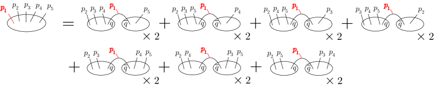
Figure 5: Recursive structure of $W^{(0,5)}(p_{1},\ldots,p_{5})$

By the recursion (3.2), the multilinear meromorphic differentials with the Euler number $\chi=-3$ are obtained. Let us expand these differentials on the character variety (3.34) in terms of the kernel differentials (3.15). After some computation as in appendix B we obtain the meromorphic differential $W^{(0,5)}(p_{1},\ldots,p_{5})$ as follows (see also Fig.5):

$$W^{(0,5)}(p_{1},\ldots,p_{5}) =\sum_{q_{i}\in{\cal C}}\mathop{\mbox{Res}}_{q=q_{i}}\frac{dE_{q,\bar{q}}(p_{1})}{y(q)dq}\Big{\{}\big{(}B(q,p_{2})W^{(0,4)}(\bar{q},p_{3},p_{4},p_{5})+\mbox{perm}(p_{2},p_{3},p_{4},p_{5})\big{)}$$

$$\hskip 72.00014pt+\big{(}W^{(0,3)}(q,p_{2},p_{3})W^{(0,3)}(\bar{q},p_{4},p_{5})+(p_{3}\leftrightarrow p_{4})+(p_{3}\leftrightarrow p_{5})\big{)}\Big{\}}$$

$$=\frac{3}{8}\sum_{i}\Big{\{}M_{i}^{2}\sigma^{\prime}_{i}\big{(}5E_{i}^{2}+10(3A_{i}-a_{i})E_{i}+24A_{i}^{2}+20B_{i}+\frac{10}{3}b_{i}\big{)}\chi_{i\hskip 0.83997pti\hskip 0.83997pti\hskip 0.83997pti\hskip 0.83997pti}^{11111}$$

$$\hskip 8.00002pt+\sum_{j\neq i}M_{i}M_{j}\big{(}H_{ij}(E_{j}+3A_{j}-a_{j})-\frac{\sigma_{i}^{\prime}}{3(q_{i}-q_{j})^{2}}\big{)}\big{[}\chi_{i\hskip 0.83997pti\hskip 0.28001ptj\hskip 0.28001ptj\hskip 0.28001ptj}^{11111}+\mbox{perm}({}_{5}C_{2})\big{]}$$

$$\hskip 8.00002pt+\sum_{j,k\neq i}\frac{M_{j}M_{k}H_{ij}H_{ik}}{3\sigma_{i}^{\prime}}\big{[}\chi_{i\hskip 0.28001ptj\hskip 0.28001ptj\hskip 0.28001ptk\hskip 0.28001ptk}^{11111}+\mbox{perm}(\frac{5!}{2!2!2})\big{]}$$

$$\hskip 8.00002pt+2M_{i}^{2}\sigma^{\prime}_{i}\big{(}3E_{i}+10A_{i}\big{)}\big{[}\chi_{i\hskip 0.83997pti\hskip 0.83997pti\hskip 0.83997pti\hskip 0.83997pti}^{11112}+\mbox{perm}({}_{5}C_{1})\big{]}+\sum_{j\neq i}M_{i}M_{j}H_{ij}\big{[}\chi_{i\hskip 0.83997pti\hskip 0.28001ptj\hskip 0.28001ptj\hskip 0.28001ptj}^{11112}+\mbox{perm}({}_{4}C_{2}\times 5)\big{]}$$

$$\hskip 8.00002pt+6M_{i}^{2}\sigma^{\prime}_{i}\big{[}\chi_{i\hskip 0.83997pti\hskip 0.83997pti\hskip 0.83997pti\hskip 0.83997pti}^{11122}+\mbox{perm}({}_{5}C_{2})\big{]}+5M_{i}^{2}\sigma^{\prime}_{i}\big{[}\chi_{i\hskip 0.83997pti\hskip 0.83997pti\hskip 0.83997pti\hskip 0.83997pti}^{11113}+\mbox{perm}({}_{5}C_{1})\big{]}\Big{\}}.$$ (D.1)

We have defined

$$\chi_{\hskip 0.70004pti_{1}\hskip 1.39998pti_{2}\hskip 0.70004pt\ldots\hskip 1.04996pti_{h}}^{n_{1}n_{2}\ldots n_{h}}:=\chi_{i_{1}}^{(n_{1})}(p_{1})\chi_{i_{2}}^{(n_{2})}(p_{2})\cdots\chi_{i_{h}}^{(n_{h})}(p_{h}),$$ (D.3)

$$a_{i}:=\frac{\sigma_{i}^{\prime\prime}}{3\sigma_{i}^{\prime}}+\frac{M_{i}^{\prime}}{M_{i}},\quad A_{i}:=\frac{\sigma_{i}^{\prime\prime}}{4\sigma_{i}^{\prime}}+\frac{M_{i}^{\prime}}{M_{i}},\quad b_{i}:=\frac{\sigma_{i}^{\prime\prime 2}}{32\sigma_{i}^{\prime 2}}-\frac{\sigma_{i}^{\prime\prime\prime}}{12\sigma_{i}^{\prime}},$$

$$B_{i}:=\frac{M_{i}^{\prime\prime}}{2M_{i}}+\frac{\sigma_{i}^{\prime\prime}M_{i}}{4\sigma_{i}^{\prime}M_{i}}-b_{i},\quad E_{i}:=\frac{1}{\sigma_{i}^{\prime}}\big{(}G-\frac{1}{12}\sigma_{i}^{\prime\prime}\big{)},\quad H_{ij}:=G+\frac{2f(q_{i},q_{j})}{(q_{i}-q_{j})^{2}},$$

where $G=G(k)$, and $f(p,q)$ are defined in (3.26), and (3.28) respectively. In (D.1), “perm” denotes the permutation of $p_{1},\ldots,p_{5}$ so that the result becomes symmetric for these variables, for example,

$$\chi_{i\hskip 0.28001ptj\hskip 0.28001ptj\hskip 0.28001ptk\hskip 0.28001ptk}^{11111}+\mbox{perm}(\frac{5!}{2!2!2}) =\chi_{i\hskip 0.28001ptj\hskip 0.28001ptj\hskip 0.28001ptk\hskip 0.28001ptk}^{11111}+\chi_{j\hskip 0.28001pti\hskip 0.28001ptj\hskip 0.28001ptk\hskip 0.28001ptk}^{11111}+\chi_{j\hskip 0.28001ptj\hskip 0.28001pti\hskip 0.28001ptk\hskip 0.28001ptk}^{11111}+\chi_{k\hskip 0.28001ptj\hskip 0.28001ptj\hskip 0.28001pti\hskip 0.28001ptk}^{11111}+\chi_{k\hskip 0.28001ptj\hskip 0.28001ptj\hskip 0.28001ptk\hskip 0.28001pti}^{11111}+\chi_{i\hskip 0.28001ptk\hskip 0.28001ptj\hskip 0.28001ptj\hskip 0.28001ptk}^{11111}+\chi_{k\hskip 0.28001pti\hskip 0.28001ptj\hskip 0.28001ptj\hskip 0.28001ptk}^{11111}$$

$$+\chi_{k\hskip 0.28001ptj\hskip 0.28001pti\hskip 0.28001ptj\hskip 0.28001ptk}^{11111}+\chi_{k\hskip 0.28001ptk\hskip 0.28001ptj\hskip 0.28001pti\hskip 0.28001ptj}^{11111}+\chi_{k\hskip 0.28001ptk\hskip 0.28001ptj\hskip 0.28001ptj\hskip 0.28001pti}^{11111}+\chi_{i\hskip 0.28001ptj\hskip 0.28001ptk\hskip 0.28001ptj\hskip 0.28001ptk}^{11111}+\chi_{k\hskip 0.28001pti\hskip 0.28001ptj\hskip 0.28001ptk\hskip 0.28001ptj}^{11111}+\chi_{j\hskip 0.28001ptk\hskip 0.28001pti\hskip 0.28001ptj\hskip 0.28001ptk}^{11111}+\chi_{j\hskip 0.28001ptk\hskip 0.28001ptj\hskip 0.28001pti\hskip 0.28001ptk}^{11111}+\chi_{j\hskip 0.28001ptk\hskip 0.28001ptj\hskip 0.28001ptk\hskip 0.28001pti}^{11111}.$$ (D.4)

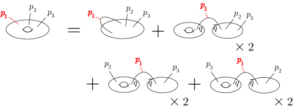
Figure 6: Recursive structure of $W^{(1,3)}(p_{1},p_{2},p_{3})$

In the same way we obtain the meromorphic differential $W^{(1,3)}(p_{1},p_{2},p_{3})$ as follows (see also Fig.6):

$$W^{(1,3)}(p_{1},p_{2},p_{3})=\sum_{q_{i}\in{\cal C}}\mathop{\mbox{Res}}_{q=q_{i}}\frac{dE_{q,\bar{q}}(p_{1})}{2y(q)dq}\Big{\{}W^{(0,4)}(q,\bar{q},p_{2},p_{3})+2W^{(1,1)}(q)W^{(0,3)}(\bar{q},p_{2},p_{3})$$

$$\hskip 168.00032pt+2\big{(}B(q,p_{2})W^{(1,2)}(\bar{q},p_{3})+(p_{2}\leftrightarrow p_{3})\big{)}\Big{\}}$$

$$=\frac{1}{64}\sum_{i}\Big{\{}\big{(}32E_{i}^{3}+(252A_{i}-195a_{i})E_{i}^{2}+(522A_{i}^{2}-846A_{i}a_{i}+318a_{i}^{2}+120B_{i}+92b_{i})E_{i}$$

$$\quad-30A_{i}B_{i}+332A_{i}b_{i}-262a_{i}b_{i}+35(\frac{\sigma_{i}^{\prime\prime}}{2\sigma_{i}^{\prime}}-\frac{2M_{i}^{\prime}}{M_{i}})b_{i}+\frac{3\sigma_{i}^{\prime\prime\prime\prime}}{8\sigma_{i}^{\prime}}+\frac{35\sigma_{i}^{\prime\prime}M_{i}^{\prime\prime}}{4\sigma_{i}^{\prime}M_{i}}+\frac{35M_{i}^{\prime\prime\prime}}{3M_{i}}\big{)}\chi_{i\hskip 0.83997pti\hskip 0.83997pti}^{111}$$

$$+\sum_{j\neq i}\frac{M_{i}}{\sigma_{j}^{\prime}M_{j}}\big{(}(3E_{i}+6A_{i}-\frac{\sigma_{i}^{\prime\prime}}{4\sigma_{i}^{\prime}})(4E_{j}-a_{j})H_{ij}-\frac{\sigma_{i}^{\prime}(E_{i}+2A_{i})+\frac{1}{4}\sigma_{i}^{\prime\prime}+\sigma_{j}^{\prime}(4E_{j}-a_{j})}{(q_{i}-q_{j})^{2}}+\frac{2\sigma_{i}^{\prime}}{(q_{i}-q_{j})^{3}}\big{)}\chi_{i\hskip 0.83997pti\hskip 0.83997pti}^{111}$$

$$+\sum_{j\neq i}\big{(}12(E_{j}+3A_{j}-2a_{j})\frac{H_{ij}^{2}}{\sigma_{i}^{\prime}\sigma_{j}^{\prime}}+(8E_{i}^{2}+(36A_{i}-37a_{i})E_{i}+6A_{i}^{2}-15A_{i}a_{i}+9a_{i}^{2}+\frac{28}{3}b_{i})\frac{M_{j}H_{ij}}{\sigma_{i}^{\prime}M_{i}}$$

$$\quad-\frac{8H_{ij}}{\sigma_{j}^{\prime}(q_{i}-q_{j})^{2}}-\frac{(4E_{i}+2A_{i}-3a_{i})\sigma_{j}^{\prime}M_{j}}{\sigma_{i}^{\prime}M_{i}(q_{i}-q_{j})^{2}}+\frac{\sigma_{j}^{\prime}M_{j}}{\sigma_{i}^{\prime}M_{i}(q_{i}-q_{j})^{3}}\big{)}\big{[}\chi_{i\hskip 0.28001ptj\hskip 0.28001ptj}^{111}+\mbox{perm}({}_{3}C_{1})\big{]}$$

$$+\sum_{j,k\neq i}\frac{M_{j}H_{ij}}{\sigma_{i}^{\prime}\sigma_{k}^{\prime}M_{k}}\big{(}(4E_{k}-a_{k})H_{ik}-\frac{\sigma_{i}^{\prime}}{3(q_{i}-q_{k})^{2}}\big{)}\big{[}\chi_{i\hskip 0.28001ptj\hskip 0.28001ptj}^{111}+\mbox{perm}({}_{3}C_{1})\big{]}+\sum_{j\neq i,k\neq j}\frac{4M_{k}H_{ij}^{2}H_{jk}}{\sigma_{i}^{\prime}\sigma_{j}^{\prime 2}M_{j}}\big{[}\chi_{i\hskip 0.28001ptk\hskip 0.28001ptk}^{111}+\mbox{perm}({}_{3}C_{1})\big{]}$$

$$+\sum_{j\neq i,k\neq i,j}\frac{8H_{ij}H_{jk}H_{ki}}{\sigma_{i}^{\prime}\sigma_{j}^{\prime}\sigma_{k}^{\prime}}\chi_{i\hskip 0.28001ptj\hskip 0.28001ptk}^{111}+2\big{(}24E_{i}^{2}+(121A_{i}-75a_{i})E_{i}-9A_{i}^{2}+25B_{i}+25b_{i}\big{)}\big{[}\chi_{i\hskip 0.83997pti\hskip 0.83997pti}^{112}+\mbox{perm}({}_{3}C_{1})\big{]}$$

$$+\sum_{j\neq i}\frac{3M_{i}}{\sigma_{j}^{\prime}M_{j}}\big{(}(4E_{j}-a_{j})H_{ij}-\frac{\sigma_{i}^{\prime}}{3(q_{i}-q_{j})^{2}}\big{)}\big{[}\chi_{i\hskip 0.83997pti\hskip 0.83997pti}^{112}+\mbox{perm}({}_{3}C_{1})\big{]}+\sum_{j\neq i}\frac{12H_{ij}^{2}}{\sigma_{i}^{\prime}\sigma_{j}^{\prime}}\big{[}\chi_{i\hskip 0.28001ptj\hskip 0.28001ptj}^{112}+\mbox{perm}({}_{3}P_{3})\big{]}$$

$$+\sum_{j\neq i}\frac{M_{j}}{\sigma_{i}^{\prime}M_{i}}\big{(}(12E_{i}+2A_{i}-3a_{i})H_{ij}-\frac{\sigma_{j}^{\prime}}{(q_{i}-q_{j})^{2}}\big{)}\big{[}\chi_{i\hskip 0.28001ptj\hskip 0.28001ptj}^{211}+\mbox{perm}({}_{3}C_{1})\big{]}$$

$$+5\big{(}\frac{13G}{\sigma_{i}^{\prime}}+\frac{2\sigma_{i}^{\prime\prime}}{3\sigma_{i}^{\prime}}+\frac{7M_{i}^{\prime}}{M_{i}}\big{)}\big{[}\chi_{i\hskip 0.83997pti\hskip 0.83997pti}^{113}+\mbox{perm}({}_{3}C_{1})\big{]}+\sum_{j\neq i}\frac{5M_{i}H_{ij}}{\sigma_{j}^{\prime}M_{j}}\big{[}\chi_{i\hskip 0.83997pti\hskip 0.28001ptj}^{113}+\mbox{perm}({}_{3}C_{1})\big{]}$$

$$+24\big{(}\frac{3G}{\sigma_{i}^{\prime}}+\frac{M_{i}^{\prime}}{M_{i}}\big{)}\big{[}\chi_{i\hskip 0.83997pti\hskip 0.83997pti}^{122}+\mbox{perm}({}_{3}C_{1})\big{]}+18\chi_{i\hskip 0.83997pti\hskip 0.83997pti}^{222}+30\big{[}\chi_{i\hskip 0.83997pti\hskip 0.83997pti}^{123}+\mbox{perm}({}_{3}P_{3})\big{]}+35\big{[}\chi_{i\hskip 0.83997pti\hskip 0.83997pti}^{114}+\mbox{perm}({}_{3}C_{1})\big{]}\Big{\}}.$$ (D.5)

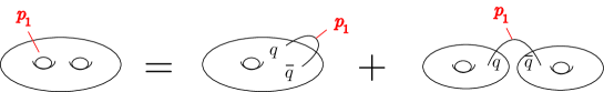
Figure 7: Recursive structure of $W^{(2,1)}(p_{1})$

The meromorphic differential $W^{(2,1)}(p_{1})$ is obtained as follows (see also Fig.7):

$$W^{(2,1)}(p_{1})=\sum_{q_{i}\in{\cal C}}\mathop{\mbox{Res}}_{q=q_{i}}\frac{dE_{q,\bar{q}}(p_{1})}{2y(q)dq}\Big{\{}W^{(1,2)}(q,\bar{q})+W^{(1,1)}(q)W^{(1,1)}(\bar{q})\Big{\}}$$

$$=\frac{1}{64}\sum_{i}\frac{1}{\sigma_{i}^{\prime}M_{i}^{2}}\Big{\{}\big{(}5E_{i}^{4}+(48A_{i}-55a_{i})E_{i}^{3}+(\frac{381}{2}A_{i}^{2}-423A_{i}a_{i}+\frac{3769}{16}a_{i}^{2}-\frac{5}{2}B_{i}+\frac{191}{6}b_{i})E_{i}^{2}$$

$$\quad+(135A_{i}^{3}-\frac{1767}{4}A_{i}^{2}a_{i}+(\frac{3975}{8}a_{i}^{2}-15B_{i}+211b_{i})A_{i}-\frac{1521}{8}a_{i}^{3}+15a_{i}B_{i}-\frac{1399}{6}a_{i}b_{i}-\frac{31\sigma_{i}^{\prime\prime\prime\prime}}{48\sigma_{i}^{\prime}})E_{i}$$

$$\quad+\frac{417}{2}A_{i}^{2}b_{i}-466A_{i}a_{i}b_{i}-\frac{109\sigma_{i}^{\prime\prime\prime\prime}}{96\sigma_{i}^{\prime}}A_{i}+\frac{267\sigma_{i}^{\prime\prime\prime\prime}}{192\sigma_{i}^{\prime}}a_{i}+\frac{2109}{8}a_{i}^{2}b_{i}-5B_{i}b_{i}+\frac{190}{9}b_{i}^{2}\big{)}\chi_{i}^{1}$$

$$+\sum_{j\neq i}\big{(}\frac{M_{i}}{2\sigma_{i}^{\prime}\sigma_{j}^{\prime 2}M_{j}}(12E_{i}+24A_{i}-25a_{i})H_{ij}^{3}+\frac{M_{i}^{2}}{2\sigma_{j}^{\prime 2}M_{j}^{2}}(\frac{1}{8}(4E_{j}-a_{j})^{2}+(8E_{j}+36A_{j}-49a_{j})E_{j}+15A_{j}^{2}$$

$$\quad-30A_{j}a_{j}+21a_{j}^{2}-5B_{j}+\frac{31}{3}b_{j})H_{ij}^{2}-\frac{25M_{i}H_{ij}^{2}}{6(q_{i}-q_{j})^{2}\sigma_{i}^{\prime}\sigma_{j}^{\prime}M_{j}}-\frac{\sigma_{i}^{\prime}M_{i}^{2}}{2(q_{i}-q_{j})^{2}\sigma_{j}^{\prime 2}M_{j}^{2}}(\frac{25}{3}E_{j}+4A_{j}-\frac{97}{12}a_{j}$$

$$\quad+\frac{2}{q_{i}-q_{j}})H_{ij}+\frac{M_{i}}{2\sigma_{j}^{\prime}M_{j}}(4E_{j}-a_{j})(2E_{i}^{2}+(9A_{i}-\frac{37}{4}a_{i})E_{i}+\frac{3}{2}A_{i}^{2}-\frac{15}{4}A_{i}a_{i}+\frac{9}{4}a_{i}^{2}+\frac{7}{3}b_{i})H_{ij}$$

$$\quad+\frac{25\sigma_{i}^{\prime 2}M_{i}^{2}}{144(q_{i}-q_{j})^{4}\sigma_{j}^{\prime 2}M_{j}^{2}}-\frac{\sigma_{i}^{\prime}M_{i}}{6(q_{i}-q_{j})^{2}\sigma_{j}^{\prime}M_{j}}(E_{i}^{2}+6(A_{i}-a_{i})E_{i}+2b_{i})+\frac{\sigma_{i}^{\prime}M_{i}}{8(q_{i}-q_{j})^{2}\sigma_{j}^{\prime}M_{j}}(-\frac{4}{3}E_{i}^{2}$$

$$\quad+(12A_{i}-\frac{35}{3}a_{i})E_{i}-3A_{i}^{2}+3A_{i}a_{i}+\frac{14}{9}b_{i}-(4E_{i}+2A_{i}-3a_{i})(4E_{j}-a_{j})\frac{\sigma_{j}^{\prime}}{\sigma_{i}^{\prime}}+\frac{1}{q_{i}-q_{j}}(8E_{i}-12A_{i}$$

$$\quad+10a_{i}+(4E_{j}-a_{j})\frac{\sigma_{j}^{\prime}}{\sigma_{i}^{\prime}})-\frac{5}{(q_{i}-q_{j})^{2}})\big{)}\chi_{i}^{1}$$

$$+\sum_{j\neq i,k\neq i,j}\frac{M_{i}^{2}}{\sigma_{j}^{\prime 2}\sigma_{k}^{\prime 2}M_{j}M_{k}}\big{(}(4H_{ik}H_{jk}^{2}+\sigma_{k}^{\prime}(4E_{k}-a_{k})H_{ij}H_{jk}-\frac{\sigma_{j}^{\prime}\sigma_{k}^{\prime}H_{ij}}{3(q_{j}-q_{k})^{2}})\frac{H_{ij}}{2}$$

$$\quad+\sigma_{j}^{\prime}\sigma_{k}^{\prime}((E_{j}-\frac{1}{4}a_{j})H_{ij}-\frac{\sigma_{i}^{\prime}}{12(q_{i}-q_{j})^{2}})((E_{k}-\frac{1}{4}a_{k})H_{ik}-\frac{\sigma_{i}^{\prime}}{12(q_{i}-q_{k})^{2}})\big{)}\chi_{i}^{1}$$

$$+\big{(}10E_{i}^{3}+(61A_{i}-75a_{i})E_{i}^{2}+(45A_{i}^{2}-\frac{409}{4}A_{i}a_{i}+\frac{507}{8}a_{i}^{2}-5B_{i}+31b_{i})E_{i}+\frac{121}{3}A_{i}b_{i}-\frac{97}{2}a_{i}b_{i}-\frac{73\sigma_{i}^{\prime\prime\prime\prime}}{384\sigma_{i}^{\prime}}\big{)}\chi_{i}^{2}$$

$$+\sum_{j\neq i}\frac{M_{i}}{\sigma_{j}^{\prime}M_{j}}\big{(}\frac{4H_{ij}^{3}}{\sigma_{i}^{\prime}\sigma_{j}^{\prime}}+(\frac{3}{2}E_{i}+\frac{1}{4}A_{i}-\frac{3}{8}a_{i})(4E_{j}-a_{j})H_{ij}+\frac{\sigma_{i}^{\prime}}{4(q_{i}-q_{j})^{3}}$$

$$\quad-\frac{\sigma_{i}^{\prime}}{(q_{i}-q_{j})^{2}}(\frac{1}{2}E_{i}-\frac{5}{12}A_{i}+\frac{3}{8}a_{i}+\frac{(4E_{j}-a_{j})\sigma_{j}^{\prime}}{8\sigma_{i}^{\prime}})\big{)}\chi_{i}^{2}$$

$$+\big{(}\frac{35}{2}E_{i}^{2}+(\frac{35}{2}A_{i}-\frac{245}{8}a_{i})E_{i}+\frac{49}{16}A_{i}^{2}-\frac{5}{2}B_{i}+\frac{245}{24}b_{i}\big{)}\chi_{i}^{3}+\sum_{j\neq i}\frac{M_{i}}{\sigma_{j}^{\prime}M_{j}}\big{(}\frac{5}{8}(4E_{j}-a_{j})H_{ij}-\frac{5\sigma_{i}^{\prime}}{24(q_{i}-q_{j})^{2}}\big{)}\chi_{i}^{3}$$

$$+\big{(}\frac{35}{2}E_{i}-\frac{49}{8}A_{i}\big{)}\chi_{i}^{4}+\frac{105}{16}\chi_{i}^{5}\Big{\}}.$$ (D.6)

D.1 Figure eight knot complement

The free energies (3.47) with $\chi=-3$ on the curve (3.59), (3.60) for the figure eight knot complement are summarized as follows:

$${\cal F}^{(0,5)}(p)=\frac{1}{{\widetilde{\sigma}}(w)^{9/2}}\Big{(}-\frac{4}{3}w^{8}+\frac{10}{3}w^{7}-3w^{6}-\frac{119}{6}w^{5}+\frac{2273}{60}w^{4}-\frac{997}{120}w^{3}-\frac{9271}{240}w^{2}+\frac{6357}{160}w-\frac{1411}{120}\Big{)},$$ (D.7)

$${\cal F}^{(1,3)}(p)=-\frac{(4w-3)^{3}G_{3}}{162000{\widetilde{\sigma}}(w)^{3/2}}-\frac{(4w-3)G_{2}}{300{\widetilde{\sigma}}(w)^{5/2}}\Big{(}\frac{16}{27}w^{4}-\frac{58}{27}w^{3}+\frac{13}{9}w^{2}+\frac{7}{2}w-\frac{9}{4}\Big{)}$$

$$-\frac{G_{1}}{{\widetilde{\sigma}}(w)^{7/2}}\Big{(}\frac{2368}{30375}w^{7}-\frac{17714}{30375}w^{6}+\frac{29443}{30375}w^{5}+\frac{106}{81}w^{4}-\frac{1267}{450}w^{3}-\frac{3239}{9000}w^{2}+\frac{21823}{6000}w-\frac{3637}{2000}\Big{)}$$

$$-\frac{1}{{\widetilde{\sigma}}(w)^{9/2}}\Big{(}\frac{15616}{54675}w^{9}-\frac{60448}{18225}w^{8}+\frac{139624}{18225}w^{7}+\frac{103012}{10935}w^{6}-\frac{19846}{2025}w^{5}-\frac{23747}{675}w^{4}+\frac{85901}{1350}w^{3}$$

$$\hskip 40.00008pt+\frac{4151}{300}w^{2}-\frac{3277}{40}w+\frac{140863}{3600}\Big{)},$$ (D.8)

$${\cal F}^{(2,1)}(p)=-\frac{4(4w-3){\widetilde{G}}_{3}}{50625{\widetilde{\sigma}}(w)^{1/2}}+\frac{{\widetilde{G}}_{2}}{900{\widetilde{\sigma}}(w)^{5/2}}\Big{(}\frac{2944}{135}w^{5}-\frac{8807}{135}w^{4}+\frac{1003}{54}w^{3}+\frac{13813}{180}w^{2}-\frac{559}{24}w-\frac{85}{2}\Big{)}$$

$$+\frac{{\widetilde{G}}_{1}}{1125{\widetilde{\sigma}}(w)^{7/2}}\Big{(}\frac{88448}{405}w^{7}-\frac{24656}{27}w^{6}+\frac{106688}{135}w^{5}+\frac{349636}{405}w^{4}-\frac{104866}{135}w^{3}-\frac{6142}{5}w^{2}-\frac{187}{30}w+\frac{11311}{10}\Big{)}$$

$$+\frac{1}{5625{\widetilde{\sigma}}(w)^{9/2}}\Big{(}\frac{827392}{243}w^{9}-\frac{4380472}{243}w^{8}+\frac{1967444}{81}w^{7}+\frac{3066698}{243}w^{6}-\frac{11109413}{243}w^{5}+\frac{13223}{54}w^{4}$$

$$\hskip 40.00008pt-\frac{2184931}{108}w^{3}+\frac{3318629}{72}w^{2}+\frac{786203}{16}w-\frac{451859}{8}\Big{)},$$ (D.9)

where by distinguishing $G$ in ${\cal F}^{(1,3)}(p)$ from $G$ in ${\cal F}^{(2,1)}(p)$, we put $G_{1}=G,~{}G_{2}=G^{2},~{}G_{3}=G^{3}$ in (D.8), and ${\widetilde{G}}_{1}=G,~{}{\widetilde{G}}_{2}=G^{2},~{}{\widetilde{G}}_{3}=G^{3}$ in (D.9). If we regularize these parameters as

$$G_{1}=\frac{7}{3},\quad G_{2}=-\frac{95}{9},\quad G_{3}=\Big{(}\frac{7}{3}\Big{)}^{3},\quad{\widetilde{G}}_{1}=\frac{7}{3},\quad{\widetilde{G}}_{2}=-\frac{47}{9},\quad{\widetilde{G}}_{3}=-\frac{131}{27},$$ (D.10)

then the free energy

$${\cal F}_{4}(p) = 4\big{(}{\cal F}^{(0,5)}(p)+{\cal F}^{(1,3)}(p)+{\cal F}^{(2,1)}(p)\big{)}$$ (D.11)

$$= \frac{1}{{15\widetilde{\sigma}}(w)^{9/2}}\Big{(}\frac{128}{3}w^{8}-\frac{256}{3}w^{7}-\frac{4352}{3}w^{6}+\frac{1024}{3}w^{5}+\frac{14896}{3}w^{4}$$

$$\hskip 50.00008pt-\frac{23464}{3}w^{3}+212w^{2}+8194w-\frac{27469}{6}\Big{)}$$

coincides with the perturbative invariant (2.38), where $w=(m^{2}+m^{-2})/2$.

D.2 Once punctured torus bundle over $\mathbb{S}^{1}$ with holonomy $L^{2}R$

The free energies (3.47) with $\chi=-3$ on the curve (3.71), (3.72) for the once punctured torus bundle over $\mathbb{S}^{1}$ with holonomy $L^{2}R$ are summarized as follows:

$${\cal F}^{(0,5)}(p)=\frac{1}{{\widetilde{\sigma}}(w)^{9/2}}\Big{(}-\frac{4}{3}w^{8}-\frac{58}{3}w^{6}-\frac{23}{2}w^{5}+\frac{319}{20}w^{4}-\frac{2069}{60}w^{3}-\frac{47}{12}w^{2}+\frac{13651}{480}w-\frac{5341}{480}\Big{)},$$ (D.12)

$${\cal F}^{(1,3)}(p)=-\frac{(6w-7)^{3}G_{3}}{1053696{\widetilde{\sigma}}(w)^{3/2}}-\frac{(6w-7)G_{2}}{784{\widetilde{\sigma}}(w)^{5/2}}\Big{(}\frac{3}{7}w^{4}-\frac{17}{7}w^{3}+\frac{17}{6}w^{2}+\frac{71}{12}w-\frac{133}{48}\Big{)}$$

$$-\frac{G_{1}}{{8\widetilde{\sigma}}(w)^{7/2}}\Big{(}\frac{45}{343}w^{7}-\frac{1727}{686}w^{6}+\frac{27595}{4116}w^{5}+\frac{42659}{3528}w^{4}-\frac{181607}{7056}w^{3}+\frac{33499}{2016}w^{2}+\frac{134411}{4032}w-\frac{20671}{1152}\Big{)}$$

$$+\frac{1}{{\widetilde{\sigma}}(w)^{9/2}}\Big{(}\frac{89}{1029}w^{9}-\frac{1515}{686}w^{8}+\frac{8870}{1029}w^{7}+\frac{956534}{27783}w^{6}-\frac{77521}{10584}w^{5}+\frac{38095}{784}w^{4}+\frac{37477}{324}w^{3}$$

$$\hskip 40.00008pt-\frac{35419}{336}w^{2}-\frac{558557}{6912}w+\frac{2672231}{41472}\Big{)},$$ (D.13)

$${\cal F}^{(2,1)}(p)=\frac{81(6w-7){\widetilde{G}}_{3}}{2458624{\widetilde{\sigma}}(w)^{1/2}}+\frac{{\widetilde{G}}_{2}}{224{\widetilde{\sigma}}(w)^{5/2}}\Big{(}\frac{981}{343}w^{5}-\frac{6101}{686}w^{4}-\frac{3911}{686}w^{3}+\frac{6605}{196}w^{2}-\frac{471}{112}w-\frac{1063}{32}\Big{)}$$

$$-\frac{{\widetilde{G}}_{1}}{56{\widetilde{\sigma}}(w)^{7/2}}\Big{(}\frac{1629}{343}w^{7}-\frac{16263}{686}w^{6}+\frac{20913}{1372}w^{5}+\frac{194077}{2744}w^{4}-\frac{53455}{784}w^{3}-\frac{42725}{224}w^{2}+\frac{4253}{64}w+\frac{21273}{128}\Big{)}$$

$$+\frac{1}{98{\widetilde{\sigma}}(w)^{9/2}}\Big{(}\frac{1115}{49}w^{9}-\frac{123383}{2205}w^{8}+\frac{123383}{2205}w^{7}+\frac{2396633}{4410}w^{6}-\frac{24202151}{17640}w^{5}-\frac{2692853}{720}w^{4}$$

$$\hskip 40.00008pt+\frac{751187}{720}w^{3}+\frac{8009701}{1440}w^{2}-\frac{6519401}{11520}w-\frac{14175847}{4608}\Big{)},$$ (D.14)

where as in the case of the figure eight knot complement, we distinguished $G$ in ${\cal F}^{(1,3)}(p)$ from $G$ in ${\cal F}^{(2,1)}(p)$. In this example, as in (2.62) the partition function for the state integral model contains imaginary terms. Therefore we have to add the imaginary term to our result for the comparison with (2.64), but we do not find natural regularizations for the above $G$’s, and natural choice of the imaginary term. We leave the problem to future work.

References

- [1] E. Witten, “Quantum Field Theory and the Jones Polynomial,” Commun. Math. Phys. 121 (1989) 351.
- [2] E. Witten, “(2+1)-Dimensional Gravity as an Exactly Soluble System,” Nucl. Phys. B311 (1998) 46.
- [3] R. M. Kashaev, “The Hyperbolic Volume of Knots from the Quantum Dilogarithm,” Lett. Math. Phys. 39 (1997) no. 3, 269-275.
- [4] H. Murakami and J. Murakami, “The Colored Jones Polynomials and the Simplicial Volume of a Knot,” Acta Math. 186 (2001) no. 1, 85-104, arXiv:math/9905075 [math.GT].
- [5] S. Gukov, “Three-dimensional quantum gravity, Chern-Simons theory, and the A-polynomial,” Commun. Math. Phys. 255 (2005) 577-627, arXiv:hep-th/0306165.
- [6] S. Gukov and H. Murakami, “ Chern-Simons Theory and the Asymptotic Behavior of the Colored Jones Polynomial,” arXiv:math/0608324v2 [math.GT].
- [7] J. Porti, “Torsion de Reidemeister pour les variétés hyperboliques,” vol. 128, Mem. Amer. Math. Soc. 612 AMS, 1997.
- [8] R. Dijkgraaf and H. Fuji, “The volume conjecture and topological strings,” Fortsch. Phys. 57 (2009) 825-856, arXiv:0903.2084 [hep-th].
- [9] D. Cooper, M. Culler, H. Gillet, D. D. Long and P. B. Shalen, “Plane Curves Associated to Character Varieties of -manifolds,” Invent. Math. 118 (1994) 47–84.
- [10] M. Hildebrand and J. Weeks, “A computer generated census of cusped hyperbolic 3-manifolds,” Computers and Mathematics (E. Kaltofen and S. Watt, eds.), Springer-Verlag, (1989) 53-59.
- [11] M. D. Baker and A. W. Reid, “Arithmetic knots in closed 3-manifolds,” J. Knot Theory Ramifications, 11 (2002) 903-920.
- [12] M. Bruno and P. Carlo, “Dehn filling of the “magic” 3-manifold,” Comm. Anal. Geom. 14 (2006) 969–1026, arXiv:math/0204228.
- [13] D. Futer, E. Kalfagianni and J. S. Purcell, “Symmetric links and Conway sums: volume and Jones polynomial,” Math. Res. Lett. 16 (2009) 233-253, arXiv:0804.1542 [math.GT].
- [14] M. Mariño, “Open string amplitudes and large order behavior in topological string theory,” JHEP 0803 (2008) 060, arXiv:hep-th/0612127.
- [15] V. Bouchard, A. Klemm, M. Mariño and S. Pasquetti, “Remodeling the B-model,” Commun. Math. Phys. 287 (2009) 117-178, arXiv:0709.1453 [hep-th].
- [16] B. Eynard and N. Orantin, “Invariants of Algebraic Curves and Topological Expansion,” Commun. Number Theory Phys. 1 (2007) 347-452, arXiv:math-ph/0702045.
- [17] R. Dijkgraaf and C. Vafa, “Two Dimensional Kodaira-Spencer Theory and Three Dimensional Chern-Simons Gravity,” arXiv:0711.1932 [hep-th].
- [18] V. Bouchard, A. Klemm, M. Marino and S. Pasquetti, “Topological open strings on orbifolds,” Commun. Math. Phys. 296, 589 (2010) [arXiv:0807.0597 [hep-th]].
- [19] A. Brini and A. Tanzini, “Exact results for topological strings on resolved singularities,” Commun. Math. Phys. 289 (2009) 205-252, arXiv:0804.2598 [hep-th].
- [20] M. Manabe, “Topological open string amplitudes on local toric del Pezzo surfaces via remodeling the B-model,” Nucl. Phys. B819 (2009) 35-75, arXiv:0903.2092 [hep-th].
- [21] T. Dimofte, S. Gukov, J. Lenells and D. Zagier, “Exact Results for Perturbative Chern-Simons Theory with Complex Gauge Group,” Commun. Num. Theor .Phys. 3 (2009) 363-443, arXiv:0903.2472 [hep-th].
- [22] T. Dimofte and S. Gukov, “Quantum Field Theory and the Volume Conjecture,” arXiv:1003.4808 [math.GT].
- [23] K. Hikami, “Hyperbolic Structure Arising from a Knot Invariant,” Int. J. Mod. Phys. A16 (2001) 3309–3333, arXiv:math-ph/0105039.
- [24] K. Hikami, “Hyperbolic Structure Arising from a Knot Invariant II. Completeness,” Int. J. Mod. Phys. B16 (2002) 1963–1970.
- [25] K. Hikami, “Generalized Volume Conjecture and the A-Polynomials – the Neumann-Zagier Potential Function as a Classical Limit of Quantum Invariant,” J. Geom. Phys. 57 (2007) 1895–1940, arXiv:math/0604094.
- [26] G. Ponzano and T. Regge, “Semiclassical limit of Racah coefficients,” in Spectroscopic and group theoretical methods in physics, Bloch ed. (North-Holland 1968).
- [27] V. G. Turaev and O.Y. Viro, “State sum invariants of -manifolds and quantum -symbols,” Topology 31 (1992), 865–902.
- [28] C. Kozcaz, S. Pasquetti and N. Wyllard, “A & B model approaches to surface operators and Toda theories,” JHEP 1008 (2010) 042. arXiv:1004.2025 [hep-th].
- [29] T. Dimofte, S. Gukov and L. Hollands, “Vortex Counting and Lagrangian 3-manifolds,” arXiv:1006.0977 [hep-th].
- [30] H. Awata, H. Fuji, H. Kanno, M. Manabe and Y. Yamada, “Localization with a Surface Operator, Irregular Conformal Blocks and Open Topological String,” arXiv:1008.0574 [hep-th].
- [31] S. Garoufalidis, “Difference and differential equations for the colored Jones function,” J. Knot Theory Ramifications 17 (2008) 495-510, arXiv:math/0306229 [math.GT].
- [32] S. Garoufalidis, “On the characteristic and deformation varieties of a knot,” Geom. Topol. Monogr. 7 (2004) 291-309, arXiv:math/0306230 [math.GT].
- [33] S. Garoufalidis and T. T. Q. Le, “The Colored Jones Function is q-Holonomic,” Geom. Topol. 9 (2005) 1253-1293, arXiv:math/0309214 [math.GT].
- [34] S. Garoufalidis and J. S. Geronimo, “Asymptotics of -difference equations,” Primes and knots, 83–114, Contemp. Math. 416 Amer. Math. Soc., Providence, RI, 2006.
- [35] K. Hikami, “Difference equation of the colored Jones polynomial for torus knot ,” Int. J. Math. 15 (2004) 959–965, arXiv:math/0403224 [math.GT].
- [36] W. P. Thurston, “The Geometry and Topology of Three-Manifolds,” Electronic version 1.1 - March 2002, http://www.msri.org/publications/books/gt3m/.
- [37] L. Faddeev, “Modular double of a quantum group,” Conférence Moshé Flato 1999, Vol. I (Dijon), 149–156, Math. Phys. Stud. 21 Kluwer Acad. Publ. Dordrecht (2000).
- [38] D. W. Boyd, “Mahler’s Measure and Invariants of Hyperbolic Manifolds,” Number theory for the millennium, I (Urbana, IL, 2000) 127-143, A K Peters, Natick, MA, 2002.
- [39] W. D. Neumann and D. Zagier, “Volumes of Hyperbolic Three-manifolds,” Topology 24 (1985) no. 3, 307-332.
- [40] T. Jorgensen, “On pairs of punctured tori,” In: Komori, Y., Markovic, V., Series, C. (eds.), Kleinian Groups and Hyperbolic 3-Manifolds, London Math. Soc. Lecture Notes, vol. 299, CUP, Cambridge (2003).
- [41] H. Akiyoshi, M. Sakuma, M. Wada and Y. Yamashita, “Punctured torus groups and 2-bridge knot groups (I)” Lecture Notes in Mathematics, 1909. Springer, Berlin (2007).
- [42] W. Floyd and A. Hatcher, “Incompressible surfaces in punctured-torus bundles,” Topology and its Applications, 13 (1982), 263-282.
- [43] J-P. Otal, “Le théorème d’hyperbolisation pour les variétés fibrées de dimension trois,” Astérisque No. 235 (1996).
- [44] F. Guéritaud and D. Futer, “On canonical triangulations of once-punctured torus bundles and two-bridge link complements,” Geom. Topol. 10 (2006) 1239-1284, arXiv:math/0406242 [math.GT].
- [45] A. W. Reid, “Arithmeticity of knot complements,” J. London Math. Soc. 43 (1991) 171-184.
- [46] D. W. Boyd, F. Rodriguez-Villegas and N. M. Dunfield, “Mahler’s Measure and the Dilogarithm (II),” arXiv:math/0308041 [math.NT].
- [47] J. Ambjørn, L. Chekhov, C. F. Kristjansen and Yu. Makeenko, “Matrix model calculations beyond the spherical limit,” Nucl. Phys. B 404 (1993) 127-172; Erratum-ibid. B 449 (1995) 681, arXiv:hep-th/9302014.
- [48] G. Akemann, “Higher genus correlators for the hermitian matrix model with multiple cuts,” Nucl.Phys. B482 (1996) 403-430, arXiv:hep-th/9606004.
- [49] B. Eynard, “Topological expansion for the 1-hermitian matrix model correlation functions,” JHEP 0411 (2004) 031, arXiv:hep-th/0407261.
- [50] T. Yoshida, “The -invariant of Hyperbolic 3-manifolds,” Invent. Math. 81 (1985) no. 3, 473-514.
- [51] H. Morton, The coloured Jones function and Alexander polynomial for torus knots, Math. Proc. Cambridge Philos. Soc. 117 (1995) 129-135.
- [52] P. M. Melvin and H. R. Morton, “The coloured Jones function,” Comm. Math. Phys. 169 (1995) 501-520.
- [53] L. Rozansky, “The universal R-matrix, Burau representation, and the Melvin-Morton expansion of the colored Jones polynomial,” Adv. Math. 134 (1998) 1-31.
- [54] S. Garoufalidis and T. T. Q. Le, “An analytic version of the Melvin-Morton-Rozansky Conjecture,” J. Knot Theory Ramifications 11 (2002) 283-293. arXiv:math/0503641v2 [math.GT].
- [55] L. Rozansky, “Higher Order Terms in the Melvin-Morton Expansion of the Colored Jones Polynomial,” Comm. Math. Phys. 183 (1997) 291-306. arXiv:q-alg/9601009.
- [56] R. M. Kashaev and O. Tirkkonen, “A proof of the volume conjecture on torus knots,” Zap. Nauchn. Sem. S.-Peterburg. Otdel. Mat. Inst. Steklov. (POMI) 269 (2000), no. Vopr. Kvant. Teor. Polya i Stat. Fiz. 16, 262-268, 370. MR 1 805-865, arXiv:math/9912210 [math.GT].
- [57] J. Dubois and R. Kashaev, “On the asymptotic expansion of the colored Jones polynomial for torus knots,”arXiv:math/0510607 [math.GT].
- [58] K. Hikami and H. Murakami, “Representations and the colored Jones polynomial of a torus knot,” arXiv:1001.2680 [math.GT].
- [59] P. Kirk and E. Klassen, “ Chern-Simons invariants of 3-manifolds decomposed along tori and the circle bundle over the representation space of ,” Comm. Math. Phys. 153 (1993) 521-557.
-
[60]
P. Paule, A. Riese, Mathematica software:
http://www.risc.uni-linz.ac.at/research/combinat/risc/software/qZeil/. - [61] E. Witten, “Analytic Continuation Of Chern-Simons Theory,” arXiv:1001.2933 [hep-th].
- [62] V. Bouchard and M. Mariño, “Hurwitz numbers, matrix models and enumerative geometry,” Proc. Symposia Pure Math. 78 (2008) 263-283, arXiv:0709.1458 [math.AG].
- [63] B. Eynard, M. Mulase and B. Safnuk, “The Laplace transform of the cut-and-join equation and the Bouchard-Marino conjecture on Hurwitz numbers,” arXiv:0907.5224 [math.AG].
- [64] L. F. Alday, D. Gaiotto and Y. Tachikawa, “Liouville Correlation Functions from Four-dimensional Gauge Theories,” Lett. Math. Phys. 91, 167 (2010) [arXiv:0906.3219 [hep-th]].
- [65] R. Dijkgraaf, H. Fuji and M. Manabe, work in progress.
- [66] T. Dimofte, private communication.
- [67] R. Dijkgraaf, L. Hollands, P. Sulkowski and C. Vafa, “Supersymmetric Gauge Theories, Intersecting Branes and Free Fermions,” JHEP 0802 106, arXiv:0709.4446 [hep-th].
- [68] R. Dijkgraaf, L. Hollands and P. Sulkowski, “Quantum Curves and D-Modules,” JHEP 0911 (2009) 047, arXiv:0810.4157 [hep-th].