Transition from single-file to two-dimensional diffusion of interacting particles in a quasi-one-dimensional channel

Abstract

Diffusive properties of a monodisperse system of interacting particles confined to a quasi-one-dimensional (Q1D) channel are studied using molecular dynamics (MD) simulations. We calculate numerically the mean-squared displacement (MSD) and investigate the influence of the width of the channel (or the strength of the confinement potential) on diffusion in finite-size channels of different shapes (i.e., straight and circular). The transition from single-file diffusion (SFD) to the two-dimensional diffusion regime is investigated. This transition (regarding the calculation of the scaling exponent ($\alpha$) of the MSD $\langle\Delta x^{2}(t)\rangle$ $\propto t^{\alpha}$) as a function of the width of the channel, is shown to change depending on the channel’s confinement profile. In particular the transition can be either smooth (i.e., for a parabolic confinement potential) or rather sharp/stepwise (i.e., for a hard-wall potential), as distinct from infinite channels where this transition is abrupt. This result can be explained by qualitatively different distributions of the particle density for the different confinement potentials.

I Introduction

There is a considerable theoretical and practical interest in the dynamics of systems of interacting particles in confined geometries bocquet . Single-file diffusion (SFD) refers to a one-dimensional (1D) process where the motion of particles in a narrow channel (e.g., quasi-1D systems) is limited such that particles are not able to cross each other. As a consequence, the system diffuses as a whole resulting in anomalous diffusion. The mechanism of SFD was first proposed by Hodgkin and Keynes hodgkin in order to study the passage of molecules through narrow pores. Since the order of the particles is conserved over time, this results in unusual dynamics of the system kargerPRA ; martin , different from what is predicted from diffusion governed by Fick’s law. The main characteristic of the SFD phenomena is that, in the long-time limit, the MSD (mean-square displacement, defined as $\langle\Delta x^{2}(t)\rangle=\langle\sum_{i=1}^{N}(1/N)[x_{i}(t+\Delta t)-x_{i}(t)]^{2}\rangle_{\Delta t}$) scales with time as

$$\langle\Delta x^{2}(t)\rangle\propto t^{0.5}.$$ (1)

This relation was first obtained analytically in the pioneering work of Harris TEHarris . Recent advances in nanotechnology have stimulated a growing interest in SFD, in particular, in the study of transport in nanopores soaresPRB ; soaresPRL . Ion channels of biological membranes and carbon nanotubes GHummer are examples of such nanopores. The macroscopic flux of particles through such nanopores is of great importance for many practical applications, e.g., particle transport across membranes is a crucial intermediate step in almost all biological and chemical engineering processes. SFD was observed in experiments on diffusion of molecules in zeolite molecular sieves meier . Zeolites with unconnected parallel channels may serve as a good realization of the theoretically investigated one-dimensional systems. SFD is also related to growth phenomena grphen .

The theoretical background of SFD was developed in early studies on transport phenomena in 1D channels lebowitz ; levitt ; richards . It is also interesting to learn how the size of the system will influence the diffusive properties of the system. SFD in finite size systems has been the focus of increasing attention since there are few exact theoretical results to date PRE80-051103 ; PRE80-031118 ; PRL102-050602 , which showed the existence of different regimes of diffusion.

Colloidal systems, complex plasmas and vortex matter in type-II superconductors are examples of systems where SFD may occur. The use of colloidal particles is technically interesting since it allows real time and spatial direct observation of their position, which is a great advantage as compared to atoms or molecules, as shown recently in, e.g., the experimental study of defect induced melting alsayed309 . One typically uses micro-meter size colloidal particles in narrow channels, as shown in weiScience ; PRLsfd . The paramagnetic colloidal spheres of 3.6 $\mu m$ were confined in circular trenches fabricated by photolithography and their trajectories were followed over long periods of time. Several other studies have focused on the diffusive properties of complex plasmas. A complex plasma consists of micrometer-sized (“dust”) particles immersed in a gaseous plasma background. Dust particles typically acquire a negative charge of several thousand elementary charges, and thus they interact with each other through their strong electrostatic repulsion gioPRE .

Systems of particles moving in space of reduced dimensionality or submitted to an external confinement potential exhibit different behavior from their free-of-border counterparts wandPRB . The combined effect of interaction between the particles and the confinement potential plays a crucial role in their physical and chemical properties kwinPRE . In Ref. kwinEPL80 , it was found that SFD depends on the inter-particle interaction and can even be suppressed if the interaction is sufficiently strong, resulting in a slower subdiffusive behavior, where $\langle\Delta x^{2}(t)\rangle$ $\propto t^{\alpha}$, with $\alpha<0.5$.

In this paper, we will investigate the effects of confinement potential on the diffusive properties of a Q1D system of interacting particles. In the limiting case of very narrow (wide) channels, particle diffusion can be referred to SFD (2D regime) characterized by a subdiffusive (normal diffusive) long-time regime where the mean-squared displacement (MSD) $\langle\Delta x^{2}(t)\rangle$ $\propto t^{0.5}$ ($\propto t^{1.0}$). Recall that the MSD of a tagged hard-sphere particle in a one dimensional infinite system is characterized by two limiting diffusion behaviors: for time scales shorter than a certain crossover time $\tau_{c}=1/D\rho^{2}$, where $D$ is the diffusion coefficient and $\rho$ is the particle concentration, $\langle\Delta x^{2}(t)\rangle$ $\propto t^{1.0}$ which is referred to as the normal diffusion regime underdamped . For times larger than $\tau_{c}$, the system exhibits a subdiffusive behavior, with the MSD $\langle\Delta x^{2}(t)\rangle$ $\propto t^{0.5}$, which characterizes the single-file diffusion regime. Between these two regimes, there is a transient regime exhibiting a non-trivial functional form.

However, in case of a finite system of diffusing particles (e.g., a circular chain or a straight chain in the presence of periodic boundary conditions), the SFD regime (i.e., with $\langle\Delta x^{2}(t)\rangle$ $\propto t^{0.5}$) does not hold for $t\rightarrow\infty$, unlike in an infinite system. Instead, for sufficiently long times, the SFD regime turns to the regime of collective diffusion, i.e., when the whole system diffuses as a single “particle” with a renormalized mass. This diffusive behavior has been revealed in experiments weiScience ; MSJ and theoretical studies Tepper ; kwinEPL80 ; submitEPL ; SJNew ; PMCentres . This collective diffusion regime is similar to the initial short-time diffusion regime and it is characterized by either $\langle\Delta x^{2}(t)\rangle$ $\propto t^{1.0}$, for overdamped particles (see, e.g., Tepper ; weiScience ; kwinEPL80 ) or by $\langle\Delta x^{2}(t)\rangle$ $\propto t^{2.0}$ (followed by the MSD $\propto t^{1.0}$), for underdamped systems submitEPL ; SJNew . Correspondingly, the time interval where the SFD regime is observed becomes finite in finite size systems. It depends on the lenght of the chain of diffusing particles: the longer the chain the longer the SFD time interval. Therefore, in order to observe a clear power-law behavior (i.e., $\langle\Delta x^{2}(t)\rangle$ $\propto t^{\alpha}$) one should consider sufficiently large systems.

Here we focus on this intermediate diffusion regime and we show that it can be characterized by $\langle\Delta x^{2}(t)\rangle$ $\propto t^{\alpha}$, where $0.5<\alpha<1.0$, depending on the width (or the strenght of the confinement potential) of the channel. We analyze the MSD for two different channel geometries: (i) a linear channel, and (ii) a circular channel. These two systems correspond to different experimental realizations of diffusion of charged particles in narrow channels weiScience ; rndWalkToSFD . The latter one (i.e., a circular channel) has obvious advantages: (i) it allows a long-time observation of diffusion using a relatively short circuit, and (ii) it provides constant average particle density and absence of density gradients (which occur in, e.g., a linear channel due to the entry/exit of particles in/from the channel). Thus circular narrow channels were used in diffusion experiments with colloids weiScience and metallic charged particles (balls) MSJ . Furthermore, using different systems allows us to demonstrate that the results obtained in our study are generic and do not depend on the specific experimental set-up.

This paper is organized as follows. In Sec. II, we introduce the model and numerical approach. In Sec. III diffusion in a system of interacting particles, confined to a straight hard-wall or parabolic channel, is studied as a function of the channel width or confinement strength. In Sec. IV, we discuss the possibility of experimental observation of the studied crossover from the SFD to 2D diffusive regime. For that purpose, we analyze diffusion in a realistic experimental set-up, i.e., diffusion of massive metallic balls embedded in a circular channel with parabolic confinement whose strength can be controlled by an applied electric field. The long-time limit is analyzed in Sec. V using a discrete site model. Finally, the conclusions are presented in Sec. VI.

II Model system and numerical approach

Our model system consists of $N$ identical charged particles interacting through a repulsive pair potential $V_{int}(\vec{r}_{ij})$. In this study, we use a screened Coulomb potential (Yukawa potential), $V_{int}\propto\exp(-r/\lambda_{D})/r$. In the transverse direction, the motion of the particles is restricted either by a hard-wall or by a parabolic confinement potential. Thus the total potential energy of the system can be written as:

$$H=\sum_{i=1}^{N}V_{c}(\vec{r}_{i})+\sum_{i>j=1}^{N}V_{int}(\vec{r}_{ij}).$$ (2)

The first term in the right-hand side (r.h.s.) of Eq. (2) represents the confinement potential, where $V_{c}(\vec{r}_{i})$ is given by:

$$V_{c}(\vec{r}_{i})=\left\{\begin{array}[]{ll}0&\mbox{for }|y_{i}|\leq R_{w}/2\\ \infty&\mbox{for }|y_{i}|>R_{w}/2,\end{array}\right.$$ (3)

for the hard-wall confinement,

$$V_{c}(\vec{r}_{i})=\frac{1}{2}m\omega^{2}_{0}y^{2}_{i},$$ (4)

for parabolic one-dimensional potential (in the $y$-direction), and by

$$V_{c}(\vec{r}_{i})=\beta(r_{0}-r_{i})^{2},$$ (5)

for parabolic circular confinement. Here $R_{w}$ is the width of the channel (for the hard-wall potential), $m$ is the mass of the particles, $\omega_{0}$ is the strenght of the parabolic 1D confining potential, $r_{0}$ is the coordinate of the minimum of the potential energy and $r_{i}$ is the displacement of the $i$th particle from $r_{0}$ (for the parabolic circular potential). Note that in case of a circular channel, $r_{0}=r_{ch}$, where $r_{ch}$ is the radius of the channel.

The second term in the r.h.s. of Eq. (2) represents the interaction potential between the particles. For the screened Couloumb potential,

$$V_{int}(\vec{r}_{ij})=\frac{q^{2}}{\epsilon}\frac{e^{-|\vec{r}_{i}-\vec{r}_{j}|/\lambda_{D}}}{|\vec{r}_{i}-\vec{r}_{j}|},$$ (6)

where $q$ is the charge of each particle, $\epsilon$ is the dieletric constant of the medium, $r_{ij}=|\vec{r}_{i}-\vec{r}_{j}|$ is the distance between $i$th and $j$th particles, and $\lambda_{D}$ is the Debye screening length. Substituting (6) into Eq. (2), we obtain the potential energy of the system $H_{Y}$:

$$H_{Y}=\sum_{i=1}^{N}V_{c}(\vec{r}_{i})+\frac{q^{2}}{\epsilon}\sum_{i>j=1}^{N}\frac{e^{-|\vec{r}_{i}-\vec{r}_{j}|/\lambda_{D}}}{|\vec{r}_{i}-\vec{r}_{j}|}.$$ (7)

In order to reveal important parameters which characterize the system, we rewrite the energy $H_{Y}$ in a dimensionless ($H^{\prime}_{Y}$) form by making use of the following variable transformations: $H_{Y}=(q^{2}/\epsilon a_{0})H^{\prime}_{Y}$, $r=r^{\prime}a_{0}$, where $a_{0}$ is the mean inter-particle distance. The energy of the system then becomes

$$H^{\prime}_{Y}=\sum_{i=1}^{N}V^{\prime}_{c}(\vec{r^{\prime}}_{i})+\sum_{i>j=1}^{N}\frac{e^{-\kappa|\vec{r^{\prime}}_{i}-\vec{r^{\prime}}_{j}|}}{|\vec{r^{\prime}}_{i}-\vec{r^{\prime}}_{j}|},$$ (8)

where $\kappa=a_{0}/\lambda_{D}$ is the screening parameter of the interaction potential. In our simulations in Sec. III, we use a typical value of $\kappa=1.0$ for colloidal systems and $\lambda_{D}=10^{-5}$m.

The hard-wall confinement potential is written as

$$V^{\prime}_{c}(\vec{r^{\prime}}_{i})=\left\{\begin{array}[]{ll}0&\mbox{for }|y^{\prime}_{i}|\leq R^{{}^{\prime}}_{w}/2\\ \infty&\mbox{for }|y^{\prime}_{i}|>R^{{}^{\prime}}_{w}/2,\end{array}\right.$$ (9)

where $R^{{}^{\prime}}_{w}$ is scaled by the inter-particle distance $a_{0}$. We also introduce a dimensionless parameter

$$\chi=\frac{m(\omega_{0}a_{0})^{2}}{2k_{B}T},$$ (10)

which is a measure of the strenght of the parabolic 1D confinement potential.

For colloidal particles moving in a nonmagnetic liquid, their motion is overdamped and thus the stochastic Langevin equations of motion can be reduced to those for Brownian particles ermak :

$$\frac{d\vec{r}_{i}}{dt}=\frac{D_{i}}{k_{B}T}\Big{[}-\sum_{j\neq i}\vec{\nabla}_{i}V_{int}(\vec{r}_{ij})$$

$$-\vec{\nabla}_{i}V_{c}(\vec{r}_{i})+\vec{F}^{i}_{T}(t)\Big{]}.$$ (11)

Note, however, that in Sec. IV we will deal with massive metallic balls and therefore we will keep the inertial term in the Langevin equations of motion.

In Eq. (II), $\vec{r}_{i}$, $D_{i}$ and $m_{i}$ are the position, the self-diffusion coefficient (measured in m²/s) and the mass (in kg) of the $i$th particle, respectively, $t$ is the time (in seconds), $k_{B}$ is the Boltzmann constant, and $T$ is the absolute temperature of the system. Finally, $\vec{F}^{i}_{T}$ is a randomly fluctuating force, which obeys the following conditions: $\langle\vec{F}_{T}\rangle=0$ and $\langle F^{i}_{T}(t)F^{i^{\prime}}_{T}(t^{\prime})\rangle=2\eta k_{B}T\delta_{ii^{\prime}}\delta(t-t^{\prime})$, where $\eta$ is the friction coefficient. Eq. (II) can be written in dimensionless form as follows:

$$\frac{d\vec{r^{\prime}}_{i}}{dt^{\prime}} = D^{\prime}_{i}\Gamma\Big{[}-\sum_{j\neq i}\vec{\nabla^{\prime}}_{i}V^{\prime}_{int}(\vec{r^{\prime}}_{ij})$$ (12)

$$- \vec{\nabla^{\prime}}_{i}V^{\prime}_{conf}(\vec{r^{\prime}}_{i})+\vec{F^{\prime}}^{i}_{T}(t^{\prime})\Big{]},$$

where we use the following transformation $V_{int}=(q^{2}/\epsilon a_{0})V^{{}^{\prime}}_{int}$, $D^{\prime}_{i}=D_{i}/a^{2}_{0}$, and introduced a coupling parameter $\Gamma$, which is the ratio of the average potential energy to the average kinetic energy, $\Gamma=\langle V\rangle/\langle K\rangle$, such that $\Gamma=q^{2}/k_{B}T\epsilon a_{0}$. The time $t^{\prime}$ is expressed in seconds and distances are expressed in units of the interparticle distance $a_{0}$. In what follows, we will abandon the prime (^′) notation. We have used a first order finite difference method (Euler method) to integrate Eq. (12) numerically. In the case of a straight channel, periodic boundary conditions (PBC) were applied in the $x$-direction while in the $y$-direction the system is confined either by a hard-wall or by a parabolic potential. Also, we use a timestep $\Delta t=0.001$ and the coupling parameter is set to $\Gamma=10$. For a circular channel, we use polar coordinates $(r,\phi)$ and model a 2D narrow channel of radius $r_{ch}$ with parabolic potential-energy profile across the channel, i.e., in the $r$-direction.

III 1D versus 2D diffusion in a straight channel

III.1 Mean-square displacement (MSD) calculations

In order to characterize the diffusion of the system, we calculate the MSD as follows:

$$\langle\Delta x^{2}(t)\rangle=\Big{\langle}\frac{1}{N}\sum_{i=1}^{N}\left[x_{i}(t+\Delta t)-x_{i}(t)\right]^{2}\Big{\rangle}_{\Delta t},$$ (13)

where $N$ is the total number of particles and $\langle...\rangle_{\Delta t}$ represents a time average over the time interval $\Delta t$. Note that in the general case (e.g., for small circular channels with the number of particles $N=20$ — see Sec. IV) the calculated MSD was averaged over time and over the number of ensembles TAEA . However, we found that for large $N$ (i.e., several hundred) the calculated MSD for various ensemble realizations coincide (with a maximum deviation within the thickness of the line representing the MSD).

To keep the inter-particle distance approximately equal to unity, we defined the total number of particles $N$ for a 1D and Q1D system as

$$N=\frac{L}{\sqrt{1-R_{w}^{2}}}\,\,\,;\,\,\,R_{w}<1,$$ (14)

where $L$ is the size of the simulation box (in dimensionless units) in the $x$-direction. In our simulations for a straight channel geometry, we typically used $N=400-900$ particles. We study the system for two different types of confinement potential: (i) a parabolic 1D potential in the $y$-direction, which can be tuned by the confinement strength $\chi$ and (ii) a hard-wall potential, where particles are confined by two parallel walls separated by a distance $R_{w}$. The results of calculations of the MSD as a function of time for different values of the confinement strength $\chi$ [Eq. (10)] and the width of the channel $R_{w}$ are presented in Fig.1(a)-(c) and Fig.2(a)-(c), respectively.

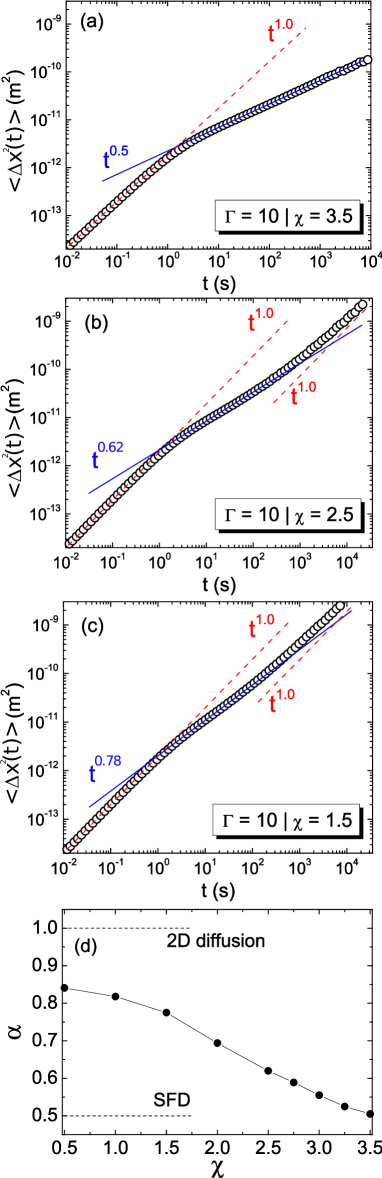
Figure 1: (Color online) (a)-(c) Log-log plot of the mean-square displacement (MSD) $\langle\Delta x^{2}(t)\rangle$ as a function of time for different values of $\chi$. Different diffusion regimes can be distinguished: normal diffusion regime ($\alpha=1.0$) and intermediate subdiffusive regime (ITR, $\alpha<1.0$). Note that for the case of $\chi$ = 1.5, there is a normal diffusion regime (i.e. $\alpha=1.0$) after the ITR. The dashed and solid lines in (a)-(c) are a guide to the eye. Panel (d) shows the dependence of the slope ($\alpha$) of the MSD curves (in the ITR, characterized by an apparent power-law; $\langle\Delta x^{2}(t)\rangle$ $\propto t^{\alpha}$) on the confinement strength $\chi$.

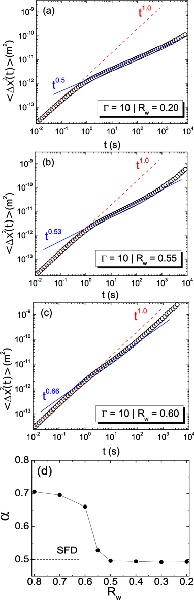
Figure 2: (Color online) (a)-(c) Log-log plot of the mean-square displacement (MSD) $\langle\Delta x^{2}(t)\rangle$ as a function of time for different values of $R_{w}$. Different diffusion regimes can be distinguished: normal diffusion regime ($\alpha=1.0$) and intermediate subdiffusive regime (ITR, $\alpha<1.0$). Note that for the case of $R_{w}$ = 0.60, there is a normal diffusion regime (i.e. $\alpha=1.0$) after the ITR. The dashed and solid lines in (a)-(c) are a guide to the eye. Panel (d) shows the dependence of the slope ($\alpha$) of the MSD curves (in the ITR, characterized by an apparent power-law; $\langle\Delta x^{2}(t)\rangle$ $\propto t^{\alpha}$) on the confinement parameter $R_{w}$.

Initially, in both cases (i.e., a parabolic and a hard-wall confinement potential), the system exhibits a short-time normal diffusion behavior, where $\langle\Delta x^{2}(t)\rangle$ $\propto t^{1.0}$. This is the typical initial “free-particle” diffusion regime. After this initial regime, there is an intermediate subdiffusive regime (ITR). As discussed in Ref. RKutner , the ITR shows an apparent power-law behavior powerlaw , where $0.5<\alpha<1.0$, and it was also found previously in different diffusion models PRB_28_5711 ; AlderAlley . In the ITR, we found a SFD regime for either a channel with strong parabolic confinement [$\chi=3.5$ (Fig. 1(a))] or a narrow hard-wall channel [$R_{w}=0.20$ (Fig. 2(a))]. This is due to the fact that for large (small) values of $\chi$ ($R_{w}$), the confinement prevents particles from passing each other. The results for $\alpha$ in the ITR are shown as a function of $\chi$ and $R_{w}$ in Fig. 1(d) and Fig. 2(d), respectively. As can be seen in Fig. 1(d) [Fig. 2(d)], $\alpha$ increases with decreasing $\chi$ [with increasing $R_{w}$] and thus the SFD condition turns out to be broken. The values of $\alpha$ presented in these figures correspond to the minimum of the effective time dependent exponent $\alpha(t)$. Following Ref. prePZia , $\alpha(t)$ is calculated using the “double logarithmic time derivative”

$$\alpha(t)=\frac{d\,\log\,\langle\Delta x^{2}(t)\rangle}{d\,\log\,t},$$ (15)

and the results are shown in Fig. 3.

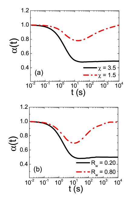
Figure 3: (Color online) (a)-(b) Exponent $\alpha$ as a function of time, calculated from Eq. (15) for different values of the confinement parameters $\chi$ and $R_{w}$, respectively.

The different diffusive regimes, i.e. normal diffusion regime ($\alpha=1.0$) and SFD ($\alpha=0.5$), were also found recently in finite-size systems SJNew ; PMCentres although the transition from SFD to normal diffusion was not analyzed. The $\alpha$-dependence on both the confinement parameters (i.e., $\alpha(\chi)$ and $\alpha(R_{w})$) presents a different qualitative behavior, namely, the SFD regime is reached after a smoother crossover in the parabolic confinement case as compared to the hardwall case. A similar smoother crossover is also found in the case of a circular channel with parabolic confinement in the radial direction. A more detailed discussion on these two different types of the behavior of $\alpha$ will be provided in Sec. IV.

III.2 “Long-time” behavior of the MSD curves and crossing events $C(t)$

For small values of the parabolic confinement (e.g., $\chi=1.5$), the MSD curves present three different diffusive regimes: (i) a short-time normal diffusion regime, where MSD $\langle\Delta x^{2}(t)\rangle$ $\propto t^{1.0}$; (ii) a subdiffusive regime with $\langle\Delta x^{2}(t)\rangle$ $\propto t^{\alpha}$, where $0.5<\alpha<1.0$ and (iii) a “long-time” diffusion regime, which is characterized by $\langle\Delta x^{2}(t)\rangle$ $\propto t^{1.0}$. Note that the “long-time” term used here is not to be confused with the long-time used for infinite systems, as discussed in the Introduction. However, for large values of the parabolic confinement (e.g., $\chi=3.5$), we observe only two distinct diffusive regimes, namely: (i) a short-time normal diffusion regime ($\langle\Delta x^{2}(t)\rangle$ $\propto t^{1.0}$) and (ii) a SFD regime (i.e., $\langle\Delta x^{2}(t)\rangle$ $\propto t^{0.5}$).

One question that arises naturally is whether this normal diffusion regime (i.e., $\langle\Delta x^{2}(t)\rangle$ $\propto t^{1.0}$ for “long-times”) is an effect of the colletive motion of the system (center-of-mass motion) or an effect of the single-particle jumping process, since the confinement potential $\chi=1.5$ allows particles bypass. In order to answer this question, we calculate the number of crossing events $C(t)$ as a function of time and results are shown in Fig. 4(a). We found that for small values of the confinement potential (e.g., $\chi=1.5$) the number of crossing events grows linearly in time, i.e., $C(t)\propto\omega_{c}t$, where $\omega_{c}$ is the rate of crossing events. On the other hand, a strong confinement potential (e.g., $\chi=3.5$) prevents particles from bypassing, and thus $C(t)=0$ during the whole simulation time.

Therefore, the “long-time” normal diffusive behavior (i.e., $\langle\Delta x^{2}(t)\rangle$ $\propto t^{1.0}$ for “long-times”) found in our simulations for the case where the SF (single-file) condition is broken (e.g., $\chi=1.5$) is not due to a collective (center-of-mass) diffusion. Instead, this normal diffusive behaviour is due to a single-particle jumping process, which happens with a constant rate $\omega_{c}>0$ for the case of small values of the confinement ($\chi=1.5$) and $\omega_{c}=0$ (for $\chi=3.5$). The same analysis was done for the case of the hard-wall confinement potential, and the results are found to be the same as for the parabolic confinement.

Nevertheless, we point out that the collective diffusion does indeed exist, but our results from simulations do not allow us to observe this collective (center-of-mass) diffusion regime because of the large size of our chain of particles ($N=400-900$). Simulations with $N=80-100$, and excluding the possibility of mutual bypass (strong confinement potential), allowed us to observe that the $\langle\Delta x^{2}(t)\rangle$ $\propto t^{1.0}$ regime is recovered in the “long-time” limit. In Sec. V, we will further discuss the long-time limit using a model of discrete sites.

As we demonstrated above, the transition from pure 1D diffusion (SFD) characterized by $\alpha=0.5$ to a quasi-1D behavior (with $\alpha>0.5$) could be either more “smooth” (as in Fig. 1(d), for a parabolic confinement) or more “abrupt” (as in Fig. 2(d), for a hard-wall confinement). One can intuitively expect that this difference in behavior can manifest itself also in the crossing events rate $\omega_{c}$, i.e., that $\omega_{c}$ as a function of $\chi$ (or $R_{w}$) should display a clear signature of either “smooth” or “abrupt” behavior.

However, the link between the two quantities, i.e., the exponent, $\alpha(\chi/R_{w})$, and the crossing events rate, $\omega_{c}(\chi/R_{w})$ is not that straightforward. To understand this, let us refer to the long-time limit (which will be addressed in detail within the discrete-site model in Sec. V). As we show, in the long-time limit the exponent $\alpha$ is defined by one of the two conditions: $\omega_{c}=0$ (then $\alpha=0.5$) or $\omega_{c}>0$ (then $\alpha=1$) and it does not depend on the specific value of $\omega_{c}$ provided it is nonzero. Therefore, in the long-time limit the transition between 1D to 2D behavior is not sensitive to the particular behavior of the function $\omega_{c}(\chi/R_{w})$.

Although for “intermediate” times (considered in this section) the condition $\omega_{c}=0$ or $\omega_{c}>0$ is not critical, nevertheless, very small change in the crossing events rate $\omega_{c}(\chi/R_{w})$ strongly influences the behavior of the exponent $\alpha(\chi/R_{w})$. This is illustrated in Figs. 4(b, c). In Fig. 4(b), the function $\omega_{c}(\chi)$ gradually decreases from 1.45 to 0 for $\chi$ varying in a broad interval from 1.5 to 3 (note that the segment of $\omega_{c}(\chi)$ for $2.5<\chi<3$ is nonzero which can be seen in the inset of Fig. 4(b) showing the derivative $d\omega_{c}(\chi)/d\chi$). Correspondingly, the transition from $\alpha=0.5$ to $\alpha\approx 0.8$ in that interval of $\chi$ is “smooth” (see Fig. 1(d)). On the other hand, the function $\omega_{c}(R_{w})$ shown in Fig. 4(c) mainly changes (note the change of the slope $d\omega_{c}(R_{w})/dR_{w}$ shown in the inset of Fig. 4(c)) in a narrow interval $0.5<R_{w}<0.6$. Respectively, the transition for the function $\alpha(R_{w})$ occurs in the narrow interval $0.5<R_{w}<0.6$ and thus is (more) “abrupt”.

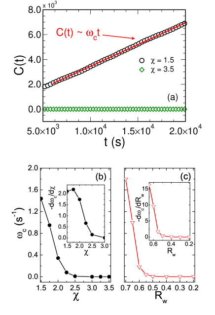
Figure 4: (Color online) (a) Number of crossing events $C(t)$ as a function of time for $N=400$ particles, for $\chi=1.5$ (black open circles) and $\chi=3.5$ (green open diamonds). The solid red line is a linear fit to $C(t)$. Panels (b) and (c) show the rate of the crossing events $\omega_{c}$ as a function of the confinement potential parameters ($\chi$ and $R_{w}$). The insets in the panels (b) and (c) show the derivatives, $d\omega_{c}(\chi)/d\chi$ and $d\omega_{c}(R_{w})/dR_{w}$, correspondingly.

III.3 Distribution of particles along the $y$-direction

For the ideal 1D case, particles are located on a straight line. Increasing the width $R_{w}$ of the confining channel will lead to a zig-zag transition gioPRE ; gioPRB . This zig-zag configuration can be seen as a distorted triangular configuration in this transition zone. Further increase of $R_{w}$ brings the system into the 2D regime, where the normal diffusion behavior is recovered (see Fig. 5).

For the parabolic 1D confinement, we can see [Fig. 6(a)] that the distribution of particles $P(y)$ along the channel is symmetric along the axis $y=0$. Also, for large values of $\chi$ (e.g., $\chi=3.5$) particles are confined in the $y$-direction and thus can move only in the $x$-direction, forming a single-chain structure. As the confinement decreases ($\chi\rightarrow 0$), the distribution of particles $P(y)$ broadens resulting in the crossover from the SFD regime ($\chi=3.5$) to the 2D normal diffusion regime ($\chi=0.5$). Note that for small values of $\chi$ (e.g., $\chi=0.5$), the system forms a two-chain structure (represented by two small peaks of $P(y)$ in Fig. 6(a)), thus allowing particles to pass each other.

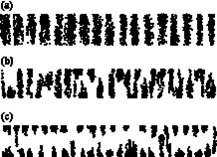
Figure 5: For the hard-wall confinement case, we show typical trajectories of particles (i.e. 10⁶ MD simulation steps) confined by the channel of width (a) $R_{w}=0.20$, (b) $R_{w}=0.60$ and (c) $R_{w}=0.80$.

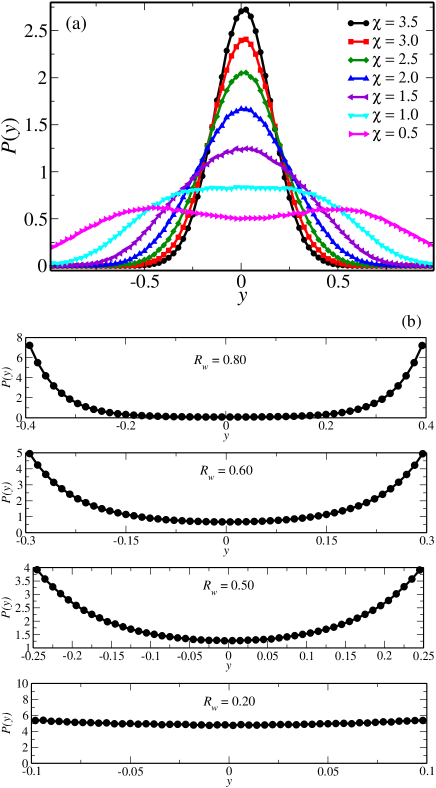
Figure 6: (Color online) Probability distribution of the particle density $P(y)$ along the $y$-direction are shown for (a) different values of $\chi$ (parabolic 1D confinement) and (b) four different values of the width $R_{w}$ of the channel (hard-wall confinement).

IV Diffusion in a circular channel

In the previous section, we analyzed the transition (crossover) from the SFD regime to 2D diffusion in narrow channels of increasing width. The analysis was performed for a straight channel with either hard-wall or parabolic confinement potential. However, in terms of possible experimental verification of the studied effect, one faces an obvious limitation of this model: although easy in simulation, it is hard to experimentally fulfill the periodic boundary conditions at the ends of an open channel. Therefore, in order to avoid this difficulty, in SFD experiments weiScience ; MSJ circular channels were used.

In this section, we investigate the transition (crossover) from SFD to 2D-diffusion in a system of interacting particles diffusing in a channel of circular shape. In particular, we will study the influence of the strength of the confinement (i.e., the depth of the potential profile across the channel) on the diffusive behavior. Without loss of generality, we will adhere to the specific conditions and parameters of the experimental set-up used in Ref. MSJ . An additional advantage of this model is that the motion of the system of charged metallic balls MSJ is not overdamped, and we will solve the full Langevin equations of motion to study the diffusive behavior of the system.

We consider $N$ particles, interacting through a Yukawa potential [Eq. (6)], which are embedded in a ring channel of radius $r_{ch}$. We define a parabolic confinement potential across the channel in the form (5) where parameter $\beta$ is chosen as follows:

$$\beta=\frac{V_{0}}{\gamma r_{0}^{2}},\ \ V_{0}=\frac{q^{2}}{\epsilon}\sum_{i\neq j}\frac{\exp\left[-2\kappa r_{ch}\sin\left(\frac{\phi_{i}-\phi_{j}}{2}\right)\right]}{2r_{ch}\sin\left(\frac{\phi_{i}-\phi_{j}}{2}\right)},$$ (16)

when all the particles are equidistantly distributed along the bottom of the circular channel. It should be noted that in this case, $V_{0}$ is approximately equal to $V_{gs}$ due to the weak Yukawa interaction, which slightly shifts the particles away from the bottom of the channel. Such a choice of $V_{0}$ is related to the fact that we study the influence of the confinement on the diffusion and, therefore, the potential energy of the particles must be of the order of the inter-particle interaction energy. Parameter $r_{0}$ characterizes the distance where the external potential reaches the value $V_{0}/\gamma$, and $V_{gs}$ is the energy of the ground state of the system of $N$ particles as defined by Eq. (7). Parameter $\gamma$ plays the role of a control parameter. By changing $\gamma$ we can manipulate the strength of the confinement and, therefore, control the fulfillment of the single-file condition. Increase in $\gamma$ corresponds to a decrease in the depth of the confinement (5) which leads to the expansion of the area of radial localization of particles. Therefore, an increase of $\gamma$ results in a similar effect (i.e., spatial delocalization of particles) as an increase of temperature, i.e., parameter $\gamma$ can be considered as an “effective temperature”. Note that such a choice of the parameter that controls the confinement strength is rather realistic. In the experiment of Ref. MSJ with metallic balls, the parabolic confinement was created by an external electric field, and the depth of the potential was controlled by tuning the strength of the field.

To study diffusion of charged metallic balls, we solve the Langevin equation of motion in the general form (i.e., with the inertial term $\propto m$),

$$m\frac{d^{2}\vec{r}_{i}}{dt^{2}} = -\eta\frac{d\vec{r}_{i}}{dt}-\sum_{j,i\neq j}\vec{\nabla}V_{int}(\vec{r}_{ij})$$ (17)

$$- \vec{\nabla}V_{c}(\vec{r}_{i})+\vec{F}^{i}_{T},$$

where $m=2.5\times 10^{-6}$ kg MSJ is the mass of a particle, $\eta$ is the friction coefficient (inverse to the mobility). Here all the parameters of the system were chosen following the experiment MSJ , and $\lambda_{D}=4.8\times 10^{-4}~{}m$, $\Gamma=1$ (which is a typical experimental value, see, e.g., also weiScience ). Correspondingly, mass is measured in kg, length in m, and time in seconds. Also, following Ref. MSJ , we took a channel of radius $r_{ch}=9$ mm (in the experiment MSJ , the external radius of the channel was 10 mm, and the channel width 2 mm; note that in our model we do not define the channel width: the motion of a particle in the transverse direction is only restricted by the parabolic confinement potential). We also took experimentally relevant number of diffusing particles, $N$, varying from $N=12$ to $N=40$ (in the experiment MSJ , the ring channel contained $N=12$ or $N=16$ diffusing balls).

Fig. 7 shows the results of calculations of the trajectories of $N=20$ particles diffusing in a ring of radius $r_{ch}=9$ mm for the first 10⁶ MD steps for various values of the parameter $\gamma$. As can be seen from the presented snapshots, the radial localization of particles weakens with increasing $\gamma$. At a certain value of $\gamma$ this leads to the breakdown of the single-file behavior (Figs. 7(c)-(f)).

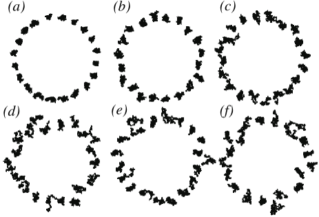
Figure 7: Trajectories of $N=20$ particles diffusing in a ring of radius $r_{ch}=9$ mm for $10^{6}$ consequent time steps for different values of $\gamma$. $\gamma$=1 (a), 2 (b), 3 (c), 5 (d), 7 (e), 9 (f).

IV.1 Breakdown of SFD

It is convenient to introduce the distribution of the probability density of particles in the channel $P_{\text{rad}}$ along the radial direction $r$. In order to calculate the function $P_{\text{rad}}(r)$ we divided the circular channel in a number of coaxial thin rings. The ratio of the number of observations of particles in a sector of radius $r_{i}$ to the total number of observations during the simulation is defined as the probability density $P_{\text{rad}}(r_{i})$. In Fig. 8, the probability density $P_{\text{rad}}(r)$ is presented for different values of $\gamma$. With increasing $\gamma$, the distribution of the probability density $P_{\text{rad}}(r)$ broaden and the maximum of the function $P_{\text{rad}}(r)$ shifts away from the center of the channel (see Fig. 8). The latter is explained by the softening of the localization of particles with increasing $\gamma$, which tend to occupy an area with a larger radius due to the repulsive inter-particle interaction. Simultaneously, the distribution of the probability density $P_{\text{rad}}(r)$ acquires an additional bump indicating the nucleation of a two-channel particle distribution nonzigzag . The observed broadening and deformation of the function $P_{\text{rad}}(r)$ is indicative of a gradual increase of the probability of mutual bypass of particles (i.e., the violation of the SF (single-file) condition, also called the “overtake probability” ambjornsson ) with increasing $\gamma$.

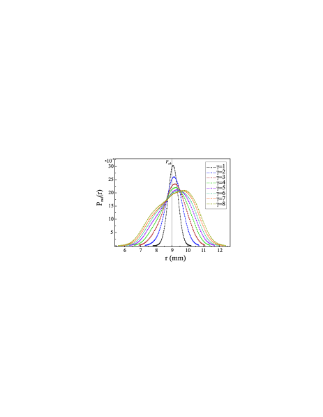
Figure 8: (Color online) The distribution of the probability density of particles $P_{\text{rad}}(r)$ in a circular channel of radius $r_{ch}=9$ mm along the radial direction $r$. The different curves correspond to various $\gamma$. Increasing $\gamma$ the width of the distribution $P_{\text{rad}}(r)$ increases due to a weakening of the confinement.

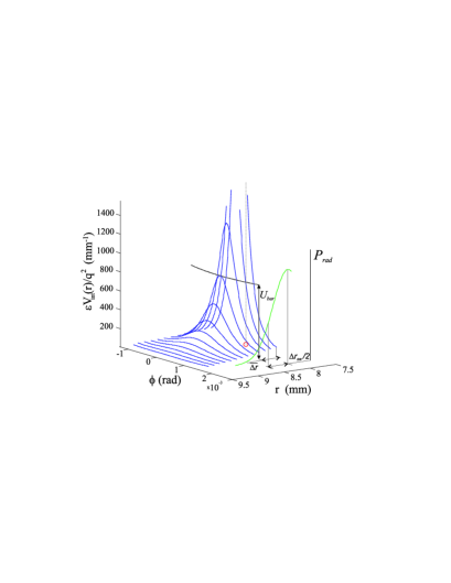
Figure 9: (Color online) Spatial distribution of the potential $V_{int}(r,\phi)$ created by a particle (red (grey) circle) and the qualitative distribution of the probability density of particles in circular channel $P_{\text{rad}}(r)$ (green (light grey) line) along the radial direction $r$. The function $\overline{\Delta r}$ determines an approximate radial distance between particles when the potential barrier $U_{bar}$ becomes “permeable” for given temperature $T$. The function $\Delta r_{sw}$ characterizes a width of the distribution $P_{\text{rad}}(r)$ at this temperature $T$.

Let us now discuss a qualitative criterion for the breakdown of SFD, i.e., when the majority of particles leave the SFD mode. For this purpose, let us consider a particle in the potential created by its close neighbor (which is justified in case of short-range Yukawa interparticle interaction and low density of particles in a channel) shown in Fig. 9. Different lines show the interparticle potential $V_{int}$ as a function of angle $\phi$ for different radii $r$. For small values of $\gamma$, the center of the distribution $P_{\text{rad}}(r)$ (see Fig. 7) almost coincides with the center of the channel (i.e., with the minimum of the confinement potential profile) and the distribution $P_{\text{rad}}(r)$ is narrow. Therefore, mutual passage of particles is impossible, i.e., the SF condition is fulfilled. The asymmetric broadening of the function $P_{\text{rad}}(r)$ with increasing $\gamma$ results in an increasing probability of mutual bypass of particles which have to overcome a barrier $U_{bar}$ (see Fig. 9). This becomes possible when $U_{bar}\lesssim k_{B}T$. In other words, the thermal energy $k_{B}T$ determines some minimal width $\overline{\Delta r}$ between adjacent particles when the breakdown of the SF condition becomes possible.

It is clear that “massive” violation of the SF condition (i.e., when the majority of particles bypass each other) occurs when the halfwidth $\Delta r_{sw}$ of the distribution of the probability density $P_{\text{rad}}(r)$ obeys the condition:

$$\Delta r_{sw}\gtrsim\overline{\Delta r}.$$ (18)

The function $\Delta r_{sw}$ is defined by the ratio of the thermal energy $k_{B}T$ to the external potential $U_{conf}(r)$ and is of the same order as $\widetilde{\Delta r}$:

$$\frac{V_{0}}{\gamma r_{0}^{2}}\cdot(\widetilde{\Delta r}/2)^{2}\approx k_{B}T.$$ (19)

Therefore the criterion (18) can be presented in the form:

$$\Delta r_{sw}\approx\widetilde{\Delta r}\gtrsim\overline{\Delta r}.$$ (20)

This qualitative analysis of the breakdown of the SFD regime clarifies the role of the width and the shape of the distribution of the probability density influenced by the asymmetry of the circular channel.

IV.2 Diffusion regimes

The MSD $\langle\Delta\phi^{2}(t)\rangle$ is calculated as a function of time $t$ as:

$$\left\langle\Delta\phi^{2}(t)\right\rangle=\left\langle\frac{1}{N_{\text{par}}N_{\text{ens}}}\sum_{i,j}\left[\Delta\phi_{ij}(\tau+t)-\Delta\phi_{ij}(t)\right]^{2}\right\rangle_{t},$$ (21)

where $N_{\text{par}}$ is the total number of particles of an ensemble and $N_{\text{ens}}$ is the total number of ensembles. In our calculations, the number of ensembles was chosen 100 for a system consisting of 20 particles.

The time dependence of the MSD for different values of $\gamma$ is shown in Fig. 10(a)–(c). Initially the system exhibits normal diffusion, where $\langle\Delta\phi^{2}\rangle$ $\propto t^{1.0}$. This regime is followed by an intermediate subdiffusive regime, where the $\langle\Delta\phi^{2}\rangle$ $\propto t^{\alpha}$ ($0.5<\alpha<1.0$). For longer times, the system recovers “long-time” normal diffusion (see discussions in Sec. IIIB), with $\langle\Delta\phi^{2}\rangle$ $\propto t^{1.0}$. As in the case of straight channel geometry, this second crossover (i.e., from intermediate subdiffusion to “long-time” normal diffusion) can also be due to two other reasons: (i) due to a collective (center-of-mass) diffusion or (ii) due to a single-particle jumping process. However, for the simulations in the case of a circular geometry, the number of particles is relatively small (taking the fact that this is a finite-size system), and therefore, the crossover from sublinear to linear regime is due to a collective (center-of-mass) diffusion. We further address this issue in Sec. V, where we consider a discrete site model and we exclude the center-of-mass motion.

Fig. 10(d) shows $\alpha$ as a function of $\gamma$. The function $\alpha(\gamma)$ experiences a monotonic gradual crossover from the $\alpha=0.5$ to a $\alpha\lesssim 1$-regime. Note that the observed deviation from the normal diffusion behavior for large $\gamma$ (Fig. 10) is related to the presence of, though weak but nonzero, external confinement in the radial direction. This change of the diffusive behavior is explained by a weakening of the average radial localization of particles with increase of $\gamma$ (Fig. 8) and, as a consequence, by an increase of the probability of mutual bypass of particles.

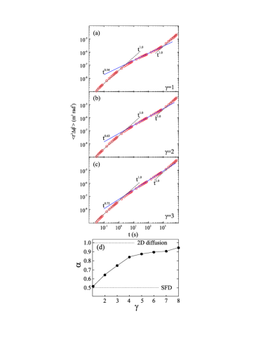
Figure 10: (Color online) (a)–(c): Log-log plot of the mean-squared displacement (MSD) $\langle\Delta\phi^{2}\rangle$ as a function of time for different values of the “effective” temperature $\gamma$ = (a) 1, (b) 2, and (c) 3. Here $(N_{\text{ens}}=100,N_{\text{par}}=20)$. (d) The diffusion exponent $\alpha$ as a function of $\gamma$. Increase of the “effective” temperature $\gamma$ leads to the gradual transformation of the single-file regime of diffusion into the diffusion regime of free particles.

The observed crossover between the 1D single-file and 2D diffusive regimes, i.e., $\alpha(\gamma)$-dependence, shows a significant different qualitative behavior as compared to the case of a hard-wall confinement potential considered in Sec. III, where a rather sharp transition between the two regimes was found [Fig. 2(d)]. The different behavior is due to the different confinement profiles and can be understood from the analysis of the distribution of the probability density of particles for these two cases. In the case of a hard-wall channel, the uncompensated (i.e., by the confinement) interparticle repulsion leads to a higher particle density near the boundaries rather than near the center of the channel (see Fig. 5 and Fig. 6(b)). As a consequence, the breakdown of the SF condition — with increasing width of the channel — happens simultaneously for many particles in the vicinity of the boundary resulting in a sharp transition (see Fig. 2(d)). On the contrary, in the case of parabolic confinement, the density distribution function has a maximum — sharp or broad, depending on the confinement strength — near the center of the channel (see Figs. 6(a) and 8). With increasing the “width” of the channel (i.e., weakening its strength), only a small fraction of particles undergoes the breakdown of the SF condition. This fraction gradually increases with decreasing strength of the confinement, therefore resulting in a smooth crossover between the two diffusion regimes.

V Discrete site model: The long-time limit

The calculated MSD for different geometries and confinement potentials allowed us to explain the evolution of the subdiffusive regime with varying width of the channel (or potential strength in case of a parabolic potential). However, the obtained results are only valid for the intermediate regime and therefore they only describe the “onset” of the long-time behavior. The problem of accessing the long-time behavior in a finite chain is related to the fact that sooner or later (i.e., depending on the chain length) the interacting system will evolve into a collective, or “single-particle”, diffusion mode which is characterized by $\alpha=1.0$. Thus the question is whether the observed behavior holds for the long-time limit, i.e., is the transition from $t^{0.5}$ to $t^{1.0}$ behavior smooth?

To answer this question, we considered a simple model, i.e., a linear discrete chain of fixed sites filled with either particles or “holes” (i.e., sites not occupied by particles) (for details, see Ref. PRB_28_5711 ; this model was also recently used in Ref. SSPRE2006 ). The particles can move along the chain only due to the exchange with adjacent vacancies (i.e., with holes). Within this model, the long-time diffusion behavior was described analytically for an infinite linear chain as well as for a finite cyclic chain PRB_28_5711 . In particular, this model predicts that: (i) If the chain is infinite then the long-time power law of the diffusion curve $\alpha$ is $0.5$ (i.e., MSD $\langle\Delta x^{2}(t)\rangle$ $\propto t^{0.5}$); (ii) If the chain is finite then the subdiffusive regime with $\alpha=0.5$ is followed by either $\alpha=1.0$ regime (if the cyclic boundary condition is realized), or by $\alpha=0$ regime, i.e., the regime of saturation (if no cyclic boundary condition is imposed PRE80-051103 ). The latter regime is reached for times longer than the “diffusion time” of a “hole” along the whole chain $t_{\text{chain}}$.

Let us now apply this model to a finite-size chain of particles. For this purpose, we assume that adjacent particles are able to exchange their positions with some probability $P$ at every time step. For example, probability $P=0.1$ means that a couple of any adjacent particles certainly exchange their positions once for every $10$ time steps.

The results of our calculations of the MSD performed using this model are presented in Fig. 11(a). We used the following parameters: the chain length is $N_{s}=150$ sites and $N_{h}=1$ hole. Averaging was done over $1000$ ensembles. The calculation was performed for the following values of the probability: $P=0,10^{-5},10^{-4},10^{-3},0.01,0.1$, and $1$.

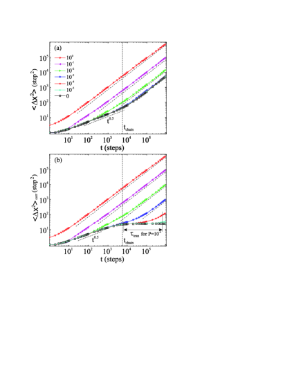
Figure 11: (Color online) Log-log plot of the MSD $\langle\Delta x^{2}(t)\rangle$ (a) and corrected MSD $\langle\Delta x^{2}(t)\rangle$${}_{\text{corr}}$ (b) as a function of time for different values of the probability $P$ of bypassing. Averaging was done over $N_{\text{sim}}=1000$ ensembles.

We see in Fig. 11(a) clearly the above-mentioned two diffusion regimes, i.e., with the MSD $\langle\Delta x^{2}(t)\rangle$ $\propto t^{0.5}$ and $\propto t^{1.0}$. The characteristic time $t_{\text{chain}}$ shifts towards lower values with increasing $P$. However this analysis (Fig. 11(a)) does not allow to distinguish the contributions to the long-time behavior ($\propto t^{1.0}$) due to: (i) the breakdown of single-file condition (i.e., diffusion due to particle exchanges), and (ii) the “collective” diffusion (chain “rotation”).

To overcome this difficulty, we exclude the “collective” diffusion of the system and introduce a modified MSD $\langle\Delta x^{2}(t)\rangle$${}_{\text{corr}}$ (which is so-called “roughness” of the system of particles, as discussed in Ref. PMCentres ) as follows:

$$\langle\Delta x^{2}\rangle_{\text{corr}}=\langle(x-\bar{x})^{2}\rangle,$$

where $\langle...\rangle$ is the average over time; $\bar{x}$ is the average of an ensemble of particles at a given time, or “collective” coordinate. It should be noted that $\langle x\rangle\neq\bar{x}$. If the system does not experience “collective” diffusion then $\bar{x}(t)=0$ and the modified MSD coincides with the conventional one:

$$\langle\Delta x^{2}\rangle_{\text{corr}}=\langle x^{2}\rangle.$$

The diffusion curves calculated by using the modified MSD are presented in Fig. 11(b). For $P=0$, the diffusion curve (shown by black open squares) after the subdiffusive regime reaches saturation (i.e., $\langle\Delta x^{2}(t)\rangle$${}_{\text{corr}}$ = const). The observed behavior is similar to that of a finite linear chain with fixed ends (see Ref. PRE80-051103 ). For $P\neq 0$, all the diffusion curves in the long-time limit are characterized by $\alpha=1.0$, independent of the value of the probability $P$, as seen in Fig. 11(b). In other words, the long-time diffusion does not depends on the probability of mutual exchanges of particles and has the same long-time behavior for any probability $P\neq 0$. Here we would like to emphasize again that the long-time behavior of the diffusion curves is free from the “collective” diffusion effect and is only determined by particle jump diffusion. Increasing a number of sites in the model corresponds, in fact, approaching to the model of infinite chain. We have found that the increasing a number of sites leads to growth of the $\langle\Delta x^{2}(t)\rangle$${}_{\text{corr}}$ limit of saturation, on the one hand, and to a shift of $t_{\text{chain}}$ to larger $t$, on the other hand. Hence, extrapolating our results to the case of infinite chain, we can conclude that in this case as well as in the case of finite-size chain, the breakdown of single-file condition leads to an abrupt transition from subdiffusive to the normal diffusion regime.

The difference in the diffusive curves is just the time $\tau_{\text{tran}}$ from subdiffusive regime to the normal regime: for low $P$ it ($\tau_{\text{tran}}$) is long enough while for high $P$ it ($\tau_{\text{tran}}$) is short. It is easy to see that $\tau_{\text{tran}}\sim 1/P(\%)$. Thus, we can conclude that in the long-time limit the transition from $~{}t^{0.5}$ to $~{}t^{1.0}$ behavior is abrupt. Note that our calculations performed using the modified MSD $\langle\Delta x^{2}(t)\rangle$${}_{\text{corr}}$ reproduce the results of Ref. PRE80-051103 for a closed “box”. This is explained by the fact that in the closed “box” geometry the center of mass (or collective) diffusion is zero, and it is natural that the roughness (see Ref. PMCentres ) and the particles diffusion coincide.

VI Conclusions

We have studied a monodisperse system of interacting particles subject to three types of confinement potentials: (i) a 1D hardwall potential, (ii) a 1D parabolic confinement potential which both characterize a quasi-1D system, and (iii) a circular confining potential, which models a finite size system. In order to study the diffusive properties of the system, we have calculated the mean-squared displacement (MSD) numerically through molecular dynamics (MD) simulations. For the case where particles diffuse in a straight line in a Q1D channel, different diffusion regimes were found for different values of the parameters of the confining potential ($\chi$ or $R_{w}$). We have found that the normal diffusion is suppressed if the channel width $R_{w}$ is between $0.20$ and $0.50$ (or by $2.0<\chi<3.5$, for the case of parabolic 1D confinement), leading the system to a SFD regime for intermediate time scales. For values of $R_{w}\geqslant 0.56$, particles will be able to cross each other and the SFD regime will be no longer present.

The case of a circular channel corresponds to, e.g., the set-up used in experiments with sub-millimetric metallic massive balls diffusing in a ring with a parabolic potential profile created by an external electric field. The strength of the potential (which determines the effective “width” of the channel) can be tuned by the field strength. Contrary to the case of hard-wall confinement, where the transition (regarding the calculation of the scaling exponent ($\alpha$) of the MSD $\langle\Delta x^{2}(t)\rangle$$\propto t^{\alpha}$) is sharp, a smooth crossover between the 1D single-file and the 2D diffusive regimes was observed. This behavior is explained by different profiles for the distribution of the particle density for the hard-wall and parabolic confinement profiles. In the former case, the particle density reaches its maximum near the boundaries of the channel resulting in a massive breakdown of the SF condition and thus in a sharp transition between the different diffusive regimes. In the latter case, on the contrary, the density distribution function has a maximum near the center which broadens with decreasing strength of the confinement. This results in a smooth crossover between the two diffusion regimes, i.e., SFD and 2D regime. The analysis of the crossing events, i.e., the rate of the crossing events $\omega_{c}$ as a function of the confinement parameter $\chi$ or $R_{w}$, supports these results: the function $\omega_{c}(\chi/R_{w})$ displays a clear signature of either “smooth” or “abrupt” behavior.

We also addressed the case of a finite discrete chain of diffusing particles. It was shown that in this case the breakdown of the single-file condition (i.e., when the probability $P$ of particles bypassing each other is non-zero) leads to an abrupt transition from a subdiffusive regime to the normal diffusion regime.

References

- (1) C. Cottin-Bizonne, J.-L. Barrat, L. Bocquet, and E. Charlaix, Nature Mater. 2 237 (2003).
- (2) L. A. Hodgkin and D. R. Keynes, J. Physiol. 128, 61 (1955).
- (3) Jörg Kärger, Phys. Rev. A 45, 4173 (1992).
- (4) F. Martin, R. Walczak, A. Boiarski, M. Cohen, T. West, C. Cosentino, J. Shapiro, and M. Ferrari, J. Control. Release 102, 123 (2005).
- (5) T. E. Harris, J. Appl. Probab. 2, 323 (1965).
- (6) P. Barrozo, A. A. Moreira, J. A. Aguiar, and J. S. Andrade Jr., Phys. Rev. B 80, 104513 (2009).
- (7) J. S. Andrade, Jr., G. F. T. da Silva, A. A. Moreira, F. D. Nobre, and E. M. F. Curado, Phys. Rev. Lett. 105, 260601 (2010).
- (8) G. Hummer, J. C. Rasaiah, and J. P. Noworyta, Nature (London) 414, 188 (2001).
- (9) M. W. Meier and H. D. Olsen (Editors), Atlas of Zeolite Structure Types (Butterworths-Heinemann, London 1992).
- (10) T. Halpin-Healy and Y. C. Zhang, Phys. Rep. 254, 215 (1995).
- (11) L. J. Lebowitz and K. J. Percus, Phys. Rev. E 155, 122 (1967).
- (12) D. G. Levitt, Phys. Rev. A 8, 3050 (1973).
- (13) P. M. Richards, Phys. Rev. B 16, 1393 (1977).
- (14) L. Lizana and T. Ambjörnsson, Phys. Rev. E 80, 051103 (2009).
- (15) V. N. Kharkyanen and Semen O. Yesylevskyy, Phys. Rev. E 80, 031118 (2009).
- (16) E. Barkai and R. Silbey, Phys. Rev. Lett. 102, 050602 (2009).
- (17) A. M. Alsayed, M. F. Islam, J. Zhang, P. J. Collings, and A. D. Yodh, Science 309, 1207 (2005).
- (18) H.-Q. Wei, C. Bechinger, and P. Leiderer, Science 287, 625 (2000).
- (19) C. Lutz, M. Kollmann, and C. Bechinger, Phys. Rev. Lett. 93, 026001 (2004).
- (20) G. Piacente, F. M. Peeters, and J. J. Betouras, Phys. Rev. E 70, 036406 (2004).
- (21) W. P. Ferreira, J. C. N. Carvalho, P. W. S. Oliveira, G. A. Farias, and F. M. Peeters, Phys. Rev. B 77, 014112 (2008).
- (22) W. Yang, K. Nelissen, M. Kong, Z. Zeng, and F. M. Peeters, Phys. Rev. E 79, 041406 (2009).
- (23) K. Nelissen, V. R. Misko, and F. M. Peeters, Europhys. Lett. 80, 56004 (2007).
- (24) For underdamped systems, the initial fast growth of the MSD (i.e., ballistic regime) is characterized by .
- (25) G. Coupier, M. SaintJean, and C. Guthmann, Phys. Rev. E 73, 031112 (2006).
- (26) H. L. Tepper, J. P. Hoogenboom, N. F. A. van der Vegt, and W. J. Briels, J. Chem. Phys. 110, 11511 (1999).
- (27) J. B. Delfau, C. Coste, and M. Saint-Jean, Phys. Rev. E 84, 011101 (2011).
- (28) P. M. Centres and S. Bustingorry, Phys. Rev. E 81, 061101 (2010).
- (29) D. V. Tkachenko, V. R. Misko, and F. M. Peeters, Phys. Rev. E 82, 051102 (2010).
- (30) B. Lin, M. Meron, B. Cui, S. A. Rice, and H. Diamant, Phys. Rev. Lett. 94, 216001 (2005).
- (31) D. L. Ermak and J. A. McCammon, J. Chem. Phys. 69, 1352 (1978).
- (32) As recently shown when studying single-trajectory averages pre85JeonMetzler , time average (TA) may differ from ensemble average (EA) MSD not only for nonergodic processes (for example, for anomalous diffusion described by continuous time random walks (CTRWs) models EBarkaiPRL ; Klafter ), but also for some ergodic processes in small complex systems.
- (33) J-H. Jeon and R. Metzler, Phys. Rev. E 85, 021147 (2012).
- (34) Y. He, S. Burov, R. Metzler, and E. Barkai, Phys. Rev. Lett. 101, 058101 (2008).
- (35) A. Lubelski, I. M. Sokolov, and J. Klafter, Phys. Rev. Lett. 100, 250602 (2008).
- (36) R. Kutner, H. van Beijeren, and K. W. Kehr, Phys. Rev. B 30, 4382 (1984).
- (37) This apparent power-law behavior is characterized by MSD , and it is an intermediate phenomena due to the interplay between the crossover from the MSD regime to regime. For details, see Ref. RKutner .
- (38) H. van Beijeren, K. W. Kehr, and R. Kutner, Phys. Rev. B 28, 5711 (1983).
- (39) B. J. Alder and W. E. Alley, J. Stat. Phys. 19, 341 (1978).
- (40) Y-L. Chou, M. Pleimling, and R. K. P. Zia, Phys. Rev. E 80, 061602 (2009).
- (41) G. Piacente, G. Q. Hai, and F. M. Peeters, Phys. Rev. B 81, 024108 (2010).
- (42) Note that this is not a zig-zag transition: the function still has a single maximum which is shifted from the center of the channel.
- (43) T. Ambjörnsson and R. J. Silbey, J. Chem. Phys. 129, 165103 (2008).
- (44) S. Savel’ev, F. Marchesoni, A. Taloni, and F. Nori, Phys. Rev. E 74, 021119 (2006).